A Non-Cooperative Method for Path Loss Estimation in Femtocell Networks

Abstract

A macrocell superposed by indoor deployed femtocells forms a geography-overlapped and spectrum-shared two-tier network, which can efficiently improve coverage and enhance system capacity. To reduce inter-tier co-channel interference, femtocell user should choose suitable access channel according to the path losses between itself and the macrocell users. Path loss should be estimated non-cooperatively since information exchange is difficult between macrocell and femtocells. In this paper, a novel method is proposed for femtocell user to estimate the path loss between itself and any macrocell user independently. According to the adaptive modulation and coding (AMC) mode information broadcasted by the macrocell base station (BS), femtocell user first estimates the path loss between BS and a macrocell user by using Maximum a Posteriori (MAP) method. The probability density function (PDF) and statistics of the transmission power of the macrocell user are then derived. According to the sequence of received power values from the macrocell user, femtocell user estimates the path loss between itself and the macrocell user by using minimum mean square error (MMSE) method. Simulation results show that the proposed method can efficiently estimate the path loss between any femtocell user and any macrocell user in all kinds of conditions.

I Introduction

The two-tier network formed by deploying femtocells in the coverage of an already existed macrocell can improve indoor coverage and enhance system overall capacity by sharing spectrum between these two tiers [1]. In the view of cognitive radio [2], the macrocell is the primary tier whose users and base station (BS) communicate to each other and have a priority to use channels, the femtocells are of the secondary tier whose users can communicate with their access points (APs) under the premise of no obvious influence on the communication in primary tier network. For the conciseness of presentation, femtocell user is called SU (secondary user), while macrocell user is called PU (primary user) in this article.

The spectrum sharing in this two-tier network leads to not only high spectrum efficiency but also serious inter-tier interference. If SU knows the path losses between itself and all the PUs, then each SU can choose the channel occupied by a PU far away from it so as to reduce the inter-tier co-channel interference. Therefore, the estimation of path loss between SU and PU plays a very important role in femtocell networks.

Existing methods for estimating the path loss between two locations can be classified into two types, that is, model-based method and measurement-based method. In the model-based methods [5], the estimating end calculates the path loss according to the known propagation loss model and distance between the two ends. However, for the SU, which works as the estimating end, it is very difficult to obtain the distances between itself and a PU in a real two-tier network. On the other hand, in the measurement-based methods [6, 7, 8], the estimating end first obtains the transmission power of the other end, and then calculates the path loss as the ratio of the received power to the transmission power. Here, the transmission power value is either fixed and known to the estimating end, such as the pilot signal, or is included in a packet which is transmitted to the estimating end. In the literature, existing measurement-based methods require the estimating end to be informed explicitly of the transmission power of the other end. That is, the two ends should work cooperatively. However, PU’s transmission power depends on its location, channel status, required SINR etc, and inter-tier information exchange should not be assumed in a real two-tier network. Therefore, for an SU (the estimating end), it is very hard to know the value of a PU’s transmission power.

To solve the above problem, this paper proposes a novel path loss estimation method for an SU to independently estimate the path loss between itself and PUs in two-tier network. Similar to the existing measurement-based methods, the proposed method also consists of two steps. Firstly, SU demodulates the BS broadcast information and obtains the downlink and uplink adaptive modulation and coding (AMC) modes used by the transmitting signals of BS and PU. SU estimates the path loss between the PU and BS according to the AMC modes, and derives the probability density function (PDF) and statistics of the PU’s transmission power. Secondly, after measuring the received power from the PU, SU estimates the path loss between itself and the PU by exploiting the relation among transmission power, received power and path loss. This method only utilizes the AMC mode information broadcast by BS and the statics of channel between BS and PU, while does not need any information exchange between SU and PU. This non-cooperative estimation method does not have any impact on the macrocell network.

This paper is organized as follows. The mathematical models of AMC mode assigned by BS for PU transmission signal, PU transmission power and SU received power are established in Section II. In Section III, the PDF and statistics of PU transmission power are derived. The estimation method of path loss between SU and PU is given in Section IV. Simulation results are given in Section V, followed by conclusions in Section VI.

II System model

The considered system model is shown in Fig. 1. The macrocell is a normal cell of a cellular network, in which PU and BS communicate to each other and have priority to use the channels. BS broadcasts information of AMC modes of the transmission signals in the downlink and uplink for demodulation and modulation in the cell. By sharing spectrum with PU, SU can communicate with its access point (AP) under the condition that the macrocell user is not affected obviously.

Figure 1: System structure

II-A AMC mode assigned by BS

In the main stream cellular networks, such as WiMAX and LTE, BS uses a constant transmission power in the downlink for convenience, and assigns an appropriate AMC mode for BS transmission signal according to channel status so as to make the best use of channel capacity. Denote the transmission power of BS as $P_{0}$. Then, the SINR of the received signal of PU at time instant $i$ can be written as

$${S_{d,i}=\frac{{P_{0}\left|{h_{bp,i}}\right|^{2}}}{{\sigma^{2}L_{bp}}},\;\;\;i=1,\;2,\;\cdots,\;I},$$ (1)

where the subscript $d$ represents downlink; $h_{bp,i}$ is the channel response between BS and PU at time instant $i$, whose absolute value obeys the Rayleigh distribution; $\sigma^{2}$ is the average power of background noise; $L_{bp}$ is the downlink path loss between BS and PU; $I$ is the number of observations.

Suppose there are $M$ available AMC modes, where mode sequence number $m=1,2,\cdots,M$. The order of the $(m+1)$-th mode is higher than that of the $m$-th mode, and the required receiving SINR of the $(m+1)$-th mode is also higher. The sequence number of AMC mode assigned by BS for its transmission signal at time instant $i$ can be represented as

$${m_{d,i}=\Psi\left({S_{d,i}}\right),\;\;\;i=1,\;2,\;\cdots,\;I},$$ (2)

where $m_{d,i}\in\{1,2,...M\}$; $\Psi\left(\cdot\right)$ stands for an assignment function, which produces a sequence number of AMC mode which satisfies the required receiving SINR requirement and maximizes the transmission rates. The sequence number of AMC modes assigned by BS for its transmission signals in the last $I$ instants composes a vector ${\bf{m}}_{d}=[m_{d,1},\;\cdots,m_{d,i},\;\cdots,\;m_{d,I}]^{\rm{T}}$.

II-B PU transmission power

In the uplink, PU adjusts its transmission power so that the received SINR of BS satisfies the requirement of adopted AMC mode exactly, as applied in WiMAX and LTE systems. The transmission power of PU at time instant $i$ can be written as

$${P_{t,i}=\left\{\begin{array}[]{l}P_{\min},\;\;\;\;\;\;\;\;\;\;\;\;\tilde{P}_{t,i}<P_{\min}\\ \tilde{P}_{t,i},\;\;\;\;\;P_{\min}\leq\tilde{P}_{t,i}\leq P_{\max}\\ P_{\max},\;\;\;\;\;\;\;\;\;\;\;\;\tilde{P}_{t,i}>P_{\max}\\ \end{array}\right.,\;\;\;\;i=1,\;2,\;\cdots,\;I},$$ (3)

where the subscript $t$ represents transmission; $P_{\min}$ and $P_{\max}$ are the minimum and maximum allowed transmission powers of PU. When no power restriction is imposed, in order to satisfy the required receiving SINR, the PU’s transmission power can be expressed as

$${\tilde{P}_{t,i}=\frac{{\Omega\left({m_{u,i}}\right)L_{pb}}}{{\left|{h_{pb,i}}\right|^{2}}}\sigma^{2}},$$ (4)

where $m_{u,i}$ is the sequence number of the AMC mode assigned by BS for PU’s transmission signal at time instant $i$; subscript $u$ represents uplink; $\Omega\left(m\right)$ stands for a mapping function, which produces the required minimum SINR according to the sequence number of the AMC mode $m$; $L_{pb}$ is the path loss between PU and BS in the uplink; $h_{pb,i}$ is the channel response between PU and BS at time instant $i$.

II-C Received power of SU

When PU transmits signal to BS with power $P_{t,i}$ at time instant $i$, the SU’s received power of the signal transmitted by PU can be expressed as

$${\begin{array}[]{l}P_{r,i}=\frac{{P_{t,i}\left|{h_{ps,i}}\right|^{2}}}{{L_{ps}}}+P_{N,i}\\ \;\;\;\;\;=P_{t,i}\left|{h_{ps,i}}\right|^{2}x+P_{N,i},\;\;\;\;i=1,\;2,\;\cdots,\;I\\ \end{array}},$$ (5)

where subscript $r$ represents receiving; $h_{ps,i}$ is the channel response between PU and SU at time instant $i$; $x$ is the inversion of the path loss between PU and SU; $P_{N,i}$ is the power of background noise at time instant $i$, which is a random variable following the $\chi^{2}$ distribution of one degree of freedom with mean value equal to $\sigma^{2}$ . Equation $(5)$ can be expressed in matrix form as

$${{\bf{P}}_{r}=diag\left({{\bf{P}}_{t}}\right)\cdot{\bf{h}}_{ps}x+{\bf{P}}_{N}},$$ (6)

where ${\bf{P}}_{r}$ is the received power vector, and ${\bf{P}}_{r}=[P_{r,1},\;\cdots,P_{r,i},\;\cdots,\;P_{r,I}]^{\rm{T}}$; ${\bf{P}}_{t}$ is the transmission power vector, and ${\bf{P}}_{t}=[P_{t,1},\;\cdots,P_{t,i},\;\cdots,\;P_{t,I}]^{\rm{T}}$; $diag\left({{\bf{P}}_{t}}\right)$ is a diagonal matrix composed of the elements in vector ${\bf{P}}_{t}$; ${\bf{h}}_{ps}$ is the channel response vector, and ${\bf{h}}_{ps}=[\left|{h_{ps,1}}\right|^{2},\cdots,\;\left|{h_{ps,i}}\right|^{2},\;\cdots,\;\left|{h_{ps,I}}\right|^{2}]^{\rm{T}}$; ${\bf{P}}_{N}$ is the noise power vector, and ${\bf{P}}_{N}=[P_{N,1},\;\cdots,P_{N,i},\;\cdots,\;P_{N,I}]^{\rm{T}}$.

III PDF and statistics of PU transmission power

In order to estimate the path loss between SU and PU, SU needs to know the transmission power of PU. In this section, SU first estimates the path loss between PU and BS by exploiting the information of AMC mode assigned by BS in the downlink and then derives the PDF and statistics of PU transmission power ${\bf{P}}_{t}$.

III-A Estimation of path loss $L_{pb}$ between PU and BS

We first derive the joint PDF of the AMC mode sequence number vector ${\bf{m}}_{d}$ and the path loss $L_{bp}$ and then estimate the path loss $L_{pb}$ by using MAP method.

According to Equations $(1)$ and $(2)$, when $L_{bp}$ is known, the probability that BS assigns the $m_{d,i}$-th AMC mode for its transmission signal at time instant $i$ can be expressed as

$${\begin{array}[]{l}P\left({m_{d,i}|L_{bp}}\right)=P\left({\Omega\left({m_{d,i}}\right)\leq S_{d,i}<\Omega\left({m_{d,i}+1}\right)}\right)\\ \;\;\;\;\;\;\;\;\;\;\;\;\;\;=P\left({\frac{{\Omega\left({m_{d,i}}\right)L_{bp}\sigma^{2}}}{{P_{0}}}\leq\left|{h_{bp,i}}\right|^{2}<\frac{{\Omega\left({m_{d,i}+1}\right)L_{bp}\sigma^{2}}}{{P_{0}}}}\right)\\ \;\;\;\;\;\;\;\;\;\;\;\;\;\;=F_{y}\left({\frac{{\Omega\left({m_{d,i}+1}\right)L_{bp}\sigma^{2}}}{{P_{0}}}}\right)-F_{y}\left({\frac{{\Omega\left({m_{d,i}}\right)L_{bp}\sigma^{2}}}{{P_{0}}}}\right)\\ \;\;\;\;\;\;\;\;\;\;\;\;\;\;=e^{-\;\frac{{\Omega\left({m_{d,i}}\right)L_{bp}\sigma^{2}}}{{P_{0}}}}-e^{-\;\frac{{\Omega\left({m_{d,i}+1}\right)L_{bp}\sigma^{2}}}{{P_{0}}}}\\ \end{array}},$$ (7)

where the third equality is because $\left|{h_{bp,i}}\right|^{2}$ is a random variable following the standard $\chi^{2}$ distribution of two degrees of freedom , whose cumulative distribution function (CDF) is $F_{y}(y)=1-e^{-y}$ [9].

Suppose PU is uniformly distributed in the Macrocell. Then, the PDF of the distance between PU and BS, denoted as $z$, is

$${f_{z}(z)=\frac{{2z}}{{R_{0}^{2}-R_{\min}^{2}}}},$$ (8)

where $R_{0}$ is the radius of the Macrocell, and $R_{min}$ is the allowed minimum distance between PU and BS. Shadowing effect does not need to be considered since its time scale is usually much larger than the observation period. Without considering shadowing, we have $L_{bp}=L_{0}z^{\alpha}$, where $L_{0}$ is the path loss at unit distance, and $\alpha$ is the attenuation factor. Applying the relation into Equation $(8)$, we obtain the PDF of $L_{bp}$ as

$${\begin{array}[]{l}f_{L}(L_{bp})=\left.{f_{z}\left(z\right)\cdot\frac{{dz}}{{dL_{bp}}}}\right|_{z=\left({\frac{{L_{bp}}}{{L_{0}}}}\right)^{\frac{1}{\alpha}}}\\ \;\;\;\;\;\;\;\;\;\;\;=\frac{2}{{\alpha L_{0}(R_{0}^{2}-R_{\min}^{2})}}\left({\frac{{L_{bp}}}{{L_{0}}}}\right)^{\frac{2}{\alpha}\;-\;1}\\ \end{array}}.$$ (9)

According to Equations $(7)$ and $(9)$, and under the assumption of i.i.d Rayleigh fading channel, the joint PDF of ${\bf{m}}_{d}$ and $L_{bp}$ is

$${\begin{array}[]{l}f_{{\bf{m}},L}({\bf{m}}_{d},\;L_{bp})=P({\bf{m}}_{d}|L_{bp})\cdot f_{L}(L_{bp})\\ \;\;\;\;\;\;\;\;\;\;\;\;\;\;\;\;\;\;\;\;=P(m_{d,1}|L_{bp})\cdots P(m_{d,I}|L_{bp})\cdot f_{L}(L_{bp})\\ \;\;\;\;\;\;\;\;\;\;\;\;\;\;\;\;\;\;\;\;=\frac{2}{{\alpha L_{0}(R_{0}^{2}-R_{\min}^{2})}}\left({\frac{{L_{bp}}}{{L_{0}}}}\right)^{\frac{2}{\alpha}\;-\;1}\\ \;\;\;\;\;\;\;\;\;\;\;\;\;\;\;\;\;\;\;\;\;\;\cdot\prod\limits_{i=1}^{T}{\left({e^{-\;\frac{{\Omega\left({m_{d,i}}\right)L_{bp}\sigma^{2}}}{{P_{0}}}}-e^{-\;\frac{{\Omega\left({m_{d,i}+1}\right)L_{bp}\sigma^{2}}}{{P_{0}}}}}\right)}\\ \end{array}},$$ (10)

where the second equality is held because the variables $m_{d,i}\;(i=1,\;2,\;\cdots,\;I)$ are independent when $L_{bp}$ is known.

After obtaining the AMC mode sequence number vector ${\bf{m}}_{d}$ by demodulating and recording $m_{d,i}\;(i=1,\;2,\;\cdots,\;I)$, SU can estimate the downlink path loss between BS and PU by using MAP method as follows

$${\hat{L}_{bp}=\mathop{\max}\limits_{L_{bp}}\;f_{{\bf{m}},L}({\bf{m}}_{d},\;L_{bp})}.$$ (11)

The estimate of uplink path loss between PU and BS, $\hat{L}_{pb}$, is equal to $\hat{L}_{bp}$ if time division duplex (TDD) mode is adopted, while $\hat{L}_{pb}$ equals $\hat{L}_{bp}$ plus a constant if frequency division duplex (FDD) mode is adopted. The constant can be derived from theoretical model of propagation loss, by substituting the carrier frequency difference between uplink and downlink into the model.

III-B PDF and statistics of PU transmission power ${\bf{P}}_{t}$

From Equations $(3)$ and $(4)$, it can be seen that PU’s transmission power at time instant $i$, $P_{t,i}$, only depends on the channel response $h_{pb,i}$ when $L_{pb}$ and $m_{u,i}$ are known. Since variable $\left|{h_{pb,i}}\right|^{2}$ follows the standard $\chi^{2}$ distribution of two degrees of freedom, the PDF of $P_{t,i}$ can be derived as

$${f_{P}\left({P_{t,i}}\right)=\left\{\begin{array}[]{l}e^{-\frac{{\Omega\left({m_{u,i}}\right)L_{pb}\sigma^{2}}}{{P_{\min}}}}\delta\left({P_{t,i}-P_{\min}}\right)\;\;\;\;P_{t,i}=P_{\min}\\ \frac{{\Omega\left({m_{u,i}}\right)L_{pb}\sigma^{2}}}{{\left({P_{t,i}}\right)^{2}}}e^{-\frac{{\Omega\left({m_{u,i}}\right)L_{pb}\sigma^{2}}}{{P_{t,i}}}},\;P_{\min}<P_{t,i}<P_{\max}\\ 1-e^{-\frac{{\Omega\left({m_{u,i}}\right)L_{pb}\sigma^{2}}}{{P_{\max}}}}\delta\left({P_{t,i}-P_{\max}}\right),\;P_{t,i}=P_{\max}\\ \end{array}\right.}.$$ (12)

According to Equation $(12)$, the mean value $\bar{P}_{t,i}$ and mean square value $\overline{P_{t,i}^{2}}$ of PU’s transmission power at instant $i$ can be written as

$${\bar{P}_{t,i}=\int_{P_{\min}}^{P_{\max}}{P_{t,i}f_{P}\left({P_{t,i}}\right)}dP_{t,i}},$$ (13)

$${\overline{P_{t,i}^{2}}=\int_{P_{\min}}^{P_{\max}}{P_{t,i}^{2}f_{P}\left({P_{t,i}}\right)}dP_{t,i}}.$$ (14)

IV Estimation of the path loss between PU and SU

IV-A MMSE estimation of $L_{ps}$

From Equation $(5)$, we can know that the inversion of path loss between PU and SU $x$ and the SU received power vector ${\bf{P}}_{r}$ satisfy a linear relationship. Therefore, SU can estimate the inversion of path loss between PU and SU $x$ by using linear MMSE method [10] as

$${\hat{x}={\bf{R}}_{x{\bf{P}}_{r}}{\bf{R}}_{{\bf{P}}_{r}{\bf{P}}_{r}}^{-1}{\bf{P}}_{r}},$$ (15)

where row vector ${\bf{R}}_{x{\bf{P}}_{r}}$ is the cross-correlation between $x$ and ${\bf{P}}_{r}$. Its $i$-th element is

$${{\bf{R}}_{x{\bf{P}}_{r}}(i)=E\left[{xP_{r,i}}\right]=\bar{P}_{t,i}\overline{x^{2}}+\sigma^{2}\bar{x}},$$ (16)

where $\bar{x}$ and $\overline{x^{2}}$ represent the mean value and mean square value of $x$ respectively. The calculation of $\bar{x}$ and $\overline{x^{2}}$ will be introduced in the next subsection. ${\bf{R}}_{{\bf{P}}_{r}{\bf{P}}_{r}}$ is the auto-correlation matrix of ${\bf{P}}_{r}$. Its $i$-th diagonal element is

$${\begin{array}[]{l}{\bf{R}}_{{\bf{P}}_{r}{\bf{P}}_{r}}\left({i,i}\right)=E\left[{P_{t,i}^{2}}\right]\\ \;\;\;\;\;\;\;\;\;\;\;\;\;=\overline{P_{t,i}^{2}}\cdot\overline{\left|{h_{ps,i}}\right|^{4}}\cdot\overline{x^{2}}+2\bar{P}_{t,i}\cdot\overline{\left|{h_{ps,i}}\right|^{2}}\cdot\bar{x}\cdot\sigma^{2}+3\sigma^{4}\\ \;\;\;\;\;\;\;\;\;\;\;\;\;=2\cdot\overline{P_{t,i}^{2}}\cdot\overline{x^{2}}+2\bar{P}_{t,i}\cdot\bar{x}\sigma^{2}+3\sigma^{4}\\ \end{array}},$$ (17)

and its non-diagonal element $(i_{1}\neq i_{2})$

$${\begin{array}[]{l}{\bf{R}}_{{\bf{P}}_{r}{\bf{P}}_{r}}\left({i_{1},i_{2}}\right)=E\left[{P_{r,i_{1}}P_{r,i_{2}}}\right]\\ \;\;\;\;\;\;\;\;\;\;\;\;\;\;\;\;\;=\bar{P}_{t,i}^{2}\overline{x^{2}}+\bar{P}_{t,i}\bar{x}\sigma^{2}+\bar{P}_{t,i}\bar{x}\sigma^{2}+\sigma^{4}\\ \end{array}}.$$ (18)

After getting the estimate of the inversion, the path loss from PU to SU can be obtained as

$${\hat{L}_{ps}=\frac{1}{{\hat{x}}}}.$$ (19)

The estimate of path loss from SU to PU $\hat{L}_{sp}$ can be obtained from $\hat{L}_{ps}$ according to the adopted duplex mode, as stated in the end of Section III-A.

IV-B Calculation of the mean and mean square values of $x$

When $\hat{L}_{pb}$ and propagation loss model are known, the location of PU can be confined on a circle whose center is BS and radius is $r_{0}={{(\hat{L}_{pb}}\mathord{\left/{\vphantom{{(\hat{L}_{pb}}{L_{0}}}}\right.\kern-1.2pt}{L_{0}}})^{{1\mathord{\left/{\vphantom{1\alpha}}\right.\kern-1.2pt}\alpha}}$. Suppose SU knows the distance between itself and BS $r_{1}$, which can be estimated by using the pilot signal broadcast by BS. Then, the distance between PU and SU is $D=\sqrt{r_{0}^{2}+r_{1}^{2}-2r_{0}r_{1}\cos\theta}$, where $\theta$ is the angle between SU and PU, as shown in Fig. 2. Thus, the mean and mean square values of $x$ can be calculated as

$${\bar{x}=\int_{0}^{2\pi}{\frac{1}{{2\pi L_{0}D^{\alpha}}}}d\theta},$$ (20)

$${\overline{x^{2}}=\int_{0}^{2\pi}{\frac{1}{{2\pi(L_{0}D^{\alpha})^{2}}}d\theta}}.$$ (21)

Figure 2: Illustration of the position of PU and SU

IV-C Estimation procedure

The procedure of estimating the path loss between PU and SU $\hat{L}_{ps}$ is summarized as follows.

1. SU demodulates and records the AMC mode sequence number assigned by BS in the uplink and downlink $m_{u,i}$ and $m_{d,i}$ in the past $I$ time instants;

2. By exploiting downlink AMC mode sequence number vector ${\bf{m}}_{d}$, SU estimates the downlink path loss between BS and PU $\hat{L}_{bp}$ according to Equations $(10)$ and $(11)$;

3. By exploiting the estimated $\hat{L}_{bp}$ and uplink AMC mode sequence number $m_{u,i}$, SU obtains the mean value $\bar{P}_{t,i}$ and mean square value $\overline{P_{t,i}^{2}}$ of $P_{t,i}$ according to Equations $(13)$ and $(14)$, and the mean value $\bar{x}$ and mean square value $\overline{x^{2}}$ of $x$ according to Equations $(20)$ and $(21)$;

4. SU calculates the cross-correlation vector ${\bf{R}}_{x{\bf{P}}_{r}}$ between $x$ and ${\bf{P}}_{r}$ from Equation $(16)$, and the auto-correlation matrix ${\bf{R}}_{{\bf{P}}_{r}{\bf{P}}_{r}}$ of ${\bf{P}}_{r}$ from Equations $(17)$ and $(18)$;

5. According to the received power vector ${\bf{P}}_{r}$ in the past $I$ time instants, SU first estimates the inversion of path loss from PU to itself according to Equation $(15)$, and then obtains the estimate of the path loss by using Equation $(19)$.

V Simulation results

Simulations are carried out to evaluate the performance of the proposed path loss estimation method. Simulation parameters are set as follows [11]. The radius of Macrocell is $500$ m, and BS is deployed at the center of Macrocell. The minimum distance between PU and BS is $35$ m. In downlink, BS transmits with a fixed power $P_{0}$ which ensures the average received SINR at the cell fringe to be $12dB$. The propagation loss model is $L(d)=15.3+37.6\log_{10}d$, where $d$ represents the distance between two locations (unit: m). According to the current channel status, BS assigns the AMC modes which can satisfy the BER requirement and maximize the transmission rate for transmission signals in downlink and uplink. The adopted AMC modes are the same as those specified in IEEE 802.16e standard. In uplink, for simulation convenience, the effect of AMC is not considered. We assume that PU transmits with a variable power which ensures the received SINR at any instant to be $15dB$ exactly. The number of considered time instants is $I=200$. Estimation error is defined as the expectation of the absolute difference between estimated value and real value, that is, $Error=E\left\{{|real\;value-estimated\;value|}\right\}$, where the real and estimated values are both expressed in $dB$.

The performance of the method to estimate the path loss between BS and PU depends only on the distance between them. Fig. 3 shows the relation between the estimation error and the distance. We can see that the estimation error keeps within $1dB$ when PU is far away from BS (i.e., larger than $150$ m), while it becomes greater when PU is closer to BS. This is because the distribution characteristics of AMC mode changes obviously as the distance changes if PU is far away from BS. However, when PU is close to BS, the quality of received signal is always good, which makes BS always assign the AMC modes with highest order for its transmission signals. Therefore, in this case, it is very hard to estimate the path loss accurately according to the distribution characteristics of AMC mode.

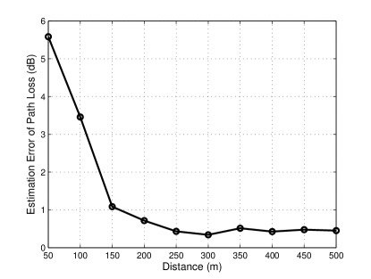
Figure 3: Estimation error vs. the distance between PU and BS

Figure 4: Locations of SU, PU and BS

Figure 5: Estimation error vs. PU location $(r_{1}=100m,400m)$

The performance of the method to estimate the path loss between PU and SU depends on the locations of SU, PU and BS. The locations in this simulation are shown in Fig. 4, where SU (marked as circle) is placed at $(-100,0)$ and $(-400,0)$, which stand for the cases of SU close to and far from BS, respectively. PU (marked as square) is confined at one of the three circles with radius $r_{0}$ equal to $100$ m, $250$ m and $400$ m, respectively. For each location of SU, the performance of the path loss estimation method is evaluated when PU moves along each of the three circles.

Fig. 5 shows the relation of the estimation error of the path loss between PU and SU versus the locations of PU when SU is located at different places. It can be seen that the estimation error is always below $2.7$ dB no matter where SU and PU are located, which indicates that our proposed path loss estimation method is very effective and applicable. It is also seen that the estimation error is always smaller when PU is far away from BS ($r_{0}=250$ m and $400$ m) than that when PU is close to BS ($r_{0}=100$ m). Two factors contribute to this. First, when PU is far away from BS, the estimation error of the path loss between BS and PU in the first step is smaller (see Fig. 3). So the performance of the method to estimate the path loss between PU and SU in the second step is better. Second, the PU transmission power is large when PU is far away from BS. So the SU received power is large correspondingly, which results in high received SINR and low estimation error.

VI Conclusions

This paper has proposed a novel non-cooperative path loss estimation method. In this method, SU independently derives the PDF and statistics of PU transmission power by exploiting the channel statics and broadcasted AMC mode information, and estimates the path loss between itself and PU by exploiting the relation among transmission power, received power and path loss. This method does not need any information exchange between SU and PU and does not make any impact on the communications in the macrocell. For the two-tier network whose primary tier is WiMAX or LTE, this method is compatible with the primary tier network completely and does not require any modification to the existing standard, which increases the applicability of the proposed method in real systems significantly. Simulation results show that our proposed method can estimate the path loss between PU and SU effectively no matter where SU and PU are located.

The proposed non-cooperative path loss estimation method is also applicable to other geography-overlapped and spectrum-shared two-tier networks, such as a traditional network co-existing with cognitive networks, etc.

Future work includes the research on the relationship between the performance and the number of observed samples I.

References

- [1] V. Chandrasekhar, J. Andrews, and A. Gatherer, “Femtocell networks: a survey,” IEEE Communications Magazine, vol. 46, pp. 59-67, 2008.
- [2] S. Haykin, “Cognitive radio: brain-empowered wireless communications,” IEEE Journal on Selected Areas in Communications, vol. 23, pp. 201-220, 2005.
- [3] H. Jiang, L. Lai, R. Fan, and H. V. Poor, “Optimal selection of channel sensing order in cognitive radio,” IEEE Transactions on Wireless Communications, vol. 8, no. 1, pp. 297-307, Jan. 2009.
- [4] R. Fan and H. Jiang, “Channel sensing-order setting in cognitive radio networks: A two-user case,” IEEE Transactions on Vehicular Technology, vol. 58, no. 9, pp. 4997-5008, Nov. 2009.
- [5] A. CORPORATION, “Method and Apparatus for Determining Path Loss by Active Signal Detection,” US Patent, PCT/US2006/017517, May 17, 2006.
- [6] J. P. Carlson and J. Arpee, “Method and Apparatus for determining path loss by combining geolocation with interference suppression,” US Patent, 434754, May 17, 2006.
- [7] I. T. Corporation, “Path loss measurements in wireless communications,” US Patent, 731457, December 9, 2003.
- [8] MOTOROLA, “System and method for using per-packet receive signal strength indication and transmit power levels to compute path loss for a link for use in layer II routing in a wireless communication network,” US Patent, 360075, Feb. 23, 2006.
- [9] J. Proakis, Digital Communication. MacGraw-Hill, 2001.
- [10] S. M. Kay, Fundamentals of Statistical Signal Processing: Estimation Theory. Prentice Hall, 1993.
- [11] Femto Forum Working Group 2 Document, “OFDMA Interference Study: Evaluation Methodology Document,” March 2009.