Nonrelativistic collisionless shocks in weakly magnetized electron–ion plasmas: two-dimensional particle-in-cell simulation of perpendicular shock

Abstract

A two-dimensional particle-in-cell simulation is performed to investigate weakly magnetized perpendicular shocks with a magnetization parameter of $\sigma=6\times 10^{-5}$, which is equivalent to a high Alfvén Mach number $M_{\mathrm{A}}$ of $\sim 130$. It is shown that current filaments form in the foot region of the shock due to the ion-beam–Weibel instability (or the ion filamentation instability) and that they generate a strong magnetic field there. In the downstream region, these current filaments also generate a tangled magnetic field that is typically 15 times stronger than the upstream magnetic field. The thermal energies of electrons and ions in the downstream region are not in equipartition and their temperature ratio is $T_{\mathrm{e}}/T_{\mathrm{i}}\sim 0.3-0.4$. Efficient electron acceleration was not observed in our simulation, although a fraction of the ions are accelerated slightly on reflection at the shock. The simulation results agree very well with the Rankine–Hugoniot relations. It is also shown that electrons and ions are heated in the foot region by the Buneman instability (for electrons) and the ion-acoustic instability (for both electrons and ions). However, the growth rate of the Buneman instability is significantly reduced due to the relatively high temperature of the reflected ions. For the same reason, ion–ion streaming instability does not grow in the foot region.

1. Introduction

A large volume of the universe (including interstellar and intergalactic space) is filled with hot, tenuous plasmas. Coulomb collisions between charged particles rarely occur in these plasmas and the plasma dynamics are dominated by collective phenomena involving particles and electromagnetic fields (e.g., plasma oscillations). Hence, such plasmas are known as collisionless plasmas. Even in collisionless plasmas, some kinds of “shocks” occur. These shocks generally have very complex formation mechanisms that involve various kinetic processes, including electrostatic instabilities, electromagnetic instabilities, and compression of background magnetic fields. The shocks driven in supernova remnants (SNRs) are considered to be collisionless ones.

SNR shocks propagate in the interstellar medium, which has weak magnetic fields of typically $\sim 3\mu$G. In the context of shocks in magnetized plasmas, the strength of the magnetic field, $B_{0}$, is frequently expressed in terms of the magnetization parameter or the sigma parameter, which is defined as the ratio of the magnetic energy density to the bulk kinetic energy density of the upstream plasma (both are measured in the shock rest frame). For nonrelativistic cases, it is given by

$$\sigma\equiv\frac{B_{0}^{2}/8\pi}{n_{\mathrm{e0}}(m_{\mathrm{e}}+m_{\mathrm{i}})V_{\mathrm{sh}}^{2}/2}=M_{\mathrm{A}}^{-2},$$ (1)

where $n_{\mathrm{e0}}$ is the electron number density in the upstream plasma, $m_{\mathrm{e}}$ is the electron mass, $m_{\mathrm{i}}$ is the ion mass, $V_{\mathrm{sh}}$ is the shock speed, and $M_{\mathrm{A}}$ is the Alfvén Mach number. For example, for the shock in SN1006 (except the North-West region), $n_{\mathrm{e0}}\sim 0.05$ cm^-3 and $V_{\mathrm{sh}}\sim 4900$ km s^-1 were inferred (Acero et al., 2007) so that $\sigma\sim 4\times 10^{-5}$. The recently discovered ‘youngest’ SNR G1.9+0.3 is considered to have a shock velocity of $V_{\mathrm{sh}}\sim 14,000$ km s^-1 (Reynolds et al., 2008); assuming that $n_{\mathrm{e0}}\sim 0.1$ cm^-3 gives $\sigma\sim 2\times 10^{-6}$. The sigma generally lies in the range $10^{-6}<\sigma<10^{-3}$ for shocks in young SNRs; these shocks are thus very low-$\sigma$ shocks (or, equivalently, very high Alfvén Mach number shocks).

Magnetized shocks have been extensively investigated, especially perpendicular shocks in which the background magnetic field is perpendicular to the shock normal. The structure of perpendicular shocks in the supercritical regime ($M_{\mathrm{A}}>M_{\mathrm{A}}^{*}$, where $M_{\mathrm{A}}^{*}\sim 3$) is known to some extent: a fraction of the incoming ions are reflected at the shock front (called the ‘ramp’) and the reflected ions form a slightly dense region, referred to as the ‘foot’, in front of the ramp. The ions also accumulate immediately behind the ramp and generate a strong magnetic field there, which is called the (magnetic) ‘overshoot’. Over the last decade, one-dimensional (1D) particle-in-cell (PIC) simulations that can model the kinetic dynamics of both electrons and ions have been performed to investigate high-Mach-number perpendicular shocks (e.g., Shimada & Hoshino, 2000; Schmitz et al., 2002; Scholer et al., 2003). Recently, several two-dimensional (2D) simulations have also been performed (e.g., Umeda et al., 2008; Amano & Hoshino, 2009; Lembège et al., 2009). However, most simulations have been conducted for relatively strong background magnetic fields ($\sigma>5\times 10^{-3}$ or $M_{\mathrm{A}}<15$). It is thus desirable to perform simulations for weaker background fields.

On the other hand, it was recently demonstrated that certain kinds of collisionless shocks can occur even in unmagnetized plasmas at relativistic shock speeds by performing two- or three-dimensional (3D) PIC simulations (Kato, 2007; Spitkovsky, 2008; Chang et al., 2008). In these shocks, the beam–Weibel instability (or filamentation instability) is driven in the transition region of the shocks between the counterstreaming electron–positron beams in pair plasmas or between the counterstreaming ion beams in electron–ion plasmas and generates strong magnetic fields there. These generated fields provide an effective dissipation mechanism for collisionless shock formation and are hence often referred to as “Weibel-mediated shocks.” [Note that the beam–Weibel instability is driven by the counterstreaming beams (c.f. Fried, 1959) and it differs from the ordinary Weibel instability, which is driven by a temperature anisotropy (Weibel, 1959) (see also Davidson et al. (1972)).] These shocks can be driven by relativistic phenomena, such as gamma-ray bursts and their afterglows (Medvedev & Loeb, 1999; Brainerd, 2000), jets from active galactic nuclei, and pulsar winds (Kazimura et al., 1998). It was also shown in our previous paper (Kato & Takabe, 2008) that this kind of shock can form in unmagnetized electron–ion plasmas even at nonrelativistic speeds. The beam–Weibel instability can also be important in weakly magnetized shocks. As was shown in our previous paper, the magnetic field generated by the ion beam–Weibel instability reaches a few percent of the upstream bulk kinetic energy and this value is much higher than the background magnetic field around typical SNR shocks. Therefore, the ion beam–Weibel instability may play an important role in the formation of weakly magnetized shocks. Magnetized shocks have been extensively investigated by 1D simulations. However, 1D simulations cannot consider the beam–Weibel instability because its wave vector is perpendicular to the flow direction. Therefore, it is essential to perform multidimensional simulations to investigate the formation process of weakly magnetized nonrelativistic shocks.

Collisionless shocks are also considered sites of particle acceleration. In particular, cosmic-rays with energies below $10^{15}$ eV are considered to be accelerated in SNR shocks. Indeed, recent X-ray observations revealed that electrons are accelerated to energies of $\sim 10^{14}$ eV in several young SNRs (Koyama et al., 1995; Long et al., 2003; Bamba et al., 2003). It is widely accepted that first-order Fermi acceleration or diffusive shock acceleration is the acceleration mechanism (e.g., Drury, 1983; Blandford & Eichler, 1987). However, it is currently not possible to determine the fraction of thermal plasma particles that are injected into the diffusive shock acceleration process (this is known as the injection problem). For electron injection in quasi-perpendicular shocks, the shock surfing acceleration has been investigated as an injection mechanism or even as an efficient acceleration mechanism (Hoshino, 2001; McClements et al., 2001; Hoshino & Shimada, 2002). However, several researchers have recently shown that the shock surfing acceleration process is in fact inefficient in 2D (e.g., Dieckmann & Shukla, 2006; Ohira & Takahara, 2007; Umeda et al., 2008) and that it is efficient in 1D because of the symmetry of the system. Instead, Amano & Hoshino (2009) showed that another acceleration process can operate in 2D in which a fraction of electrons are reflected in the foot region by small-scale electrostatic waves generated by the Buneman instability. They are then accelerated by the motional electric field as well as being directly accelerated by the electric field when they resonate with the electrostatic waves. Electrons can be accelerated up to about the upstream ion bulk energy by this mechanism. Thus, multidimensional effects can play an essential role in the acceleration/injection mechanism.

In addition, collisionless shocks can be sites of magnetic field amplification/generation. Recent X-ray observations suggest that magnetic fields of the order of hundreds of microgauss or even milligauss may be generated in the vicinity of SNR shocks (Vink & Laming, 2003; Völk et al., 2005; Uchiyama, 2007). Several mechanisms have been proposed for this magnetic field amplification, including a nonresonant instability driven by high-energy particles accelerated in shocks (Bell, 2004) and magnetohydrodynamic turbulence behind shocks (Giacalone & Jokipii, 2007; Inoue et al., 2009). The mechanism may be related with the microscopic kinetic processes associated with shock formation itself; it should in principle be possible to investigate this by performing large-scale PIC simulations.

In this study, we investigate the formation and structure of perpendicular shocks for very low $\sigma$ and the processes responsible for particle acceleration and magnetic field generation by performing 2D PIC simulation, which can appropriately model the beam–Weibel instability. Because of the capability of the computer, we used a reduced ion-to-electron mass ratio and a shock speed ($V_{\mathrm{sh}}\sim 0.3c$, where $c$ is the speed of light) that is much higher than realistic ones for SNRs ($V_{\mathrm{sh}}\sim 0.01c$) in the simulation.

2. METHOD

We investigated collisionless shocks in electron–ion plasmas with weak background magnetic fields by performing a 2D PIC simulation. The simulation code is a relativistic, electromagnetic, PIC code with two spatial and three velocity dimensions developed based on a standard method described by Birdsall & Langdon (1991). The basic equations of the simulation are Maxwell’s equations and the (relativistic) equation of motion for particles. In the following, we regard the simulation plane as the $x-y$ plane and we take the $z$-axis to be perpendicular to the plane. We take $\tau=\omega_{\mathrm{pe}}^{-1}$ to be the unit of time and the electron skin depth $\lambda_{\mathrm{e}}=c\omega_{\mathrm{pe}}^{-1}$ to be the unit of length, where $\omega_{\mathrm{pe}}\equiv(4\pi n_{\mathrm{e0}}e^{2}/m_{\mathrm{e}})^{1/2}$ is the electron plasma frequency defined for the electron number density in the far upstream region, $n_{\mathrm{e0}}$. The units for electric and magnetic fields are $E_{*}=B_{*}=c(4\pi n_{\mathrm{e0}}m_{\mathrm{e}})^{1/2}$.

In the simulation, a collisionless shock is driven according to the “injection method.” There are two walls, one on the left-hand side (smaller $x$) and the other on the right-hand side (larger $x$) of the simulation box and these walls reflect particles specularly. Initially, both electrons and ions are loaded uniformly in the region between the two walls with a bulk velocity of $V$ in the $+x$-direction. The electrons and ions have equal temperatures in the upstream region. In the early stages of the simulation, particles near the right wall are reflected by the wall and then interact with incoming particles (i.e., the upstream plasma). This interaction generates some instability and eventually a collisionless shock forms. The frame of the simulation is the rest frame of the shock downstream; the shock propagates from right to left in the downstream rest frame.

We consider a perpendicular shock in this paper; the initial magnetic field, $B_{0}$, is in the $y$-direction (i.e., in the plane) and its strength is determined by the sigma. However, since the shock speed is unknown before performing the simulation, in the following, the sigma is defined in the simulation frame with an upstream bulk velocity $V$ instead of the shock speed $V_{\mathrm{sh}}$ as

$$\tilde{\sigma}\equiv\frac{B_{0}^{2}/8\pi}{n_{\mathrm{e0}}(m_{\mathrm{e}}+m_{\mathrm{i}})V^{2}/2};$$ (2)

however, the difference between these two sigmas is not large. With this definition of the sigma, the magnetic field strength in the simulation frame is given by $B_{0}=\left[(1+m_{\mathrm{i}}/m_{\mathrm{e}})\tilde{\sigma}\right]^{1/2}(V/c)B_{*}$. The initial electric field, $E_{0}$, is determined so that it vanishes in the plasma rest frame (i.e., the upstream frame); this requirement causes the motional electric field in the simulation frame, $E_{0}=-VB_{0}/c$, in the $z$-direction. The boundary conditions for both the particles and the electromagnetic field are periodic in the $y$-direction.

3. RESULTS AND ANALYSIS

We performed a simulation for a sigma of $\tilde{\sigma}=10^{-4}$. As mentioned above, we use a reduced ion mass of $m_{\mathrm{i}}=30m_{\mathrm{e}}$ and a bulk velocity of $V=0.25c$. The grid size is $N_{x}\times N_{y}=16384\times 1024$ and there are $\sim 40$ particles per cell per species. The physical dimensions of the simulation box are $L_{x}\times L_{y}=3200\lambda_{\mathrm{e}}\times 200\lambda_{\mathrm{e}}$ and thus the size of a cell is $\Delta x=\Delta y\sim 0.2\lambda_{\mathrm{e}}$. The electron and ion temperatures are equal and are given by $k_{\mathrm{B}}T/m_{\mathrm{e}}c^{2}=1.25\times 10^{-3}$, where $k_{\mathrm{B}}$ is the Boltzmann constant. The thermal velocities are thus given by $a_{\mathrm{e}}=(2k_{\mathrm{B}}T/m_{\mathrm{e}})^{1/2}=0.05c$ for the electrons and $a_{\mathrm{i}}=9.13\times 10^{-3}c$ for the ions. For these parameters, we have $\omega_{\mathrm{ce}}/\omega_{\mathrm{pe}}=B_{0}/B_{*}\sim 1.4\times 10^{-2}$, the Alfvén speed $v_{\mathrm{A}}\sim 2.5\times 10^{-3}c$ (thus, $\tilde{M_{\mathrm{A}}}\equiv V/v_{\mathrm{A}}=100$), and the plasma beta $\beta\sim 26$ (i.e., it is a high-beta plasma). The Larmor radii of the electrons and ions calculated for the background field and the upstream bulk velocity are $r_{g,e}=18\lambda_{\mathrm{e}}$ and $r_{g,i}=535\lambda_{\mathrm{e}}$, respectively.

3.1. Overall structure

Figure 1 shows the time evolution of the ion number density averaged over the $y$-direction. The shock transition region, or the “shock front”, appears as a steep increase in the number density. The shock structure and its propagation speed abruptly change around $\omega_{\mathrm{pe}}t\sim 3000$. This is because the shock structure undergoes a transition from an unmagnetized shock to a magnetized shock. Indeed, the structure for $\omega_{\mathrm{pe}}t<2000$ is essentially the same as those of Weibel-mediated shocks in unmagnetized plasmas (Kato & Takabe, 2008), as discussed below. The transition time is of the order of the gyration time of the ions in the background field, $T_{g}\equiv 2\pi/\omega_{\mathrm{ci}}$, where $\omega_{\mathrm{ci}}\equiv eB_{0}/m_{\mathrm{i}}c$ is the ion cyclotron frequency. For the unmagnetized shock ($1500<\omega_{\mathrm{pe}}t<2000$), the shock speed measured in the downstream frame is $V_{\mathrm{sh,d}}\sim-0.16c$. For the magnetized shock ($\omega_{\mathrm{pe}}t>4000$), it becomes $V_{\mathrm{sh,d}}\sim-0.08c$ and that in the upstream frame and the Alfvén Mach number are given by $V_{\mathrm{sh}}\sim-0.33c$ and $M_{\mathrm{A}}\sim 130$, respectively. Thus, the sigma defined for the shock velocity is given by $\sigma=5.9\times 10^{-5}$ in this case. The shock speeds obtained here may have small uncertainties because they were obtained by eye-fitting the figure and also they may not be in the steady state yet. Since the formation of an unmagnetized shock is a consequence of the initial conditions and we are interested in the magnetized shock in this study, we mainly focus on the magnetized shock below. We discuss the unmagnetized shock at the end of this section.

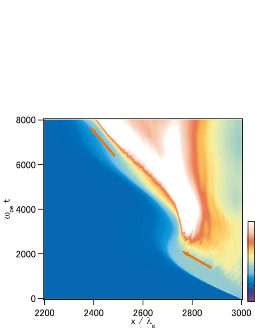
Figure 1.— Time development of the ion number density averaged over the $y$-direction for the simulation with an upstream bulk velocity of $V=0.25c$ and a sigma parameter of $\tilde{\sigma}=10^{-4}$. The color indicates the number density normalized by that in the far upstream $n_{\mathrm{e0}}$. The horizontal and vertical axes respectively represent $x$ (in units of electron skin depth $\lambda_{\mathrm{e}}$) and time (in units of the electron plasma time $\omega_{\mathrm{pe}}^{-1}$). The shock structure and its propagation speed change abruptly around $\omega_{\mathrm{pe}}t\sim 3000$ due to the transition from an unmagnetized shock to a magnetized shock. The arrows indicate the obtained shock speeds for the unmagnetized shock ($V_{\mathrm{sh,d}}\sim-0.16c$) and the magnetized shock ($V_{\mathrm{sh,d}}\sim-0.08c$).

Figure 1 shows that the shock wave almost reaches steady state near the end of the simulation ($\omega_{\mathrm{pe}}t\sim 8000$). Figure 2 shows the ion number density at $\omega_{\mathrm{pe}}t=8000$. (Hereafter, we discuss the results at this time unless otherwise stated.) The upstream plasma flows from left to right and moves through the transition region ($2350<x/\lambda_{\mathrm{e}}<2550$) and then reaches the downstream state. (The structure in Fig. 1 in $x>2700\lambda_{\mathrm{e}}$ is an artifact due to the boundary and so in the following we discuss the structure in $x<2700\lambda_{\mathrm{e}}$.) Note that there are filamentary structures, which cannot be observed in 1D simulations, in the upstream leading edge of the shock transition region ($x\sim 2400\lambda_{\mathrm{e}}$). The filament radius is typically approximately equal to the ion inertial length, which is the same as those in the “Weibel-mediated” shocks in unmagnetized electron–ion plasmas (Kato & Takabe, 2008). Then, behind them, there is a highly fluctuating high-density region. In the downstream region ($x>2550\lambda_{\mathrm{e}}$), the number density becomes almost homogeneous.

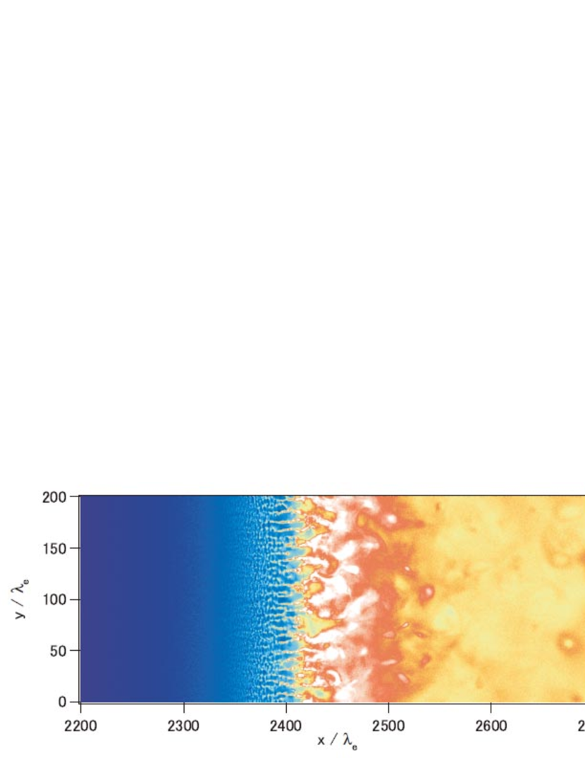
Figure 2.— Ion number density at $\omega_{\mathrm{pe}}t=8000$. The horizontal and vertical axes represent $x$ and $y$, respectively. The left- and right-hand sides are upstream and downstream of the shock, respectively. Many filamentary structures can be seen in the shock transition region ($2350<x/\lambda_{\mathrm{e}}<2550$).

Figures 3(a) and (b) show profiles of the ion number density and the magnetic field strength averaged over the $y$-direction, respectively. It shows that the number density increases rapidly in the transition region and after the transition region it approaches $\sim 4$ times the upstream value. Figure 3(b) shows the root mean square of each magnetic field component together with the total magnetic field strength. This structure is similar to the well-known structure of supercritical perpendicular shocks in 1D; the ‘ramp’ is at $x\sim 2400\lambda_{\mathrm{e}}$ and there is an extended ‘foot’ region in $x<2400\lambda_{\mathrm{e}}$ as well as an ‘overshoot’ region in $2400<x/\lambda_{\mathrm{e}}<2470$. It is evident that strong magnetic fields are generated in both the shock transition region (or the overshoot) and the downstream region. The energy density of the magnetic field reaches $\sim 15\%$ of the upstream bulk kinetic energy density (measured in the downstream rest frame) in the shock transition region and $\sim 2\%$ in the downstream region. It is notable that $B_{x}$ and $B_{z}$, which are generated by the current filaments of the ion-beam–Weibel instability (see below), are comparable with $B_{y}$, which is mostly generated by the upstream background field. These $B_{x}$ and $B_{z}$ fields as well as the $B_{y}$ field contribute to the dissipation of the shock. Since these filaments and the magnetic field are never generated in 1D simulations, the shock structure may differ significantly from those in 1D cases.

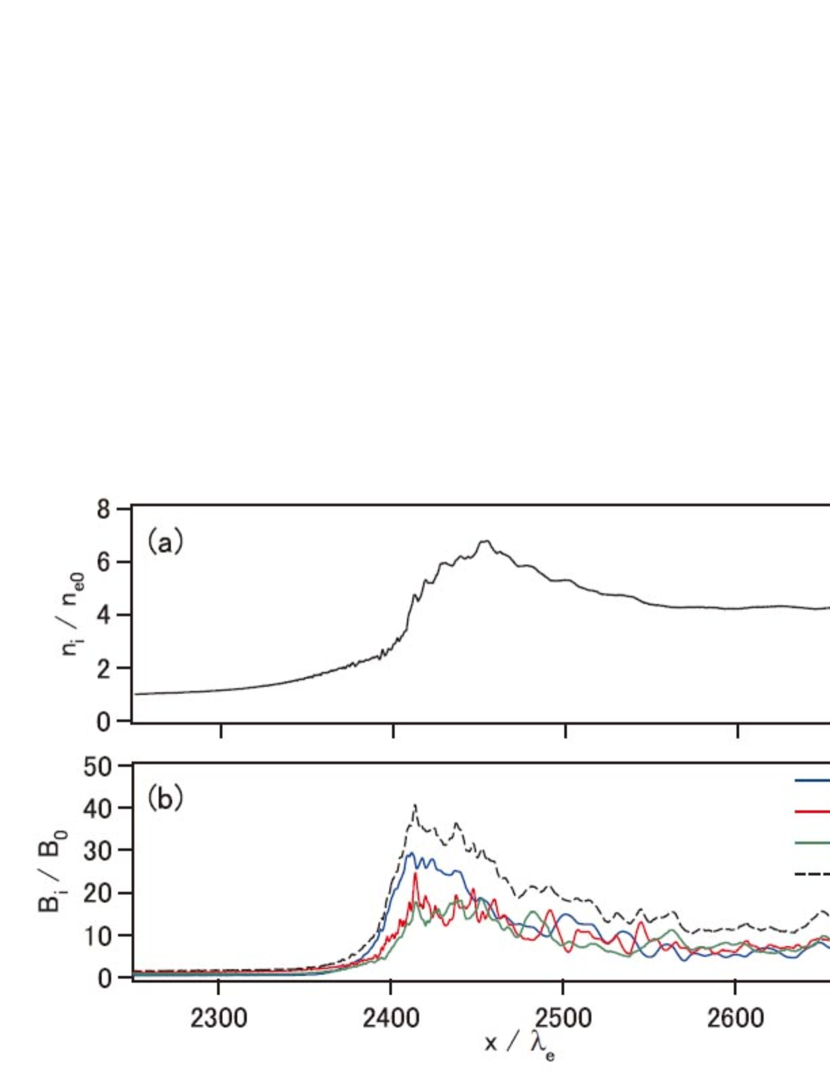
Figure 3.— Profiles of (a) the ion number density normalized by the upstream density $n_{\mathrm{e0}}$ and (b) the root mean square of each magnetic field component ($B_{x}$, blue curve; $B_{y}$, red curve; $B_{z}$, green curve) and that of the total strength ($|B|$, dashed black curve), where all the components are normalized by the upstream background field $B_{0}$.

Figure 4 shows phase-space plots of the electrons and the ions. Here, each component of the four velocities ($u_{j}=\gamma v_{j}/c$, where $j=x,y,z$ and $\gamma\equiv(1-v^{2}/c^{2})^{-1/2}$ is the Lorentz factor of the particle) are plotted as a function of the $x$-coordinate. Both electrons and ions from upstream are mostly dissipated and isotropically thermalized through the transition region ($2300\lambda_{\mathrm{e}}<x<2450\lambda_{\mathrm{e}}$). It is observed that a fraction of ions are reflected at $x\sim 2400\lambda_{\mathrm{e}}$ (i.e., the ramp) and then gyrate back downstream with slight acceleration forming the foot structure. This is a well-known characteristic of supercritical shocks and has been observed in many numerical simulations (e.g., Leroy, 1981; Burgess, 1989). In contrast, the electrons have no prominent substructures in phase space.

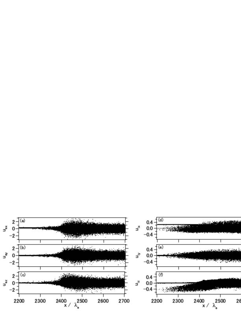
Figure 4.— Phase-space plots of electrons (left panel) and ions (right panel). The (from top to bottom) $x$, $y$, and $z$ components of the four velocities are shown in each panel. Both species are mostly thermalized within the shock transition region. A fraction of the incoming ions are reflected at $x\sim 2400\lambda_{\mathrm{e}}$.

3.2. Foot dynamics

Figure 5 shows the distribution of the ion kinetic energy measured in the upstream frame, $E_{\mathrm{kin,u}}=(\gamma_{\mathrm{u}}-1)mc^{2}$, where $\gamma_{\mathrm{u}}$ is the particle Lorentz factor measured in the upstream frame, as a function of the $x$-coordinate (in the downstream frame) at $\omega_{\mathrm{pe}}t=8000$. In this figure, the incoming and reflected ions in the foot region ($2200<x/\lambda_{\mathrm{e}}<2400$) can be clearly distinguished from each other using a threshold energy of, for example, $E_{\mathrm{kin,u}}/m_{\mathrm{e}}c^{2}=1$: the reflected ions with $E_{\mathrm{kin,u}}/m_{\mathrm{e}}c^{2}>1$ and the incoming ions with $E_{\mathrm{kim,u}}/m_{\mathrm{e}}c^{2}<1$. The reflected ions are further divided into two populations: those streaming upstream measured in the shock rest frame and those streaming downstream. Thus, we can investigate the foot dynamics on the basis of a simple fluid model that consists of a single electron fluid and three ion fluids (incoming ions, reflected ions streaming upstream, and those streaming downstream), which is similar to the model used in Leroy (1983). For convenience, we denote the electrons, the incoming ions, the reflected ions streaming upstream, and those streaming downstream by the symbols e, I, R_-, and R₊, respectively.

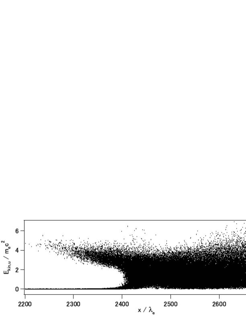
Figure 5.— Kinetic energy of the ions measured in the upstream frame.

Figures 6(a) and (b) show the mean velocity of each fluid component in the $x$- and $z$-directions and Fig. 6(c) shows the number densities normalized by the upstream number density. In the downstream region ($x>2400\lambda_{\mathrm{e}}$), only the values for all the ions are shown because classifying the ions by the above method is meaningless in that region. It shows that the mean velocities and the number density of all electrons (thick curves) and for all ions (dashed white curves) agree well with each other in both the upstream and downstream regions, indicating that the massless electron fluid model (Leroy, 1983) holds well, at least on average, even in this high Mach number and low ion-to-electron mass ratio case.

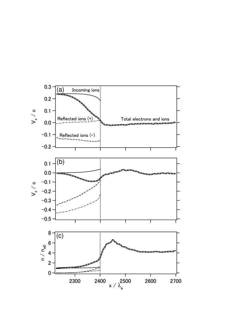
Figure 6.— Profiles of the mean velocities in the (a) $x$- and (b) $z$-directions, and (c) the mean number densities normalized by the upstream number density.

3.2.1 Electrostatic instabilities and heating

The local temperatures of the respective components were calculated using the mean velocities obtained above and they are plotted in Fig. 7. It shows that in the foot region, the electrons are heated in two steps: the first step in $x\leq 2350\lambda_{\mathrm{e}}$ (region 1) and the second step in $2350\leq x/\lambda_{\mathrm{e}}\leq 2400$ (region 2). The incoming ions are also heated in region 2. This sequential electron heating process together with the ion heating suggests that the model for very high Mach number shocks proposed by Papadopoulos (1988) is valid in the foot region, in which the incoming electrons are first heated by the Buneman instability (Buneman, 1958) for reflected ions (Auer et al., 1971) and subsequently, after the electrons have been heated to a certain temperature, they are further heated by the ion-acoustic instability for incoming ions. The latter instability can also heat the ions. This process has been studied by Cargill & Papadopoulos (1988) for $M_{\mathrm{A}}\sim 50$ and $500$ with hybrid simulations with a phenomenological resistivity and also by Shimada & Hoshino (2000) for $M_{\mathrm{A}}\sim 10.5$ with 1D PIC simulations.

Figure 7.— Temperature profile of each component. Both incoming electrons (thick solid curve) and incoming ions (thin solid curve) are heated in the foot region ($x<2400\lambda_{\mathrm{e}}$).

This heating process is expected to operate in very high Mach number shocks and so it should also operate in the present case ($M_{\mathrm{A}}\sim 130$). Figure 8 shows several quantities of each ion component obtained from Figs. 6 and 7; specifically, it shows profiles of the mean velocity relative to the electron velocity in the $x$-direction, the electron-to-ion temperature ratio, and the number density normalized by the local electron number density $n_{\mathrm{e}}(x)$. In region 1 ($x<2350\lambda_{\mathrm{e}}$), the reflected ions streaming upstream have a significantly higher velocity relative to the electrons than the electron thermal velocity. On the other hand, in region 2 ($x>2350\lambda_{\mathrm{e}}$), the electron-to-ion temperature ratio for the incoming ions increases to a large value and also the incoming ion velocity relative to the electron velocity becomes large due to the large deceleration of the electrons [see Fig. 6(a)] so that it becomes higher than the ion-acoustic speed, $c_{\mathrm{s}}\equiv(k_{\mathrm{B}}T_{\mathrm{e}}/m_{\mathrm{i}})^{1/2}$. These conditions are indeed preferable to the Buneman instability in region 1 and the ion-acoustic instability in region 2.

Figure 8.— Profiles of the quantities in the foot region for incoming ions (thin solid curves), reflected ions streaming upstream (dashed curves), and reflected ions streaming downstream (dot-dashed curves). (a) The velocities relative to the electron velocity in the $x$-direction (absolute values). The electron thermal velocity (thick solid curve) and the ion-acoustic speed (thick dotted curve) are also shown. (b) The electron-to-ion temperature ratios. (c) The number densities normalized by the local electron number density, $n_{\mathrm{e}}(x)$.

Here, we show the instabilities that operate in the foot region by performing local linear analysis with the fluid quantities (namely, the mean velocities, the number densities, and the temperatures shown in Figs. 6 and 7). Approximating the distribution of each component as a Maxwellian distribution,

$$f_{0}^{(\mathrm{s})}(v_{x},v_{y},v_{z})=\frac{n_{\mathrm{s}}}{\pi^{3/2}a_{\mathrm{s}}^{3}}\exp\left[-\frac{(v_{x}-V_{\mathrm{s},x})^{2}+v_{y}^{2}+(v_{z}-V_{\mathrm{s},z})^{2}}{a_{\mathrm{s}}^{2}}\right],$$ (3)

where $\mathrm{s}=(\mathrm{e,I,R_{-},R_{+}})$, $n_{\mathrm{s}}$ is the number density, $V_{\mathrm{s},x}$ and $V_{\mathrm{s},z}$ are the streaming velocities in the $x$- and $z$-directions respectively, and $a_{\mathrm{s}}=(2k_{\mathrm{B}}T_{\mathrm{s}}/m_{\mathrm{s}})^{1/2}$ is the thermal velocity. We solve the following dispersion relation for the electrostatic mode with the wavevector in the $x$-direction:

$$k_{x}^{2}+2\sum_{\mathrm{s}}k_{\mathrm{Ds}}^{2}(1+\zeta_{\mathrm{s}}Z(\zeta_{\mathrm{s}}))=0,$$ (4)

where

$$k_{\mathrm{Ds}}\equiv\omega_{\mathrm{ps}}/a_{\mathrm{s}},\quad\omega_{\mathrm{ps}}\equiv\left(\frac{4\pi n_{\mathrm{s}}q_{\mathrm{s}}^{2}}{m_{\mathrm{s}}}\right)^{1/2},$$ (5)

and

$$\zeta_{\mathrm{s}}=\zeta_{\mathrm{s}}(\omega,k_{x})\equiv(\omega-k_{x}V_{\mathrm{s}})/k_{x}a_{\mathrm{s}}.$$ (6)

The function $Z(\zeta)$ is the plasma dispersion function (Fried & Conte, 1961) defined by

$$Z(\zeta)\equiv\pi^{-1/2}\int_{-\infty}^{\infty}\frac{e^{-z^{2}}}{z-\zeta}dz.$$ (7)

Table 1 summarizes some quantities used in the following analysis.

Table 1 Quantities obtained from the simulation. The units for the $x$-coordinate, the velocity, the number density, and the temperature are $\lambda_{\mathrm{e}}$, $c$, $n_{\mathrm{e0}}$, and $m_{\mathrm{e}}c^{2}$, respectively.

$x$	$V_{\mathrm{e},x}$	$V_{\mathrm{e},z}$	$n_{\mathrm{e}}$	$T_{\mathrm{e}}$	$V_{\mathrm{I},x}$	$V_{\mathrm{I},z}$	$n_{\mathrm{I}}$	$T_{\mathrm{I}}$	$V_{\mathrm{R-},x}$	$V_{\mathrm{R-},z}$	$n_{\mathrm{R-}}$	$T_{\mathrm{R-}}$	$V_{\mathrm{R+},x}$	$V_{\mathrm{R+},z}$	$n_{\mathrm{R+}}$	$T_{\mathrm{R+}}$
$2300$	$0.20$	$-0.042$	$1.1$	$2.5\times 10^{-3}$	$0.24$	$3.3\times 10^{-3}$	$0.99$	$1.3\times 10^{-3}$	$-0.14$	$-0.27$	$0.069$	$0.090$	$4.6\times 10^{-3}$	$-0.39$	$0.084$	$0.14$
$2350$	$0.11$	$-0.089$	$1.6$	$8.6\times 10^{-3}$	$0.23$	$0.013$	$1.0$	$1.8\times 10^{-3}$	$-0.15$	$-0.19$	$0.37$	$0.12$	$5.5\times 10^{-3}$	$-0.34$	$0.26$	$0.19$
$2375$	$0.062$	$-0.093$	$2.1$	$0.033$	$0.22$	$0.023$	$1.0$	$4.6\times 10^{-3}$	$-0.16$	$-0.15$	$0.68$	$0.14$	$0.013$	$-0.32$	$0.38$	$0.22$

We use here the dispersion relation for unmagnetized plasmas given by Eq. (4) instead of that for magnetized plasmas because the magnetic field is sufficiently weak in the present case; the condition for the unmagnetized approximation is given by $k^{2}\gg k_{\mathrm{cs}}^{2}$ where $k_{\mathrm{cs}}\equiv\sqrt{2}|\omega_{\mathrm{cs}}|/a_{\mathrm{s}}$; in other words, for all species, the wavelength is much smaller than the Larmor radius defined for the thermal velocity. As shown below, the wavenumbers of the instabilities are typically $kc/\omega_{\mathrm{pe}}>3$ and $k_{\mathrm{cs}}c/\omega_{\mathrm{pe}}$ is $\sim 0.5$ for electrons, $\sim 0.15$ for incoming ions, and $\sim 0.01$ for reflected ions in the foot region. Therefore, the unmagnetized approximation can be used in this case.

When performing the linear analysis with the local quantities at $x=2300\lambda_{\mathrm{e}}$, we found an unstable electrostatic mode whose wavenumber ($k_{x}\sim 3.5\omega_{\mathrm{pe}}/c$) and frequency ($\omega^{\prime}\sim 0.048\omega_{\mathrm{pe}}$ in the rest frame of the reflected ions $R_{-}$) are similar to those of the Buneman instability between electrons and reflected ions streaming upstream ($k_{x}\sim 2.9\omega_{\mathrm{pe}}/c$ and $\omega^{\prime}\sim 0.05\omega_{\mathrm{pe}}$ in the rest frame of $R_{-}$). However, the obtained growth rate ($\gamma\sim 0.0057\omega_{\mathrm{pe}}$) is one order of magnitude smaller than the typical growth rate of the Buneman instability ($\gamma\sim 0.087\omega_{\mathrm{pe}}$). This is because of the relatively high temperature of the reflected ions streaming upstream, $T_{R-}$, as is shown in Fig. 7, while the ordinary Buneman instability assumes that both species are cold. Figure 9 shows the maximum linear growth rates of this mode together with their wavenumbers calculated for the quantities at $x=2300\lambda_{\mathrm{e}}$ while varying $T_{R-}$. When $T_{R_{-}}$ approaches zero, the growth rate becomes large and approaches to a typical value for the Buneman instability. Thus, we regard this mode as a Buneman instability between the electrons and the reflected ions streaming upstream with a reduction in the growth rate due to the relatively high temperature of the reflected ions.

Figure 9.— (a) Maximum linear growth rates of the electrostatic mode and (b) the wave numbers at the maximum growth rates as functions of the temperature of the reflected ions streaming upstream, $T_{R-}$, calculated for the quantities obtained from the simulation at $x=2300\lambda_{\mathrm{e}}$ (except $T_{R-}$). Those for the original value of $T_{R-}$ in the simulation are indicated by the arrows.

On the other hand, we found another unstable electrostatic mode at $x\sim 2350\lambda_{\mathrm{e}}$. This mode has a maximum growth rate $\gamma_{\mathrm{max}}\sim 0.02\omega_{\mathrm{pe}}$ and a frequency $\omega\sim 0.52\omega_{\mathrm{pe}}$ at $k_{x}\sim 4.85\omega_{\mathrm{pe}}/c$. This leads to a phase velocity of $\sim-0.017c$ in the incoming ion rest frame. For the same parameters, the dispersion relation of the ion-acoustic instability (Ichimaru, 1973) between electrons and incoming ions gives $\gamma_{\mathrm{max}}\sim 0.015\omega_{\mathrm{pe}}$ at $k_{x}\sim 4.0\omega_{\mathrm{pe}}/c$ and a phase speed of $c_{\mathrm{s}}\sim-0.016c$ in the incoming ions rest frame. Both agree well with each other and thus we regard this mode as an ion-acoustic instability between electrons and incoming ions.

Figure 10 summarizes the results for this local linear analysis over the foot region. The Buneman instability develops upstream of the foot region ($x\leq 2325\lambda_{\mathrm{e}}$), whereas the ion-acoustic instability dominates downstream of the foot region ($x\geq 2325\lambda_{\mathrm{e}}$). This feature is consistent with the evolution of the electron and incoming ion temperatures shown in Fig. 7; the electrons are first heated by the Buneman instability and then both electrons and incoming ions are heated by the ion-acoustic instability. Note that there is a region where both instabilities can coexist ($2312\leq x/\lambda_{\mathrm{e}}\leq 2325$).

Figure 10.— (a) Maximum linear growth rates of the Buneman instability (filled circles) and the ion-acoustic instability (crosses) as functions of $x$. (b) The wave numbers at the maximum growth rates for the respective instabilities.

Since both the Buneman and the ion-acoustic instabilities are electrostatic modes, they are always associated with the charge density $\rho$ and can be investigated through it. Figures 11(a) and (b) show the charge density and its power spectrum in two rectangular areas in the foot region, namely $x\sim 2300\lambda_{\mathrm{e}}$ (where the Buneman instability dominates) and $x\sim 2350\lambda_{\mathrm{e}}$ (where the ion-acoustic instability dominates), respectively. The peak positions of these power spectra agree well with the wavenumbers for the maximum growth rates obtained by the linear theory shown in Fig. 10. Note that both spectra are not concentrated on the $k_{x}$-axis but extend in the $k_{y}$-direction. This results in the wavy appearance of both modes in real space (left panels) and is a well-known characteristic of both instabilities in multiple dimensions.

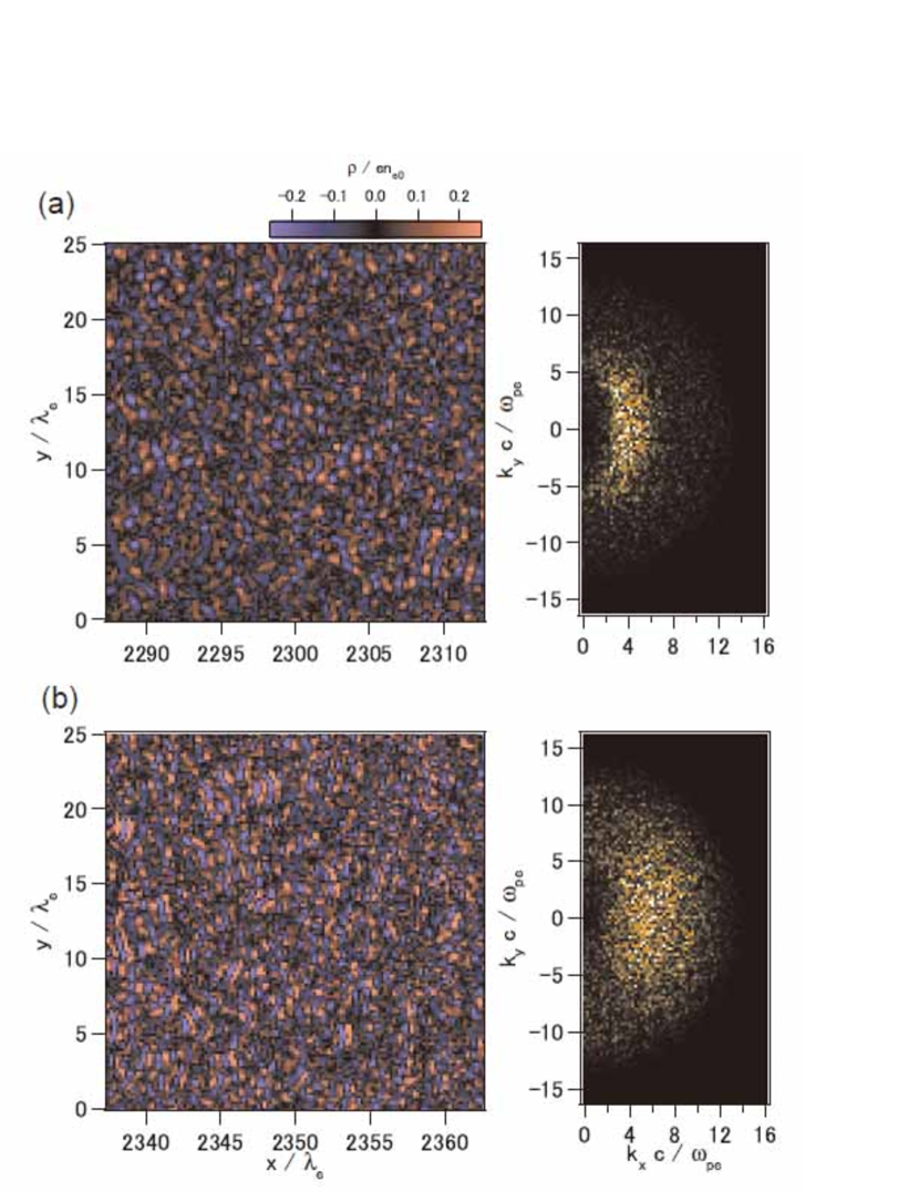
Figure 11.— Charge density (left panels) and its power spectrum (right panels): around (a) $x\sim 2300\lambda_{\mathrm{e}}$ and (b) $x\sim 2350\lambda_{\mathrm{e}}$. The portions where the power is strong are consistent with the linear theory of (a) the Buneman instability and (b) the ion-acoustic instability, respectively.

3.2.2 Filamentary structures

As mentioned above, the ion number density in the foot region (Fig. 2) contains many filamentary structures. Figure 12 shows that these filaments are associated with current filaments and filamentary magnetic fields. These filaments are similar to those observed in unmagnetized shocks, which are generated by the beam-Weibel instability.

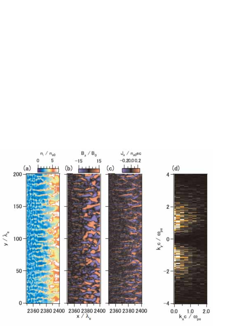
Figure 12.— (a) Ion number density, (b) magnetic field $B_{z}$, and (c) current density in the $x$-direction, $J_{x}$, around $x\sim 2375\lambda_{\mathrm{e}}$. (d) Power spectrum of $J_{x}$ calculated in the region $2362.5<x/\lambda_{\mathrm{e}}<2385.5$.

In our previous papers, we showed that the ion beam–Weibel instability develops and generates currents filaments even for nonrelativistic flow speeds (Kato & Takabe, 2008, 2010). Therefore, it is plausible that these filaments are generated by the ion beam-Weibel instability. To confirm this, we performed linear analysis in the same manner as that used to obtain Fig. 10 except that we here consider the electromagnetic modes with wavevectors in the $y$-direction. In the present case, since the wavenumber is too low to employ the unmagnetized approximation for electrons, we solve the following dispersion relation in the electron rest frame, which includes the effect of the magnetic field for the electrons (the ions are assumed to be unmagnetized):

$$\mathrm{det}\Lambda=0,$$ (8)

where

$$\Lambda_{xx} = 1-\left(\frac{kc}{\omega}\right)^{2}+\frac{1}{2}\left(\frac{\omega_{\mathrm{pe}}}{\omega}\right)^{2}\xi_{0}\left[Z(\xi_{1})+Z(\xi_{-1})\right]+\sum_{\mathrm{s}}\left(\frac{\omega_{\mathrm{ps}}}{\omega}\right)^{2}\left[\alpha_{\mathrm{s}}+2\tilde{V}_{\mathrm{s}x}^{2}(1+\alpha_{\mathrm{s}})\right],$$ (9)

$$\Lambda_{yy} = 1+2\left(\frac{\omega_{\mathrm{pe}}}{ka_{\mathrm{e}}}\right)^{2}\left[1+\xi_{0}Z(\xi_{0})\right]+2\sum_{\mathrm{s}}\left(\frac{\omega_{\mathrm{ps}}}{ka_{\mathrm{s}}}\right)^{2}(1+\alpha_{\mathrm{s}}),$$ (10)

$$\Lambda_{zz} = 1-\left(\frac{kc}{\omega}\right)^{2}+\frac{1}{2}\left(\frac{\omega_{\mathrm{pe}}}{\omega}\right)^{2}\xi_{0}\left[Z(\xi_{1})+Z(\xi_{-1})\right]+\sum_{\mathrm{s}}\left(\frac{\omega_{\mathrm{ps}}}{\omega}\right)^{2}\left[\alpha_{\mathrm{s}}+2\tilde{V}_{\mathrm{s}z}^{2}(1+\alpha_{\mathrm{s}})\right],$$ (11)

$$\Lambda_{xy} = \Lambda_{yx}=2\sum_{\mathrm{s}}\left(\frac{\omega_{\mathrm{ps}}}{\omega}\right)^{2}\tilde{V}_{\mathrm{s}x}\eta_{\mathrm{s}}(1+\alpha_{\mathrm{s}}),$$ (12)

$$\Lambda_{yz} = \Lambda_{zy}=2\sum_{\mathrm{s}}\left(\frac{\omega_{\mathrm{ps}}}{\omega}\right)^{2}\tilde{V}_{\mathrm{s}z}\eta_{\mathrm{s}}(1+\alpha_{\mathrm{s}}),$$ (13)

$$\Lambda_{xz} = -\frac{i}{2}\left(\frac{\omega_{\mathrm{pe}}}{\omega}\right)^{2}\xi_{0}\left[Z(\xi_{1})-Z(\xi_{-1})\right]+2\sum_{\mathrm{s}}\left(\frac{\omega_{\mathrm{ps}}}{\omega}\right)^{2}\tilde{V}_{\mathrm{s}x}\tilde{V}_{\mathrm{s}z}(1+\alpha_{\mathrm{s}}),$$ (14)

$$\Lambda_{zx} = \frac{i}{2}\left(\frac{\omega_{\mathrm{pe}}}{\omega}\right)^{2}\xi_{0}\left[Z(\xi_{1})-Z(\xi_{-1})\right]+2\sum_{\mathrm{s}}\left(\frac{\omega_{\mathrm{ps}}}{\omega}\right)^{2}\tilde{V}_{\mathrm{s}x}\tilde{V}_{\mathrm{s}z}(1+\alpha_{\mathrm{s}}),$$ (15)

with

$$\xi_{n}\equiv\frac{\omega-n\omega_{\mathrm{ce}}}{ka_{\mathrm{e}}},\quad\eta_{\mathrm{s}}\equiv\frac{\omega}{ka_{\mathrm{s}}},\quad\alpha_{\mathrm{s}}\equiv\eta_{\mathrm{s}}Z(\eta_{\mathrm{s}}),$$ (16)

$$\tilde{V}_{\mathrm{s}x}\equiv V_{\mathrm{s},x}/a_{\mathrm{s}},\quad\tilde{V}_{\mathrm{s}z}\equiv V_{\mathrm{s},z}/a_{\mathrm{s}}.$$ (17)

In the above dispersion relation, the sums run only for the ion species, that is for $\mathrm{s}=\mathrm{I,R_{-},R_{+}}$.

The results are shown in Fig. 13 by the solid curves. The mode is unstable in the foot region and it grows at a comparable growth rate to those of electrostatic modes (see Fig. 10). The wavenumber obtained in the linear analysis near $x=2360\lambda_{\mathrm{e}}$ is typically $k_{y}\sim 0.8$; this value agrees well with the simulation result shown in Fig.12(d). Note that the real frequency of the mode (dotted curve) is zero; that is, it is a purely growing mode.

Figure 13.— (a) The linear growth rate and (b) wavenumber of the most unstable mode of the electromagnetic instability with the wave vectors parallel to the background magnetic field (i.e., in the $y$-direction) (solid curves). The real frequency is shown by the dotted curve in the panel (a), which shows that the mode is a purely growing mode. Those for the ion beam-Weibel instability are shown by the dashed curves (for $\tilde{V}_{\mathrm{s}x}$) and dot-dashed curves (for $\tilde{V}_{\mathrm{s}z}$), respectively.

This mode can be regarded as an ion beam-Weibel instability. Indeed, as shown in Fig. 13, the maximum growth rate and the wave number essentially agree with those obtained from the dispersion relation for the beam-Weibel instability using the unmagnetized approximation:

$$\omega^{2}-(kc)^{2}+\sum_{\mathrm{s}}\omega_{\mathrm{ps}}^{2}\left[\alpha_{\mathrm{s}}+2\tilde{V}_{\mathrm{s}}^{2}(1+\alpha_{\mathrm{s}})\right]=0,$$ (18)

where $\tilde{V}_{\mathrm{s}}$ is taken to be either $\tilde{V}_{\mathrm{s}x}$ (shown by the dashed curves) or $\tilde{V}_{\mathrm{s}z}$ (the dot-dashed curves) and $\mathrm{s}=\mathrm{e,I,R_{-},R_{+}}$. Thus, it can be concluded that the filamentary structure in the foot region is generated by the ion beam-Weibel instability. The strong magnetic field generated by the instability would contribute to the thermalization of the incoming ions immediately upstream of the ramp (see Fig. 7).

3.3. Downstream temperature and jump condition

In the downstream region, we obtain a temperature ratio of $T_{\mathrm{e}}/T_{\mathrm{i}}\sim 0.38$ from Fig. 7. Thus, the ratio is significantly smaller than unity, although it is still much larger than those observed in several SNRs [e.g., $T_{\mathrm{e}}/T_{\mathrm{p}}<0.07$ in SN1006; Ghavamian et al. (2002).]

Figure 14 shows the kinetic energy distributions of the electrons and the ions in a rectangular downstream region ($2624\lambda_{\mathrm{e}}<x<2656\lambda_{\mathrm{e}}$). Both distributions are fitted very well with the (3D and relativistic) Maxwellian distributions (e.g., Landau & Lifshitz, 1980)

$$f(\gamma)d\gamma\propto\gamma(\gamma^{2}-1)^{1/2}\exp(-\gamma mc^{2}/k_{\mathrm{B}}T)d\gamma$$ (19)

with temperatures $k_{\mathrm{B}}T_{\mathrm{e}}/m_{\mathrm{e}}c^{2}=0.14$ (for the electrons) and $k_{\mathrm{B}}T_{\mathrm{i}}/m_{\mathrm{e}}c^{2}=0.42$ (for the ions) for $E_{\mathrm{kin}}/m_{\mathrm{e}}c^{2}<2$. These temperatures again give a low temperature ratio of $T_{\mathrm{e}}/T_{\mathrm{i}}\sim 0.33$. When the upstream bulk kinetic energy is completely dissipated into thermal energy and the electron and the ions are in equipartition, the temperature is given by $k_{\mathrm{B}}T/m_{\mathrm{e}}c^{2}\sim 0.32$ for both species. On the other hand, when the electrons and the ions are thermalized separately, their temperatures are $k_{\mathrm{B}}T_{\mathrm{e}}/m_{\mathrm{e}}c^{2}=0.021$ and $k_{\mathrm{B}}T_{\mathrm{i}}/m_{\mathrm{e}}c^{2}=0.63$, respectively. The ion distribution has a suprathermal tail for $E_{\mathrm{kin}}/m_{\mathrm{e}}c^{2}>2$. As shown in the next subsection, these suprathermal ions originate from the reflected ions in the foot region. In contrast, neither a suprathermal tail nor an accelerated population is clearly observed in the electron distribution.

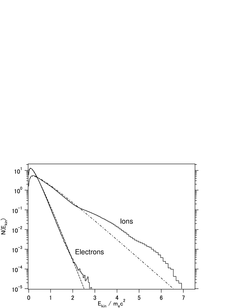
Figure 14.— Kinetic energy distributions of the electrons and the ions measured in the downstream frame (solid histograms) normalized by the electron rest mass energy in the downstream region within $2624\lambda_{\mathrm{e}}<x<2656\lambda_{\mathrm{e}}$. The dashed and dotted curves are the Maxwellian distributions with temperatures of $k_{\mathrm{B}}T_{\mathrm{e}}/m_{\mathrm{e}}c^{2}=0.14$ for electrons and $k_{\mathrm{B}}T_{\mathrm{i}}/m_{\mathrm{e}}c^{2}=0.42$ for ions, respectively.

Using the above results, the shock jump conditions are calculated as follows. In the shock rest frame, the upstream flow velocity $V_{1}$ and the downstream flow velocity $V_{2}$ are given by $V_{1}=0.33c$ and $V_{2}=0.084c$, respectively. Thus, we have $V_{1}/V_{2}\sim 3.9$, $N_{2}/N_{1}\sim 4.1$, and $(k_{\mathrm{B}}(T_{\mathrm{e}}+T_{\mathrm{i}})/m_{\mathrm{i}})^{1/2}\sim 0.14c$, where $N_{1}(=n_{\mathrm{e0}})$ and $N_{2}$ are the number densities in the upstream and downstream regions, respectively. On the other hand, the MHD Rankine–Hugoniot relations (e.g., Tidman & Krall, 1971) give $V_{1}/V_{2}=N_{2}/N_{1}\sim 4$ and $(k_{\mathrm{B}}(T_{\mathrm{e}}+T_{\mathrm{i}})/m_{\mathrm{i}})^{1/2}\sim 0.15c$ in the high Mach number limit. Hence, the simulation results agree very well with the MHD Rankin–Hugoniot relations. Even although, in the downstream region, the magnetic field reaches $\sim 15$ times the upstream fields [see Fig. 3(b)], the plasma beta is still high ($\beta\sim 25$) and the magnetic pressure is negligible for the jump condition.

3.4. Acceleration of reflected ions

As Fig. 14 shows, a fraction of the ions are slightly accelerated to $E_{\mathrm{kin}}/m_{\mathrm{e}}c^{2}\sim 3-6$ (measured in the downstream frame) and form suprathermal populations. Figure 15(a) shows the trajectories of two typical accelerated ions (red and blue curves) together with that of a non-accelerated ion (green curve).

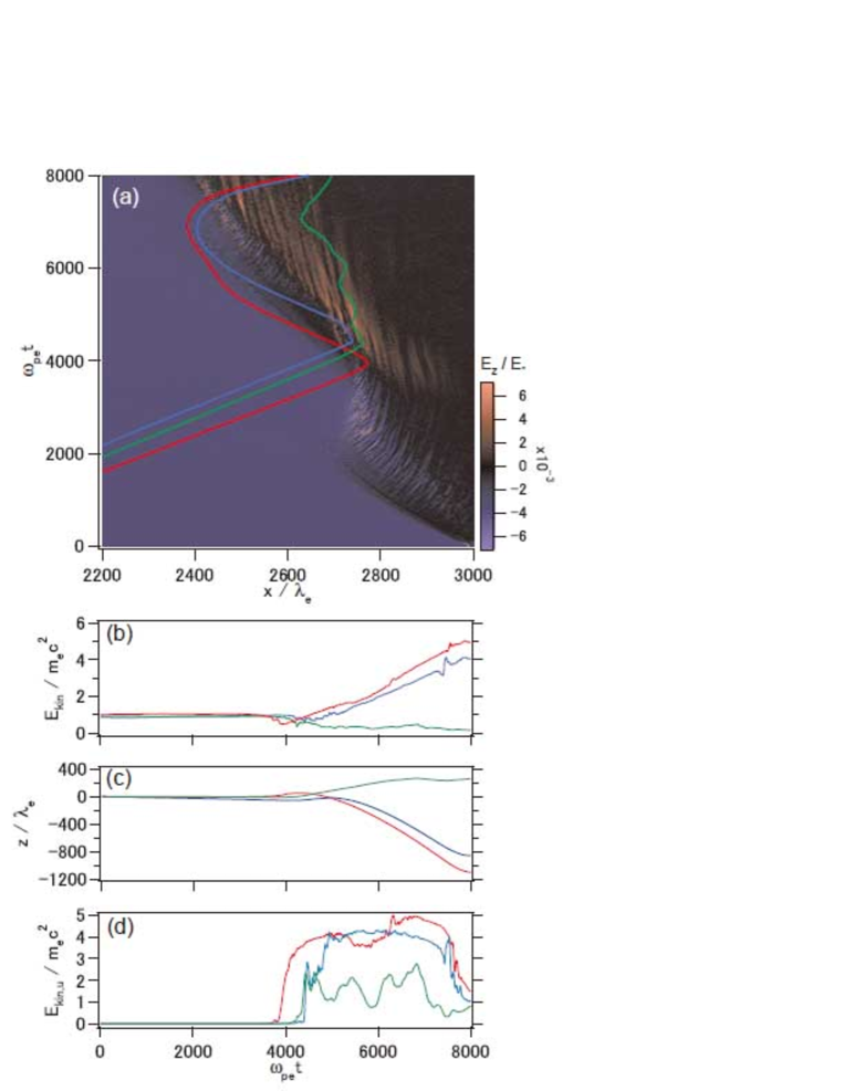
Figure 15.— Histories of two accelerated ions (red and blue curves) and one non-accelerated ion (green curve): (a) Trajectories on the evolution of $E_{z}$. (b) Kinetic energies of the ions measured in the downstream frame. (c) $z$-coordinates of the ions. (d) Kinetic energies of the ions measured in the upstream frame.

It is clear that accelerated ions are reflected at the shock front (i.e., the ramp) and go around the upstream region, whereas non-accelerated ions are directly transmitted downstream. Figure 15(b) shows the kinetic energy history of the three ions measured in the downstream frame. It reveals that the kinetic energies of the ions increase while they are in the upstream region. This is simply acceleration by the motional electric field $E_{z}=-V_{x}B_{y}/c$ in the downstream frame while they are gyrating in the foot region (Auer et al., 1971; Phillips & Robson, 1972) after specular reflection at the shock front (Paschmann et al., 1982; Gosling et al., 1982; Schwartz et al., 1983). As Fig. 15(c) shows, the ions are accelerated when propagating in the $-z$-direction. This process can be understand more clearly in the upstream frame where there is (essentially) only a background magnetic field and no motional electric field. Figure 15(d) shows the same kinetic energy histories as Fig. 15(b) but measured in the upstream frame. It shows that the ions gain energy at the reflection and subsequently their kinetic energy remains almost constant. Thus, the ion acceleration is simply due to reflection at the ramp.

3.5. Currents and magnetic field

Figure 16 shows each component of the current density and the magnetic field. The upstream background field, which is in the $y$ direction, is compressed in the shock transition region as in the 1D simulations, although it fluctuates considerably in the present case. As discussed above, many current filaments exist in the foot region of the shock in $J_{x}$ and $J_{z}$; the filamentary structures observed in the ion number density in Fig. 2 indicate the presence of these current filaments. The filaments generate a magnetic field in the same way as a Weibel-mediated shock in unmagnetized plasmas except that in the present cases $B_{x}$ and $B_{y}$ components are generated by the current filaments in addition to the $B_{z}$ component because the background field deflects the particles in the $z$-direction and the current filaments can have a $J_{z}$ component as well as a $J_{x}$ component.

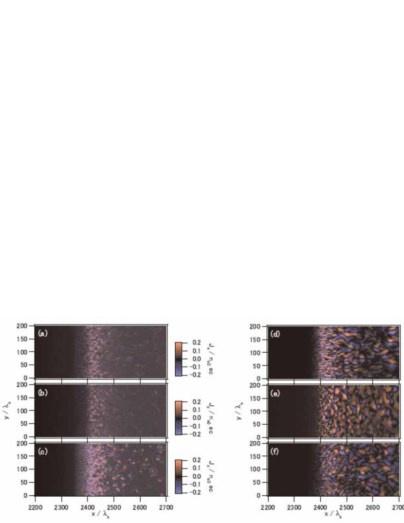
Figure 16.— Left panel: each component of the current density (a) $J_{x}$, (b) $J_{y}$, and (c) $J_{z}$ normalized by $n_{\mathrm{e0}}ec$. Right panel: each component of the magnetic field (d) $B_{x}$, (e) $B_{y}$, and (f) $B_{z}$ normalized by $B_{0}$. There are numerous current filaments in the shock transition region and the downstream region and they generate the magnetic field.

Figure 17 shows the magnetic field strength normalized by the upstream background magnetic field, $|B|/B_{0}$. There are some strong, highly tangled magnetic fields in the transition region ($|B|/B_{0}\sim 40$) and the downstream region ($|B|/B_{0}\sim 15$, which is much larger than the magnetic field strength when merely compressed $\sim 4$).

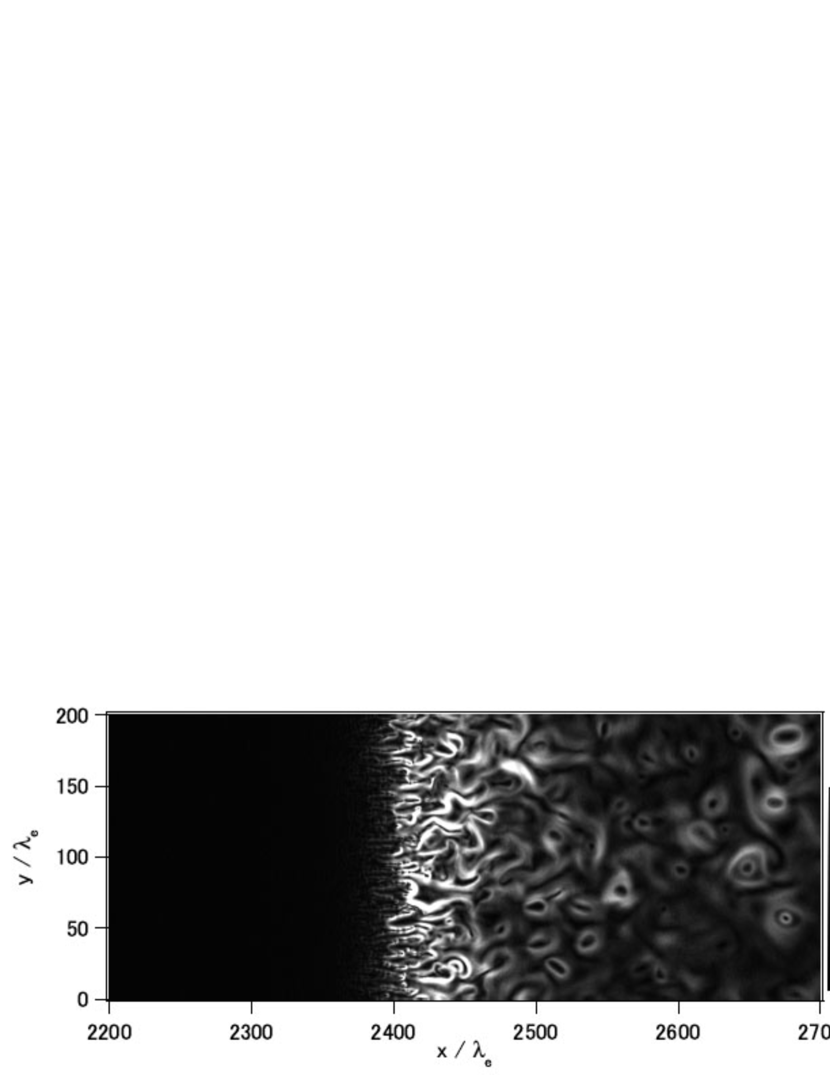
Figure 17.— Magnetic field strength normalized by the upstream background magnetic field, $|B|/B_{0}$. There is a strong, highly tangled magnetic field in both the shock transition region ($|B|/B_{0}\sim 40$) and the downstream region ($|B|/B_{0}\sim 15$).

Figure 18 shows enlargements of the current density in the $z$ direction, $J_{z}$, and the magnetic field strength $|B|$ in a rectangular area in the downstream region ($2550\lambda_{\mathrm{e}}<x<2700\lambda_{\mathrm{e}}$ and $50\lambda_{\mathrm{e}}<y<200\lambda_{\mathrm{e}}$). It is evident that the downstream tangled magnetic field is mainly generated by the current filaments in $J_{z}$. The filaments have typical sizes of $\sim 2-4\lambda_{\mathrm{i}}$, where $\lambda_{\mathrm{i}}\equiv(m_{\mathrm{i}}/m_{\mathrm{e}})^{1/2}\lambda_{\mathrm{e}}$ is the ion inertial length, which is slightly larger than the filament size in the foot region. This can be explained by current filaments coalescing downstream of the foot region. Some of the current filaments have a complex coaxial structure in that they are surrounded by return and anti-return currents.

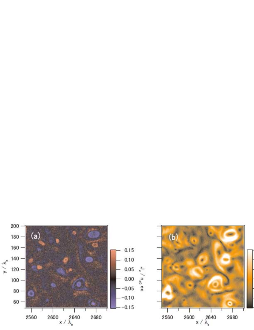
Figure 18.— (a) Current density $J_{z}$ normalized by $n_{\mathrm{e0}}ec$ and (b) magnetic field strength $|B|$ normalized by the upstream field $B_{0}$ in the downstream region $2550\lambda_{\mathrm{e}}<x<2700\lambda_{\mathrm{e}}$ and $50\lambda_{\mathrm{e}}<y<200\lambda_{\mathrm{e}}$. There are numerous current filaments carrying currents in the z-direction and they mainly generate the downstream tangled magnetic field. Some of the current filaments have a coaxial structure.

Coalescence of current filaments that carry a current in the $x$-direction in the foot region is inhibited due to the dimensionality of the simulation, while current filaments in the $z$-direction can merge with each other (c.f. Morse, 1971; Lee & Lampe, 1973; Kato, 2005). Furthermore, the current filaments in the $z$-direction are not affected by instabilities in the current direction, such as the kink instability. Therefore, the current structures in the foot and downstream regions may still differ in three dimensions.

3.6. Early evolution

It is interesting to note the evolution of the system before the effect of the background magnetic field becomes significant (i.e., $t\leq\Omega_{i}^{-1}\sim 2000\omega_{\mathrm{pe}}^{-1}$). In this period, the plasma is effectively unmagnetized and another kind of shock, namely an unmagnetized shock, appears. Figures 19 and 20 respectively show the evolution of the ions in the $x$–$u_{x}$ phase space and that of the ion number density. At a very early time ($\omega_{\mathrm{pe}}t=500$), the incoming ions and the ions reflected by the wall at $x=3000\lambda_{\mathrm{e}}$ form a counterstreaming beam system and the number density in the overlapping region simply becomes twice the upstream number density. The two populations then start to interact ($1000\leq\omega_{\mathrm{pe}}t\leq 2000$) and the density on the right side of the overlapping region increases. As shown below, this interaction is due to the magnetic field generated by the ion beam–Weibel instability in the overlapping region that deflects the ions; this provides a kind of dissipation mechanism. At a later time ($3000\leq\omega_{\mathrm{pe}}t\leq 4000$), the effect of the background magnetic field becomes important and incoming ions start to accumulate around $x\sim 2775\lambda_{\mathrm{e}}$. Most of the ions that are initially reflected by the wall gyrate back downstream due to the background magnetic field by $\omega_{\mathrm{pe}}t=3000$. Instead, at $\omega_{\mathrm{pe}}t=4000$, another reflected ion population appears around $x=2700\lambda_{\mathrm{e}}$; the ions in this population have been newly reflected at the ‘ramp’ ($x\sim 2750\lambda_{\mathrm{e}}$). Thus, the structure changes from an unmagnetized shock to a magnetized one around that time.

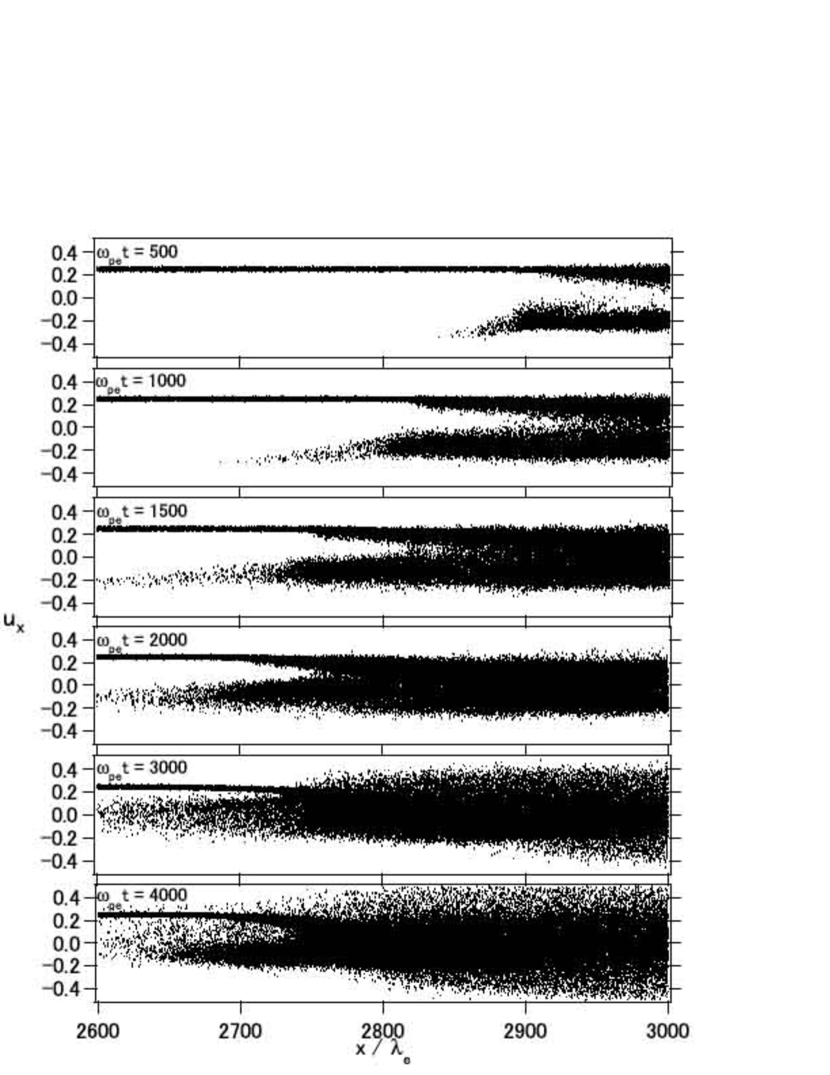
Figure 19.— $x$–$u_{x}$ phase space plots of the ions in the early evolution. Phase space plots at (from top to bottom) $\omega_{\mathrm{pe}}t=500$, $1000$, $1500$, $2000$, $3000$, and $4000$.

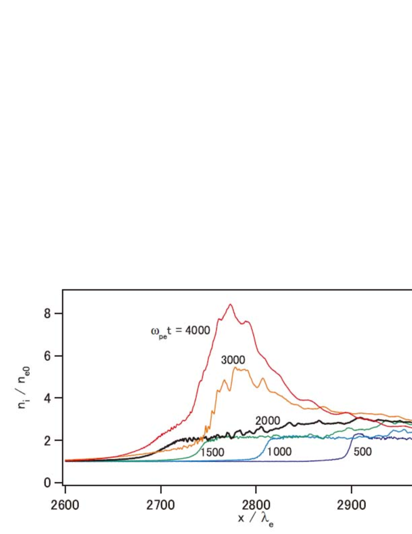
Figure 20.— Time evolution of the ion number density for $\omega_{\mathrm{pe}}t=500$, $1000$, $1500$, $2000$, $3000$, and $4000$.

Figure 21 shows the ion number density, the $x$-component of the current density $J_{x}$, and the $z$-component of the magnetic field $B_{z}$ at $\omega_{\mathrm{pe}}t=2000$. It is evident that many current filaments are generated in the interacting region and generate a strong magnetic field around themselves. A filamentary structure is also observed in the number density corresponding to the current filaments. These current filaments are generated by the ion beam-Weibel instability between the counterstreaming ion populations. The generated magnetic field provides the dissipation mechanism for the ions to form the unmagnetized shock.

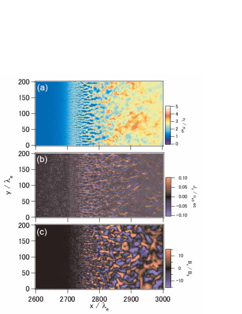
Figure 21.— (a) The ion number density, (b) the $x$-component of the current density, and (c) the $z$-component of the magnetic field at $\omega_{\mathrm{pe}}t=2000$. It is evident that many current filaments exist and generate a strong magnetic field, which eventually isotropizes the incoming ions.

Figure 22 shows $u_{x}$–$u_{y}$ plots in the following three regions: $2700<x/\lambda_{\mathrm{e}}<2800$, $2800<x/\lambda_{\mathrm{e}}<2900$, and $2900<x/\lambda_{\mathrm{e}}<3000$. The ions are almost completely isotropized and form a ring-like distribution in the $u_{x}$-$u_{y}$ plane far downstream ($2900<x/\lambda_{\mathrm{e}}<3000$). Since the beam-Weibel instability generates only the $z$-component of the magnetic field in this 2D configuration, the magnetic field deflects the ions only in the $u_{x}$-$u_{y}$ plane. However, in three dimensions, the generated magnetic field can have the $y$-component and the ions can be deflected in all directions, resulting in three-dimensional dissipation.

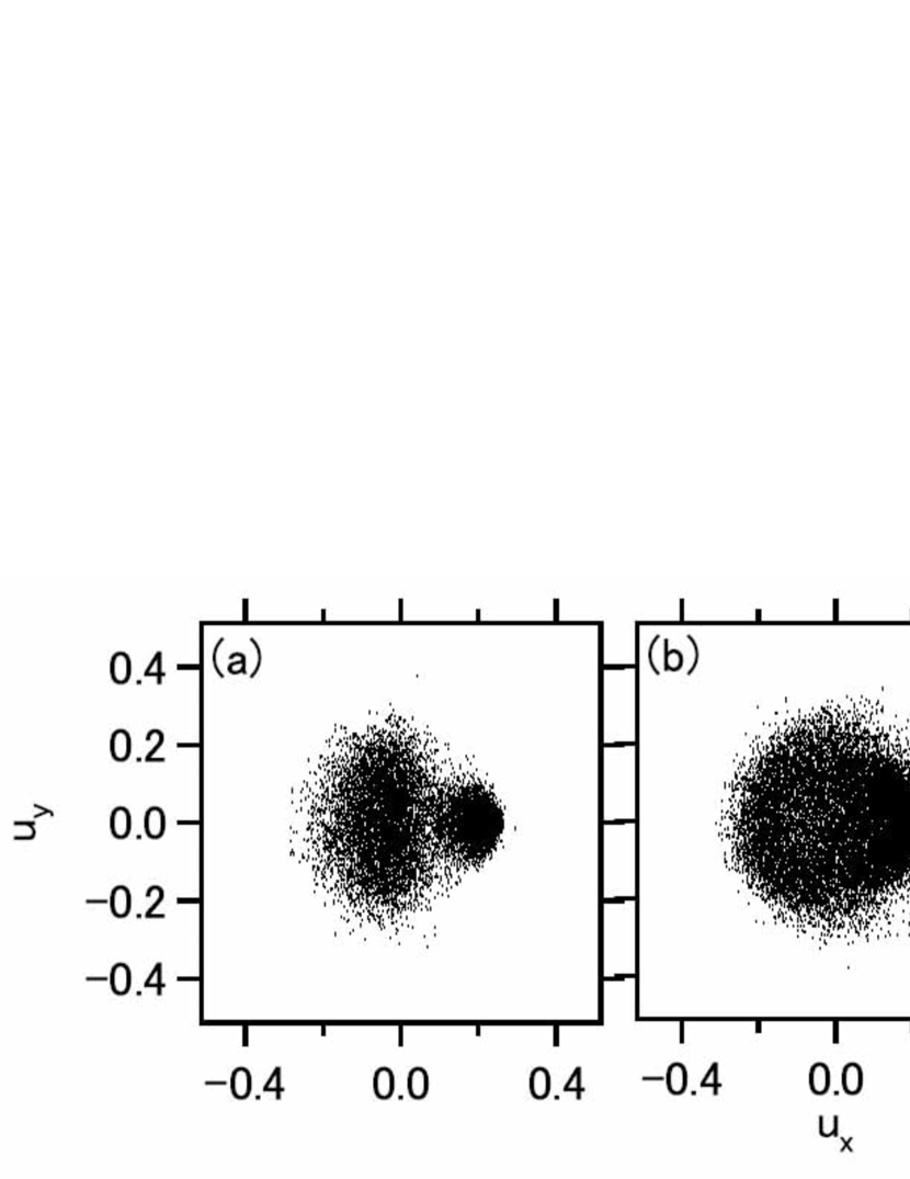
Figure 22.— $u_{x}$ – $u_{y}$ plots of the ions at $\omega_{\mathrm{pe}}t=2000$ in three regions: (a) $2700<x/\lambda_{\mathrm{e}}<2800$, (b) $2800<x/\lambda_{\mathrm{e}}<2900$, and (c) $2900<x/\lambda_{\mathrm{e}}<3000$. In (c), the ions are almost isotropized in the $u_{x}$ – $u_{y}$ plane, forming a ring-like distribution.

The dissipated ions form the downstream region of the shock and the shock structure propagates upstream at an almost constant speed, as shown in Fig. 1 for $1500\leq\omega_{\mathrm{pe}}t\leq 2000$. In the present simulation, this Weibel-mediated shock disappears when the effect of the background magnetic field becomes significant at later times. However, this shock can propagate steadily upstream when there is no background field (Kato & Takabe, 2008).

4. DISCUSSION

In the previous section it was found that the filamentary structures in our simulation are generated by the ion beam–Weibel instability in the foot region. Similar structures have been found in the foot or overshoot region in 2D PIC or hybrid simulations with lower Mach numbers. There are two different causes for these structures: the emission of whistler waves at the ramp (Krauss-Varban et al., 1995; Hellinger et al., 2007; Lembège et al., 2009) and the emission of Alfvén waves due to the Alfvén ion cyclotron instability, resulting in a structure called rippling (Winske & Quest, 1988; Lowe & Burgess, 2003). Since these are associated with waves generated at the ramp or the overshoot and which then propagate upstream, these processes could also be related to the filamentary structures in our simulation. The wavenumber range of the whistler wave is given by (Ichimaru, 1973):

$$\frac{4m_{\mathrm{e}}}{m_{\mathrm{i}}}\ll\frac{n_{\mathrm{e0}}}{n_{\mathrm{e}}}\left(\frac{kc}{\omega_{\mathrm{pe}}}\right)^{2}\ll 1,$$ (20)

where $n_{\mathrm{e}}$ is the local electron number density at which the whistler wave exists and $n_{\mathrm{e0}}$ and $\omega_{\mathrm{pe}}$ are defined for the far upstream. The left-hand side is $\sim 0.133$ in our simulation and if we take $n_{\mathrm{e}}/n_{\mathrm{e0}}\sim 2$ [Fig. 6(c)] and $kc/\omega_{\mathrm{pe}}\sim 1$ [Fig. 12(d)] as typical values, the above condition is (marginally) satisfied. However, if the structure is related with (standing) whistler waves, its group velocity must be greater than the shock speed (in the upstream frame):

$$v_{\mathrm{g}}=\frac{\partial\omega}{\partial k}=2\frac{B}{B_{0}}\left(\frac{n_{\mathrm{e}}}{n_{\mathrm{e0}}}\right)^{-1}\frac{|\omega_{\mathrm{ce}}|}{\omega_{\mathrm{pe}}}\frac{kc^{2}}{\omega_{\mathrm{pe}}}>V_{\mathrm{sh}},$$ (21)

where $B_{0}$ and $\omega_{\mathrm{ce}}$ are defined for the far upstream, whereas $B$ is the local value. [Here, we neglect the dependence of the propagation angle and hence it is just a necessary condition; c.f., Krauss-Varban et al. (1995).] This condition can be rewritten as

$$M_{\mathrm{A}}<2\frac{B}{B_{0}}\left(\frac{n_{\mathrm{e}}}{n_{\mathrm{e0}}}\right)^{-1}\left(\frac{m_{\mathrm{i}}}{m_{\mathrm{e}}}\right)^{1/2}\frac{kc}{\omega_{\mathrm{pe}}}.$$ (22)

In our simulation, the right-hand side is $\sim 10-30$, whereas the left-hand side is $\sim 130$. Thus, the filamentary structure observed in our simulation does not originate from whistler wave emission. On the other hand, the result of the simulation by Lembège et al. (2009) with $m_{\mathrm{i}}/m_{\mathrm{e}}=400$ satisfies this condition if $B/B_{0}\sim n_{\mathrm{e}}/n_{\mathrm{e0}}$; the right-hand side is $\sim 2kc/\omega_{\mathrm{pi}}\sim 14.6$, whereas the left-hand side is $\sim 4.93$. Assuming $kc/\omega_{\mathrm{pe}}\sim 1$ and $B\propto n_{\mathrm{e}}$, a rough condition for the Alfvén Mach number is given by

$$M_{\mathrm{A}}<2(m_{\mathrm{i}}/m_{\mathrm{e}})^{1/2}.$$ (23)

This gives $M_{\mathrm{A}}\leq 11$ for the mass ratio in our simulation ($m_{\mathrm{i}}/m_{\mathrm{e}}=30$) and $M_{\mathrm{A}}\leq 86$ for the real mass ratio of $m_{\mathrm{i}}/m_{\mathrm{e}}=1836$. The rippling (Winske & Quest, 1988; Lowe & Burgess, 2003) cannot be the cause of the filamentary structure in our simulation because (1) the rippling develops in the overshoot region, whereas the filamentary structure in our simulation develops in the foot region; (2) the wavelength observed in our simulation ($\lambda\sim 8\lambda_{\mathrm{e}}$) is smaller than that of Alfvén waves ($\lambda_{A}>3\lambda_{\mathrm{i}}\sim 16\lambda_{\mathrm{e}}$ for $m_{\mathrm{i}}/m_{\mathrm{e}}=30$); and (3) the Alfvén speed in the foot is smaller than the shock speed. Nevertheless, comparison of Fig. 16 with the figures in Winske & Quest (1988) reveals that the structures of the magnetic field and the number density at and behind the overshoot are similar to each other. Therefore, the rippling mechanism may also operate there in our simulation. Lembège et al. (2009) showed that these structures can also be affected by the dimensionality of the simulations in 2D simulations; the structures when the background magnetic field lies in the simulation plane may differ from those when it is perpendicular to the plane.

Electron acceleration was not observed in our simulation, whereas Amano & Hoshino (2009) observed a kind of electron acceleration in a perpendicular shock in their 2D PIC simulation, which used similar parameters to ours. The main reason for this is considered to be the different directions of the upstream background field: in our simulation it lay in the simulation plane, whereas in the simulation by Amano & Hoshino (2009) it was out of the plane. This again demonstrates that dimensionality can affect the results, even for 2D simulations.

The ion–ion streaming instability (Stringer, 1964; Ohnuma & Hatta, 1965; Forslund & Shonk, 1970), which has a wavevector that is highly oblique to the streaming direction, can be driven by the interaction between the incoming ions and the reflected ions streaming upstream in the foot region and it can contribute to ion heating (Auer et al., 1971; Papadopoulos et al., 1971; Wu et al., 1984; Ohira & Takahara, 2008). [This instability can also be driven in front of electrostatic shocks in two dimensions (Kato & Takabe, 2010).] However, this instability was not observed in our simulation (see the right panels in Fig. 11). This is due to the high temperature of the reflected ions streaming upstream, $T_{\mathrm{R-}}$, in our simulation. According to Ohira & Takahara (2008), the ion–ion streaming instability is efficient for wavenumbers $k>k_{\mathrm{De}}$, whereas it is damped for $k>k_{\mathrm{Di}}$ due to the thermal motion of the ions. Therefore, $k_{\mathrm{De}}<k_{\mathrm{Di}}$ is a necessary condition for efficient growth of the instability. In the present case, the two ion populations have different temperatures (Fig. 7) and the Debye wavenumber of the reflected ions, $k_{\mathrm{D,R_{-}}}$, should be used to evaluate the thermal damping effect. Thus, the condition for effective growth of the ion–ion streaming instability is $k_{\mathrm{De}}<k_{\mathrm{D,R_{-}}}$ or

$$\frac{T_{\mathrm{R-}}}{T_{\mathrm{e}}}<\frac{n_{\mathrm{R-}}}{n_{\mathrm{e}}}.$$ (24)

The right-hand side of this equation is always smaller than unity, whereas the left-hand side is larger than unity in our simulation, as shown in Fig. 8. For example, at $x=2375\lambda_{\mathrm{e}}$, the ratios are $T_{\mathrm{R-}}/T_{\mathrm{e}}=4.2$ and $n_{\mathrm{R-}}/n_{\mathrm{e}}=0.32$, respectively (see Table 1). Hence, the above condition is not satisfied and this would explain why the instability does not grow in our simulation. To examine the effect of $T_{\mathrm{R-}}$ more quantitatively, we performed linear analysis with the parameters obtained from the simulation at $\omega_{\mathrm{pe}}t=8000$ and $x=2375\lambda_{\mathrm{e}}$, but changing $T_{\mathrm{R-}}$ in the same way as in Fig. 9. Figure 23 shows the linear growth rates, the wavenumbers, and the angles between the wave vector and the streaming direction of the most unstable mode of the ion–ion streaming instability as functions of $T_{\mathrm{R-}}$. It shows that the instability depends strongly on $T_{\mathrm{R-}}$. In particular, for $T_{\mathrm{R-}}/T_{\mathrm{e}}\geq 0.35$, it does not grow at all. Thus, the temperature of the reflected ions ($T_{\mathrm{R-}}$) is important for growth of the instability in the foot region as well as the Buneman instability.

Figure 23.— (a) The linear growth rate, (b) wavenumber, and (c) angle of the most unstable mode of the ion–ion streaming instability as functions of the temperature of the reflected ions streaming upstream, $T_{\mathrm{R-}}$, with the other parameters obtained from the simulation at $\omega_{\mathrm{pe}}t=8000$ and $x=2375\lambda_{\mathrm{e}}$, as in Fig. 9. The arrow indicates the initial value of $T_{\mathrm{R-}}$ in the simulation. It is clear that the instability significantly depends on $T_{\mathrm{R-}}$.

Finally, we mention the possibility of generating magnetized shocks in experiments. Present large-scale laser facilities can generate collisionless plasma flows at speeds of $\sim 1000$ km s^-1 (Takabe et al., 2008). Thus, if magnetized collisionless plasmas flowing at this velocity can be generated in laboratories, it should be possible to perform experiments on magnetized shocks. Table 2 shows the required background magnetic field strengths $B_{0}$ for several sigma values and for a number density of $n_{\mathrm{e0}}=10^{20}$ cm^-3 together with the corresponding ion gyration time, $T_{g}$, and ion gyro radius, $r_{g}$. In this table, the gyration time and the gyro radius are calculated for an ion mass of $1836m_{\mathrm{e}}$ and a flow velocity of 1000 km s^-1. Sigmas of $\tilde{\sigma}=10^{-3}$ or $\tilde{\sigma}=10^{-4}$ give achievable values for present large-scale laser facilities.

Table 2 Magnetic field strength required for experiments

$\tilde{\sigma}$	$\tilde{M_{\mathrm{A}}}$	$B_{0}$ (G)	$T_{g}$ (s)	$r_{g}$ (m)
$10^{-2}$	$10$	$4.6\times 10^{5}$	$1.4\times 10^{-9}$	$2.3\times 10^{-4}$
$10^{-3}$	$32$	$1.4\times 10^{5}$	$4.7\times 10^{-9}$	$7.3\times 10^{-4}$
$10^{-4}$	$100$	$4.6\times 10^{4}$	$1.4\times 10^{-8}$	$2.3\times 10^{-3}$
$10^{-5}$	$320$	$1.4\times 10^{4}$	$4.7\times 10^{-8}$	$7.3\times 10^{-3}$

5. CONCLUSION

We performed a 2D PIC simulation to investigate collisionless shocks propagating in weakly magnetized electron–ion plasmas at nonrelativistic speeds with a sigma of $\tilde{\sigma}=10^{-4}$. We showed that current filaments are generated within the foot region by the ion beam–Weibel instability and that they generate magnetic fields in the same manner as for Weibel-mediated shocks in unmagnetized plasmas. The magnetic field strength generated by the current filaments is comparable with or even stronger than those of the compressed background magnetic field. Therefore, these filaments and their associated magnetic fields, which cannot be analyzed by 1D simulations, are important in the formation of collisionless shocks in weakly magnetized plasmas. There are current filaments in the downstream region and they generate a tangled magnetic field that is typically 15 times stronger than the upstream background field. The thermal energies of electrons and ions in the downstream region are not in equipartition and their temperature ratio is given by $T_{\mathrm{e}}/T_{\mathrm{i}}\sim 0.33$. We found a fraction of the ions were slightly accelerated on reflection at the shock, whereas significant electron acceleration was not observed in our simulation. The simulation results agree very well with the Rankine–Hugoniot relations. It was also shown that electrons and ions are heated in the foot region by the Buneman instability (for electrons) and the ion-acoustic instability (for both electrons and ions). However, the growth rate of the Buneman instability was significantly reduced from typical growth rates of this instability because of the relatively high temperature of the reflected ions. For the same reason, ion–ion streaming instability did not grow in the foot region.

References

- Acero et al. (2007) Acero, F., Ballet, J., & Decourchelle, A. 2007, A&A, 475, 883
- Amano & Hoshino (2009) Amano, T., & Hoshino, M. 2009, ApJ, 690, 244
- Auer et al. (1971) Auer, P. L., Kilb, R. W., & Crevier, W. F. 1971, J. Geophys. Res., 76, 2927
- Bamba et al. (2003) Bamba, A., Yamazaki, R., Ueno, M., & Koyama, K. 2003, ApJ, 589, 827
- Bell (2004) Bell, A. R. 2004, MNRAS, 353, 550
- Birdsall & Langdon (1991) Birdsall, C. K., & Langdon, A. B. 1991, Plasma Physics via Computer Simulation (IOP Publishing: Bristol).
- Blandford & Eichler (1987) Blandford, R. D. & Eichler, D. 1987, Phys. Rep., 154, 1
- Brainerd (2000) Brainerd, J. J. 2000, ApJ, 538, 628
- Buneman (1958) Buneman, O. 1958, Phys. Rev. Lett., 1, 8
- Burgess (1989) Burgess, D., Wilkinson, W. P., & Schwartz, S. J. 1989, J. Geophys. Res., 94, 8783
- Cargill & Papadopoulos (1988) Cargill, P. J., & Papadopoulos, K. 1988, ApJ, 329, L29
- Chang et al. (2008) Chang, P., Spitkovsky, A., & Arons, J. 2008, ApJ, 674, 378
- Davidson et al. (1972) Davidson, R. C., Hammer, D. A., Haber, I., & Wagner, C. E. 1972, Phys. Fluids, 15, 317
- Dieckmann & Shukla (2006) Dieckmann, M. E., & Shukla, P. K. 2006, Plasma Phys. Control. Fusion, 48, 1515
- Drury (1983) Drury, L. O’C. 1983, Rep. Prog. Phys., 46, 973
- Forslund & Shonk (1970) Forslund, D. W., & Shonk, C. R. 1970, Phys. Rev. Lett., 5, 281
- Fried (1959) Fried, B. D. 1959, Phys. Fluids, 2, 337
- Fried & Conte (1961) Fried, B. D. & Conte, S. D. The plasma dispersion function (Academic Press, New York, 1961).
- Ghavamian et al. (2002) Ghavamian, P., Winkler, P. F., Raymond, J. C., & Long, K. S. 2002, ApJ, 572, 888
- Giacalone & Jokipii (2007) Giacalone, J., & Jokipii, J. R. 2007, ApJ, 663, L41
- Gosling et al. (1982) Gosling, J. T., Thomsen, M. F., Bame, S. J., Feldman, W. C., Paschmann, G., & Sckopke, N. 1982, Geophys. Res. Lett., 9, 1333
- Hellinger et al. (2007) Hellinger, P., Trávníček, P., Lembège, B., & Savoini, P. 2007, Geophys. Res. Lett., 34, L14109
- Hoshino (2001) Hoshino, M. 2001, Prog. Theor. Phys. Suppl., 143, 149
- Hoshino & Shimada (2002) Hoshino, M., & Shimada, N. 2002, ApJ, 572, 880
- Ichimaru (1973) Ichimaru, S. 1973, Basic Principles of Plasma Physics (W. A. Benjamin: Massachusetts).
- Inoue et al. (2009) Inoue, T., Yamazaki, R., & Inutsuka, S. 2009, ApJ, 695, 825
- Kato (2005) Kato, T. N. 2005, Phys. Plasmas, 12, 080705
- Kato (2007) Kato, T. N. 2007, ApJ, 668, 974
- Kato & Takabe (2008) Kato, T. N., & Takabe, H. 2008, ApJ, 681, L93
- Kato & Takabe (2010) Kato, T. N., & Takabe, H. 2010, Phys. Plasmas, 17, 032114
- Kazimura et al. (1998) Kazimura, Y., Sakai, J. I., Neubert, T., & Bulanov, S. V. 1998, ApJ, 498, L183
- Koyama et al. (1995) Koyama, K., Petre, R., Gotthelf, E. V., Hwang, U., Matsuura, M., Ozaki, M., & Holt, S. S. 1995, Nature, 378, 255
- Krauss-Varban et al. (1995) Krauss-Varban, D., Pantellini, F. G. E., & Burgess, D. 1995 Geophys. Res. Lett., 22, 2091
- Landau & Lifshitz (1980) Landau, L. D., & Lifshitz, E. M. 1980, Statistical Physics (3rd ed. part 1; Butter-Heinemann: Oxford).
- Lee & Lampe (1973) Lee, R. and Lampe, M. 1973, Phys. Rev. Lett., 31, 1390
- Lembège et al. (2009) Lembège, B., Savoini, P., Hellinger, P., & Trávníček, P. M. 2009, J. Geophys. Res., 114, A03217
- Leroy (1981) Leroy, M. M., Goodrich, C. C., Winske, D., Wu, C. S., & Papadopoulos, K. 1981, Geophys. Res. Lett., 8, 1269
- Leroy (1983) Leroy, M. M. 1983, Phys. Fluids, 26, 2742
- Long et al. (2003) Long, K. S., Reynolds, S. P., Raymond, J. C., Winkler, P. F., Dyer, K. K., & Petre, R. 2003, ApJ, 586, 1162
- Lowe & Burgess (2003) Lowe, R. E., & Burgess, D. 2003, Ann. Geophys., 21, 671
- McClements et al. (2001) McClements, K. G., Dieckmann, M. E., Ynnerman, A., Chapman, S. C., & Dendy, R. O. 2001, Phys. Rev. Lett., 87, 255002
- Medvedev & Loeb (1999) Medvedev, M. V., & Loeb, A. 1999, ApJ, 526, 697
- Morse (1971) Morse, R. L. & Nielson, C. W. 1971, Phys. Fluids, 14, 830
- Ohira & Takahara (2007) Ohira, Y., & Takahara, F. 2007, ApJ, 661, L171
- Ohira & Takahara (2008) Ohira, Y., & Takahara, F. 2008, ApJ, 688, 320
- Ohnuma & Hatta (1965) Ohnuma, T. & Hatta, Y. 1965 Kakuyugo-Kenkyu, 15, 637
- Papadopoulos et al. (1971) Papadopoulos, K., Davidson, R. C., Dawson, J. M., Haber, I., Hammer, D. A., Krall, N. A., & Shanny, R. 1971, Phys. Fluids, 14, 849
- Papadopoulos (1988) Papadopoulos, K. 1988, Ap&SS, 144, 535
- Paschmann et al. (1982) Paschmann, G., Sckopke, N., Bame, S. J., & Gosling, J. T. 1982, Geophys. Res. Lett., 9, 881
- Phillips & Robson (1972) Phillips, P. E., & Robson, A. E. 1972, Phys. Rev. Lett., 29, 154
- Reynolds et al. (2008) Reynolds, S. P., Borkowski, K. J., Green, D. A., Hwang, U., Harrus, I., & Petre, R. 2008, ApJ, 680, L41
- Schmitz et al. (2002) Schmitz, H., Chapman, S. C., & Dendy, R. O. 2002, ApJ, 570, 637
- Scholer et al. (2003) Scholer, M., Shinohara, I., & Matsukiyo, S. 2003, J. Geophys. Res., 108, 1014
- Schwartz et al. (1983) Schwartz, S. J., Thomsen, M. F., & Gosling, J. T. 1983, J. Geophys. Res., 88, 2039
- Shimada & Hoshino (2000) Shimada, N., & Hoshino, M. 2000, ApJ, 543, L67
- Spitkovsky (2008) Spitkovsky, A. 2008, ApJ, 673, L39
- Stringer (1964) Stringer, T. E. 1964, J. Nucl. Energy Part C, 6, 267
- Takabe et al. (2008) Takabe, H., et al. 2008, Plasma Phys. Control. Fusion, 50, 124057
- Tidman & Krall (1971) Tidman, D. A., & Krall, N. A. 1971, Shock Waves in Collisionless Plasmas (John Wiley & Sons: New York).
- Uchiyama (2007) Uchiyama, Y., Aharonian, F. A., Tanaka, T., Takahashi, T., & Maeda, Y. 2007, Nature, 449, 576
- Umeda et al. (2008) Umeda, T., Yamao, M., & Yamazaki, R. 2008, ApJ, 681, L85
- Vink & Laming (2003) Vink, J., & Laming, J. M. 2003, ApJ, 584, 758
- Völk et al. (2005) Völk, H. J., Berezhko, E. G., & Ksenofontov, L. T. 2005, A&A, 433, 229
- Weibel (1959) Weibel, E. S. 1959, Phys. Rev. Lett., 2, 83
- Winske & Quest (1988) Winske, D., & Quest, K. B. 1988, J. Geophys. Res., 93, 9681
- Wu et al. (1984) Wu, C. S., Winske, D., Zhou, Y. M., Tsai, S. T., Rodriguez, P., Tanaka, M., Papadopoulos, K., Akimoto, K., Lin, C. S., Leroy, M. M., & Goodrich, C. C. 1984, Space Sci. Rev., 37, 63