Multiple Bernoulli series, an Euler-MacLaurin formula, and Wall crossings

Abstract.

Using multiple Bernoulli series, we give a formula in the spirit of Euler-MacLaurin formula. We also give a wall crossing formula and a decomposition formula for multiple Bernoulli series. The study of these series is motivated by formulae of E. Witten for volumes of moduli spaces of flat bundles over a surface.

1. Introduction

Consider a sequence of vectors $\Phi$ lying in a lattice $\Lambda$ of a real vector space $V$. We denote the dual lattice of $\Lambda$ by $\Gamma$. Let $\Gamma_{{\mathrm{reg}}}(\Phi)=\{\gamma\in\Gamma|\;{\langle}\phi,\gamma{\rangle}\neq 0,\;\mbox{for all}\;\phi\in\Phi\}$ be the set of regular elements in $\Gamma$. Let $Z$ be the fundamental domain in $V$ for $\Lambda$ and $dv$ the Lebesgue measure giving measure $1$ to $Z$. Here in introduction we freely identify distributions and generalized functions via this choice of $dv$.

In this paper we study the distribution $\mathcal{B}(\Phi,\Lambda)$ on the torus $V/\Lambda$ defined via its Fourier coefficients as:

$$\int_{Z}\mathcal{B}(\Phi,\Lambda)(v)e^{-{\langle}2i\pi v,\gamma{\rangle}}dv=\begin{cases}\frac{1}{\prod_{\phi\in\Phi}{\langle}2i\pi\phi,\gamma{\rangle}}&\text{if $\gamma\in\Gamma_{{\mathrm{reg}}}(\Phi)$,}\\ 0&\text{otherwise.}\end{cases}$$

We have

$$\mathcal{B}(\Phi,\Lambda)(v)=\sum_{\gamma\in\Gamma_{{\mathrm{reg}}}(\Phi)}\frac{e^{{\langle}2i\pi v,\gamma{\rangle}}}{\prod_{\phi\in\Phi}{\langle}2i\pi\phi,\gamma{\rangle}}.$$

This sum, if not absolutely convergent, has meaning as a distribution.

We call $\mathcal{B}(\Phi,\Lambda)$ the multiple Bernoulli series associated to $\Phi$ and $\Lambda$. They are natural generalizations of Bernoulli series: for $\Lambda={\mathbb{Z}}\omega$ and $\Phi_{k}=[\omega,\omega,\ldots,\omega]$, where $\omega$ is repeated $k$ times with $k>0$, the distribution

$$\mathcal{B}(\Phi_{k},\Lambda)(t\omega)=\sum_{n\neq 0}\frac{e^{2i\pi nt}}{(2i\pi n)^{k}}$$

is equal to $-\frac{1}{k!}B(k,t-[t])$ where $B(k,t)$ denotes the $k^{\text{th}}$ Bernoulli polynomial in variable $t$.

Multiple Bernoulli series appeared in the work of E. Witten in the special case where the sequence $\Phi$ is comprised of positive coroots of a compact connected Lie group $G$ with multiplicity $2g-1$ and $\Lambda$ is the coroot lattice of $G$. Witten shows that ([17], §3) for the above instance of $\Phi$ and $\Lambda$ and for a regular element $v\in Z$, the value of $\mathcal{B}(\Phi,\Lambda)(v)$ is (upto a scalar depending on $G$ and $g$) the symplectic volume of the moduli space $\mathcal{M}(G,g,v)$ of flat $G$-connections on Riemann surface of genus $g$ with one boundary component, around which the holonomy is determined by $v$.

For example, consider $G=\text{SU}(3)$, denote its simple roots by $\{\alpha_{1},\alpha_{2}\}$ and associated coroots by $\{H_{\alpha_{1}},H_{\alpha_{2}}\}$. Then on a Riemann surface of genus $g=2$, the symplectic volume of the moduli space of flat $\text{SU}(3)$-connections with one boundary component marked by $v=a_{1}H_{\alpha_{1}}+a_{2}H_{\alpha_{2}}$ (lying in the fundamental alcove) is given by the following sum

$$\sum_{\begin{subarray}{c}n_{1}\in{\mathbb{Z}},\,n_{2}\in{\mathbb{Z}}\\ n_{1}\neq 0,\,n_{2}\neq 0,\,n_{1}+n_{2}\neq 0\end{subarray}}\frac{e^{2i\pi(n_{1}a_{1}+n_{2}a_{2})}}{(2i\pi n_{1})^{3}(2i\pi n_{2})^{3}(2i\pi(n_{1}+n_{2}))^{3}}$$

up to a scalar multiple.

These series have been extensively studied by A. Szenes ([12],[13]), who gave multidimensional residue formulae for them.

If $f$ is a function on the real line, smooth and sufficiently decreasing, also with sufficiently decreasing derivatives, then the Euler-MacLaurin formula gives

$$\sum_{n\in{\mathbb{Z}}}f(n)=\int_{{\mathbb{R}}}f(t)dt+(-1)^{k-1}\frac{1}{k!}\int_{{\mathbb{R}}}B(k,t-[t])f^{[k]}(t)dt$$

where $f^{[k]}$ denotes the $k^{\text{th}}$ derivative of $f$.

We give a natural generalization of this formula involving $\mathcal{B}(\Phi,\Lambda)$ in Theorem 6.1. The difference between the discrete sum $\sum_{\lambda\in\Lambda}f(\lambda)$ and the integral of $f$ over $V$ will only involve derivatives $(\prod_{\phi\in Y}\partial_{\phi})f$ over ‘long subsets’ $Y$ of $\Phi$, that is, subsets $Y$ such that their complement in $\Phi$ do not span the vector space $V$.

We start with giving some properties of the distribution $\mathcal{B}(\Phi,\Lambda)$ that are pertinent for what follows.

The distribution $\mathcal{B}(\Phi,\Lambda)$ is periodic with respect to $\Lambda$. Moreover, it satisfies a certain recurrence relation which we outline next.

We will call a set with multiplicities a list. Suppose $\Phi$ contains $\phi$ with multiplicity $m$, then we denote the list that contains $\phi$ with multiplicity $m-1$ by $\Phi-\{\phi\}$; whereas we denote the list where all copies of $\phi$ are removed by $\Phi\setminus\{\phi\}$. More generally, for a subset $B$ of $V$, by $\Phi\setminus B$ we mean the list of elements of $\Phi$ not lying in $B$. By $\Phi\cap B$ we mean the list of elements of $\Phi$ lying in $B$.

For an element $\phi$ in $\Phi$, we associate two lists of vectors as follows: First, we consider the list $\Phi-\{\phi\}$ in $V$, and respectively the distribution $\mathcal{B}(\Phi-\{\phi\},\Lambda)$ on $V$. Let $V_{0}:=V/{\mathbb{R}}\phi$ and let $\Lambda_{0}$ denote the image of the lattice $\Lambda$ in $V_{0}$. Secondly, we consider the list $\Phi_{0}$ of elements of $V_{0}$ consisting of the images of the elements in $\Phi-\{\phi\}$. Then we may consider $\mathcal{B}(\Phi_{0},\Lambda_{0})$ as a distribution on $V$ ‘constant in the direction of $\phi$’. Observe that if $\Phi$ contains more than one copy of $\phi$ then $\Phi_{0}$ contains the zero vector and consequently $\mathcal{B}(\Phi_{0},\Lambda_{0})$ is identically zero.

It is clear that the distribution $\mathcal{B}(\Phi,\Lambda)$ satisfies the following recurrence relation

(1.0.1) $$\partial_{\phi}\mathcal{B}(\Phi,\Lambda)=\mathcal{B}(\Phi-\{\phi\},\Lambda)-\mathcal{B}(\Phi_{0},\Lambda_{0}).$$

Assuming that $\Phi=[\phi_{1},\phi_{2},\ldots,\phi_{N}]$ spans a pointed cone, we may define the tempered distribution $T(\Phi)$ defined on test functions $f$ by:

(1.0.2) $$\langle T(\Phi)\,|\,f\rangle=\int_{0}^{\infty}\cdots\int_{0}^{\infty}f(\sum_{i=1}^{N}t_{i}\phi_{i})dt_{1}\cdots dt_{N}.$$

In other words, $T([\phi])$ is the Heaviside distribution ${\langle}H(\phi),f{\rangle}=\int_{0}^{\infty}f(t\phi)dt$ and $T(\Phi)$ is the convolution product

$$H(\phi_{1})*H(\phi_{2})*\cdots*H(\phi_{N})$$

of the Heaviside distributions $H(\phi_{k})$.

If $\Phi$ generates $V$, $T(\Phi)$ is a positive measure on $V$ given by integration against a piecewise polynomial function called a multispline. For any $\phi\in\Phi$,

(1.0.3) $$\partial_{\phi}T(\Phi)=T(\Phi-\{\phi\}).$$

We remark the similarity between the recurrence relations (1.0.1) and (1.0.3). In fact we will express $\mathcal{B}(\Phi,\Lambda)$ in terms of superposition of multispline functions in Theorem 9.3.

If $\Phi$ generates $V$, then the periodic function $\mathcal{B}(\Phi,\Lambda)$ is piecewise polynomial; this we reprove in Section 5.

In the rest of the introduction, for simplicity, we assume that $\Phi$ generates $V$. We call a connected component of the complement of affine walls (that is, hyperplanes that are generated by some elements of $\Phi$ and their translates with respect to the lattice $\Lambda$) in $V$ a tope. For example, Figure 1 depicts topes associated to the system $\Phi=[e_{1},e_{2},e_{1}+e_{2}]$ and $\Lambda={\mathbb{Z}}e_{1}\oplus{\mathbb{Z}}e_{2}$.

Figure 1. ${\mathcal{T}}([e_{1},e_{2},e_{1}+e_{2}],{\mathbb{Z}}e_{1}\oplus{\mathbb{Z}}e_{2})$

Given a tope $\tau$ associated to the system $(\Phi,\Lambda)$, we denote by $\operatorname{Ber}(\Phi,\Lambda,\tau)$ the polynomial function on $V$ such that the restriction of $\mathcal{B}(\Phi,\Lambda)$ to $\tau$ coincides with the restriction of $\operatorname{Ber}(\Phi,\Lambda,\tau)(v)$ to $\tau$.

Let $W$ be an hyperplane in $V$ spanned by some elements of $\Phi$, and let $E\in\Gamma$ be an equation of this hyperplane. We reverse the directions of ‘half of’ the $\phi_{i}$ in $\Phi\setminus W$ in order that they all lie in the strict half space determined by $E$, and define

$$T(\Phi\setminus W,E):=\displaystyle\prod_{\langle\phi_{i},E\rangle<0}-H(-\phi_{i})*\prod_{\langle\phi_{i},E\rangle>0}H(\phi_{i}).$$

$T(\Phi\setminus W,E)$ is a distribution supported on $E\geq 0$. We similarly define $T(\Phi\setminus W,-E)$.

Now we compare the polynomials $\operatorname{Ber}(\Phi,\Lambda,\tau)$ associated to two adjacent topes separated by an hyperplane $W$ (cf. Section 7). The jump can be expressed in terms of a lower dimensional multiple Bernoulli series and a multispline function. More explicitly, we have the following wall crossing formula:

Theorem 1.1.

Let $\tau_{1}$ and $\tau_{2}$ be two adjacent topes separated by the hyperplane $W$ defined by $E$ with $\langle v,E\rangle>0$ for any $v\in\tau_{1}$. Denote by $\tau_{12}$ the tope with respect to the system $(\Phi\cap W,\Lambda\cap W)$ containing $\overline{\tau_{1}}\cap\overline{\tau_{2}}$ in its closure. Let $\operatorname{Ber}^{\tau_{12}}:=\operatorname{Ber}(\Phi\cap W,\Lambda\cap W,\tau_{12})dh$ be the polynomial density on $W$ determined by $\tau_{12}$. Then,

$$(\operatorname{Ber}(\Phi,\Lambda,\tau_{1})-\operatorname{Ber}(\Phi,\Lambda,\tau_{2}))dv=\operatorname{Ber}^{\tau_{12}}*T(\Phi\setminus W,E)-\operatorname{Ber}^{\tau_{12}}*T(\Phi\setminus W,-E).$$

The left hand side of the above equation is a polynomial density; it is easily proven that the right hand side is also a polynomial density.

The wall crossing formula given in the above theorem is analogous to the formula in Boysal-Vergne [1]. This formula is also similar to wall crossing formulae in Hamiltonian geometry for the push-forward of the Liouville measure; indeed, when crossing a wall, this piecewise polynomial measure changes according to the same scheme [9], [7]. Our wall crossing formula in Theorem 1.1 is thus in accordance with the fact that for special cases $\mathcal{B}(\Phi,\Lambda)$ computes the volume of the moduli spaces ${\mathcal{M}}(G,g,v)$. These spaces can be described as symplectic reduction at $v$ of the Jeffrey-Kirwan extended moduli space $M(G,g)$, so that their volume at $v$ is given by the push-forward of the Liouville measure on $M(G,g)$, a piecewise polynomial function periodic with respect to a lattice $\Lambda$. Recall that Jeffrey-Kirwan ([8]) proved wall crossing formulae for integrals on moduli spaces $\mathcal{M}(G,g,v)$, and used them in a fundamental way to compute intersection pairings on $\mathcal{M}(G,g,v)$ when $G=SU(n)$. However, in the general situation that we are considering here, we do not have such a geometric interpretation of the multiple Bernoulli series.

In Section 8 we generalize the above results to the case of affine arrangements.

In Section 9, we give a decomposition formula for $\mathcal{B}(\Phi,\Lambda)$, describing it as a superposition of ‘basic pieces’ made of convolution products of lower dimensional Bernoulli series and multisplines. More precisely, we say that $\mathfrak{s}$ is an admissible subspace of $V$ if $\mathfrak{s}$ is spanned by some elements of $\Phi$, and we say that $\mathfrak{a}$ is affine admissible, if $\mathfrak{a}$ is a translate by $\Lambda$ of an admissible subspace. Given a tope $\tau$, we express the difference between the piecewise polynomial density $\mathcal{B}(\Phi,\Lambda)$ and the polynomial density $\operatorname{Ber}(\Phi,\Lambda,\tau)$ as a sum of distributions $\mathcal{A}(\Phi,\Lambda,\mathfrak{a},\beta)$ associated to proper affine admissible subspaces $\mathfrak{a}$ and the choice of an element $\beta\in\tau$. The supports of these distributions do not intersect $\tau$ and are convolution products of polynomial distributions supported on $\mathfrak{a}$ with multisplines distributions directed towards the exterior of $\tau$. Our construction is inspired by the stratification of a Hamiltonian manifold $M$ using the square of the moment map as Morse function, and we will use a scalar product on $V$. Our decomposition formula is very similar to Paradan’s decomposition of the equivariant index of a twisted Dirac operator on $M$ [11]. In [15], Paradan’s decomposition was proved by combinatorial methods, and used to give a proof that quantization commutes with reduction for compact Hamiltonian manifolds. We follow here very closely the line of approach of [15]. However our superposition is an infinite (but locally finite) superposition. This is in accordance with the fact that for some special cases, our distributions are related to Liouville measures of noncompact Hamiltonian manifolds such as $M(G,g)$ with infinite number of critical components for the square of the moment map.

For example, the periodic polynomial $-B(2,t-[t])/2$ in Figure 2(a) is decomposed in Figure 2(b) as a superposition of a polynomial density with an infinite number of spline functions.

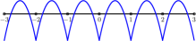
(a)                                               (b)

Figure 2. The decomposition of $\mathcal{B}(\Phi_{2},\Lambda)(t\omega)$.

Acknowledgements

We thank Michel Duflo for various suggestions. The first author wishes to thank École Polytechnique (Palaiseau, France), and the second author wishes to thank Boḡaziçi Üniversitesi (Turkey) for financial support of research visits. The first author is partially supported by Boḡaziçi Üniversitesi (B.U.) Research Fund $5076.$

List of Notations

$$\begin{array}[]{ll}V_{\mathbb{Q}}&\mbox{r-dimensional vector space over ${\mathbb{Q}}$.}\\ V&\mbox{the r-dimensional real vector space $V_{\mathbb{Q}}\bigotimes_{\mathbb{Q}}{\mathbb{R}}$; $v\in V$.}\\ U&\mbox{the dual of $V$; $x\in U$.}\\ {\langle}\;,\;{\rangle}&\mbox{the pairing between $U$ and $V$.}\\ \Gamma&\mbox{a lattice in $U$; $\gamma\in\Gamma$.}\\ \Lambda:=\Gamma^{*}&\mbox{dual lattice in $V$; ${\langle}\Gamma,\Lambda{\rangle}\subset{\mathbb{Z}}$, $\lambda\in\Lambda$.}\\ \Phi&\mbox{a sequence of vectors in $V_{\mathbb{Q}}$; $\phi\in\Phi$.}\\ \mathcal{B}(\Phi,\Lambda)&\mbox{multiple Bernoulli series associated to $\Phi$ and $\Lambda$ (equation \ref{mbseriess}).}\\ B(k,t)&\mbox{$k^{th}$ Bernoulli polynomial.}\\ \mathcal{T}(\Phi,\Lambda)&\mbox{the set of topes associated to the system $(\Phi,\Lambda)$; $\tau$ a tope.}\\ T(X)&\mbox{multivariate spline distribution defined for a set of vectors $X$ in $V$.}\\ \mathcal{R}&\mbox{set of $\Phi$-admissible subspaces of $V$.}\\ W&\mbox{$\Phi$-admissible hyperplane.}\\ H_{\phi}&\mbox{hyperplane in $U$ comprising of vectors $u$ satisfying ${\langle}u,\phi{\rangle}=0$.}\\ \mathcal{H}=\mathcal{H}(\Phi)&\mbox{hyperplane arrangement associated to $\Phi$.}\\ \mathcal{R}_{\mathcal{H}}&\mbox{ring of rational functions on $U$ with poles along $\mathcal{H}$.}\\ \mathcal{G}_{\mathcal{H}}&\mbox{a subspace of $\mathcal{R}_{\mathcal{H}}$ defined in \ref{defgphi}.}\\ \end{array}$$

2. Multiple Bernoulli series and hyperplane arrangements

Let $V_{\mathbb{Q}}$ be an r-dimensional vector space over ${\mathbb{Q}}$, and let $V$ be the real vector space $V_{\mathbb{Q}}\bigotimes_{\mathbb{Q}}{\mathbb{R}}$. Let $U$ denote the dual vector space to $V$. Let $\Lambda$ be a lattice in $V$ contained in $V_{\mathbb{Q}}$ and $\Gamma\subset U$ be the dual lattice to $\Lambda$ so that ${\langle}\Gamma,\Lambda{\rangle}\subset{\mathbb{Z}}$. For a subset $S$ of $V$, we denote by $<S>$ the subspace of $V$ generated by $S$.

Let $Z$ denote the fundamental domain in $V$ for $\Lambda$. Let $d_{\Lambda}v$ be the Lebesgue measure on $V$ giving measure $1$ to $Z$. Our main object of study is certain piecewise polynomial densities on $V$. For our purposes it will be convenient to use the language of distributions. If $f$ is a locally $L^{1}$ function on $V$, or more generally a generalized function, then $f(v)d_{\Lambda}v$ is a distribution on $V$. We use the notation $f(v)d_{\Lambda}v$, although the value of $f$ at the point $v\in V$ has usually no meaning.

For $v_{0}\in V$, the translation ${\rm t}(v_{0})$ acts on distributions on $V$. If $D=f(v)d_{\Lambda}v$, then ${\rm t}(v_{0})D=f(v+v_{0})d_{\Lambda}v$. We identify a distribution $D$ on $V$ periodic with respect to $\Lambda$ (that is ${\rm t}(\lambda)D=D$ for any $\lambda\in\Lambda$) to a distribution $D$ on the torus $V/\Lambda$.

We will say that a locally $L^{1}$ function $f$ is piecewise polynomial, if there exists a decomposition of $V$ in a union of polyhedral pieces $C_{i}$ such that the restriction of $f$ to $C_{i}$ is given by a polynomial formula. We then say that the distribution $f(v)d_{\Lambda}v$ is piecewise polynomial.

If $v\in V$, we denote by $\delta_{v}$ the $\delta$ distribution at $v$: $\langle\delta_{v},f\rangle=f(v)$. The Poisson formula reads as the following equality of distributions

(2.0.1) $$\sum_{\lambda\in\Lambda}\delta_{\lambda}=\sum_{\gamma\in\Gamma}e^{2i\pi\langle\gamma,v\rangle}d_{\Lambda}v.$$

We now introduce the main object of study of this article.

Let $\Phi$ be a sequence of vectors in $V_{\mathbb{Q}}$. Let

$$U_{{\mathrm{reg}}}(\Phi)=\{u\in U|\;{\langle}\phi,u{\rangle}\neq 0,\;\mbox{for all}\;\phi\in\Phi\}.$$

We will denote $\Gamma\cap U_{{\mathrm{reg}}}(\Phi)$ by $\Gamma_{{\mathrm{reg}}}(\Phi)$. Consider the distribution $\mathcal{B}(\Phi,\Lambda)$ on $V/\Lambda$ defined via its Fourier coefficients:

(2.0.2) $$\int_{Z}\mathcal{B}(\Phi,\Lambda)(v)e^{-{\langle}2i\pi v,\gamma{\rangle}}=\begin{cases}\frac{1}{\prod_{\phi\in\Phi}{\langle}2i\pi\phi,\gamma{\rangle}}&\text{if $\gamma\in\Gamma_{{\mathrm{reg}}}(\Phi)$,}\\ 0&\text{otherwise.}\end{cases}$$

We then have

(2.0.3) $$\mathcal{B}(\Phi,\Lambda)=\sum_{\gamma\in\Gamma_{{\mathrm{reg}}}(\Phi)}\frac{e^{{\langle}2i\pi v,\gamma{\rangle}}}{\prod_{\phi\in\Phi}{\langle}2i\pi\phi,\gamma{\rangle}}d_{\Lambda}v.$$

The above sum, if not absolutely convergent, is defined as a distribution. We call $\mathcal{B}(\Phi,\Lambda)$ the multiple Bernoulli series associated to $\Phi$ and $\Lambda$. Clearly, it does not depend on the order of the elements $\phi$ in the sequence $\Phi$ (it only depends on $\Phi$ as a multiset).

Remark 2.1.

The formula (2.0.2) for the Fourier coefficients of $\mathcal{B}(\Phi,\Lambda)$ is very similar to the formula for the Fourier transform of the multispline distribution $T(\Phi)$ (defined in (1.0.2)) on $V$: if $\Phi$ spans a pointed cone, then the Fourier transform of $T(\Phi)$ is a generalized function on $U$ satisfying

$$\int_{V}T(\Phi)(v)e^{-{\langle}2i\pi v,x{\rangle}}=\frac{1}{\prod_{\phi\in\Phi}{\langle}2i\pi\phi,x{\rangle}}$$

on the open set of $U$ given by $\prod_{\phi\in\Phi}{\langle}\phi,x{\rangle}\neq 0$.

We now list some properties of the distribution $\mathcal{B}(\Phi,\Lambda)$:

$\bullet$ If $\Phi$ is the empty set, then

$$\mathcal{B}(\Phi,\Lambda)=\sum_{\gamma\in\Gamma}e^{2i\pi\langle\gamma,v\rangle}d_{\Lambda}v=\sum_{\lambda\in\Lambda}\delta_{\lambda}$$

is the $\delta$-distribution of the lattice $\Lambda$.

$\bullet$ If $\Phi$ contains the zero vector, then $\mathcal{B}(\Phi,\Lambda)$ is identically equal to zero.

$\bullet$ $\mathcal{B}(\Phi,\Lambda)$ is periodic with respect to $\Lambda.$

$\bullet$ Let $\Lambda_{1}\subset\Lambda_{2}$. Then $\mathcal{B}(\Phi,\Lambda_{2})$ is obtained from $\mathcal{B}(\Phi,\Lambda_{1})$ by averaging over $\Lambda_{2}/\Lambda_{1}$:

(2.1.1) $$\mathcal{B}(\Phi,\Lambda_{2})=\sum_{\lambda_{2}\in\Lambda_{2}/\Lambda_{1}}{\rm t}(\lambda_{2})\mathcal{B}(\Phi,\Lambda_{1}).$$

The above relation follows from the fact that, if $\gamma\in\Gamma_{1}\setminus\Gamma_{2}$, then $\sum_{\lambda_{2}\in\Lambda_{2}/\Lambda_{1}}e^{2i\pi{\langle}\gamma,\lambda_{2}{\rangle}}=0.$

$\bullet$ The distribution $\mathcal{B}(\Phi,\Lambda)$ is supported on $<\Phi>+\Lambda$.

Indeed, it is immediate to verify that $(1-e^{{\langle}2i\pi v,\nu{\rangle}})\mathcal{B}(\Phi,\Lambda)=0$ for all $\nu\in\Gamma\cap<\Phi>^{\perp}$.

$\bullet$ If $\Phi$ generates $V$, then $\mathcal{B}(\Phi,\Lambda)$ is piecewise polynomial. We will give a proof of this property in Section 5.

When the lattice $\Lambda$ is fixed, we often use the measure $d_{\Lambda}v$ to identify distributions and generalized functions.

Example 2.2.

Let $\Lambda={\mathbb{Z}}\omega$, and let $\Phi_{k}=[\omega,\omega,\ldots,\omega]$ where $\omega$ is repeated $k$ times. If $k=0$, then $\mathcal{B}(\Phi_{k},\Lambda)(t\omega)=\sum_{n\in{\mathbb{Z}}}e^{2i\pi nt}dt$ is the $\delta$-distribution of the lattice $\Lambda$ by Poisson formula. If $k>0$, then

$$\mathcal{B}(\Phi_{k},\Lambda)(t\omega)=\sum_{n\neq 0}\frac{e^{2i\pi nt}}{(2i\pi n)^{k}}dt=-\frac{1}{k!}B(k,t-[t])dt,$$

where $B(k,t)$ denotes the $k^{\text{th}}$ Bernoulli polynomial in variable $t$ and $[t]$ is the integer part of $t$. (Our normalization for the Bernoulli polynomial is that of Maple). In particular, for $k=1$, we have $\mathcal{B}(\Phi_{1},\Lambda)(t\omega)dt=(\frac{1}{2}-t+[t])dt$ (see Figure 3).

Figure 3. Graph of the function $\mathcal{B}(\Phi_{1},\Lambda)(t\omega)=(\frac{1}{2}-t+[t]$)

If $k>1$, the above series is absolutely convergent and $\mathcal{B}(\Phi_{k},\Lambda)(t\omega)$ is given by integration against a continuous function on ${\mathbb{R}}$.

Example 2.3.

Let $V={\mathbb{R}}e_{1}\oplus{\mathbb{R}}e_{2}$ with lattice $\Lambda={\mathbb{Z}}e_{1}\oplus{\mathbb{Z}}e_{2}$. Let $\Phi=[e_{1},e_{2},e_{1}+e_{2}]$. We write $v\in V$ as $v=v_{1}e_{1}+v_{2}e_{2}$.

We compute the series $\mathcal{B}(\Phi,\Lambda)=\mathcal{B}(v_{1},v_{2})dv_{1}dv_{2}$ where

$$\begin{array}[]{ll}\mathcal{B}(v_{1},v_{2})&=\displaystyle\sum_{\begin{subarray}{c}n_{1}\in{\mathbb{Z}},\,n_{2}\in{\mathbb{Z}}\\ n_{1}\neq 0,\,n_{2}\neq 0,\,n_{1}+n_{2}\neq 0\end{subarray}}\frac{e^{2i\pi(n_{1}v_{1}+n_{2}v_{2})}}{(2i\pi n_{1})(2i\pi n_{2})(2i\pi(n_{1}+n_{2}))}.\end{array}$$

The distribution $\mathcal{B}(\Phi,\Lambda)$ is piecewise polynomial and periodic with respect to $\Lambda={\mathbb{Z}}e_{1}+{\mathbb{Z}}e_{2}$. It is thus sufficient to write the formulae of $\mathcal{B}(v_{1},v_{2})$ for $0<v_{1}<1$ and $0<v_{2}<1$ (see Figure 4).

Figure 4. ${\mathcal{T}}([e_{1},e_{2},e_{1}+e_{2}],{\mathbb{Z}}e_{1}\oplus{\mathbb{Z}}e_{2})$

$$\mathcal{B}(v_{1},v_{2})=\left\{\begin{array}[]{cl}-\frac{1}{6}(1+v_{1}-2v_{2})(v_{1}-1+v_{2})(2v_{1}-v_{2}),&\text{if}\;v_{1}<v_{2}\\ -\frac{1}{6}(v_{1}-2v_{2})(v_{1}-1+v_{2})(2v_{1}-1-v_{2}),&\text{if}\;v_{1}>v_{2}.\end{array}\right.$$

We remark that $3\mathcal{B}(v_{1},v_{2})$ is the symplectic volume of the moduli space of flat $\text{SU}(3)$-connections on a topological torus with one marked point $v=v_{1}H_{\alpha_{1}}+v_{2}H_{\alpha_{2}}$ where $H_{\alpha_{1}}$ and $H_{\alpha_{2}}$ denote coroots associated to simple roots $\{\alpha_{1},\alpha_{2}\}$ of $\text{SU}(3)$.

Example 2.4.

Let $V={\mathbb{R}}e_{1}\oplus{\mathbb{R}}e_{2}$ with lattice $\Lambda={\mathbb{Z}}e_{1}\oplus{\mathbb{Z}}e_{2}$. Let $\Phi=[e_{1},e_{2},e_{1}+e_{2},e_{1}-e_{2}]$. We write $v\in V$ as $v=v_{1}e_{1}+v_{2}e_{2}$. We compute the series $\mathcal{B}(\Phi,\Lambda)=\mathcal{B}(v_{1},v_{2})dv_{1}dv_{2}$ where

$$\begin{array}[]{ll}\mathcal{B}(v_{1},v_{2})&=\displaystyle\sum_{\begin{subarray}{c}n_{1}\in{\mathbb{Z}},\,n_{2}\in{\mathbb{Z}}\\ n_{1}\neq 0,\,n_{2}\neq 0,\,n_{1}+n_{2}\neq 0,\,n_{1}-n_{2}\neq 0\end{subarray}}\frac{e^{2i\pi(n_{1}v_{1}+n_{2}v_{2})}}{(2i\pi n_{1})(2i\pi n_{2})(2i\pi(n_{1}+n_{2}))(2i\pi(n_{1}-n_{2}))}.\end{array}$$

In the region $v_{1}-v_{2}<1,v_{2}<0,v_{1}+v_{2}>0$, we get

$$B(v_{1},v_{2})=\frac{1}{8}v_{2}(2v_{1}-1)(v_{1}-1-v_{2})(v_{1}+v_{2}).$$

In the region $v_{1}>v_{2},v_{2}>0,v_{1}+v_{2}<1$, we get

$$B(v_{1},v_{2})=\frac{1}{8}v_{2}(2v_{1}-1)(v_{1}-1+v_{2})(v_{1}-v_{2}).$$

Similar computation in the region $v_{1}>v_{2},v_{2}>0,v_{1}+v_{2}<1$ gives

$$B(v_{1},v_{2})=\frac{1}{8}v_{1}(2v_{2}-1)(v_{1}-1+v_{2})(v_{1}-v_{2}).$$

3. Recurrence relations

For an element $\phi$ in $\Phi$, we associate two lists of vectors as follows:

$\bullet$ We consider the list $\Phi-\{\phi\}$ in $V$ and the corresponding distribution $\mathcal{B}(\Phi-\{\phi\},\Lambda)$ on $V$.

$\bullet$ Consider the vector space $V_{0}:=V/<\phi>$, let $p$ denote the projection $V\to V_{0}$. We denote the image under $p$ of the lattice $\Lambda$ in $V_{0}$ by $\Lambda_{0}$. The dual space $U_{0}$ of the vector space $V_{0}$ is the hyperplane $H_{\phi}$. The dual lattice to $\Lambda_{0}$ is the lattice $\Gamma_{0}=\{\gamma\in\Gamma\,|\,\langle\gamma,\phi\rangle=0\}$. Consider the list $\Phi_{0}$ of elements of $V_{0}$ consisting of the images of the elements in $\Phi-\{\phi\}$. Observe that if $\Phi$ contains $\phi$ with multiplicity greater than $1$, then $\Phi_{0}$ contains the zero vector and consequently $\mathcal{B}(\Phi_{0},\Lambda_{0})$ is identically zero.

If $D$ is a distribution on $V_{0}$, we denote by $p^{*}D$ the distribution on $V$ “constant in the direction $\phi$”: if $D=b(v_{0})d_{\Lambda_{0}}v_{0}$, then we define $p^{*}D=b(p(v))d_{\Lambda}v$. Thus $p^{*}\mathcal{B}(\Phi_{0},\Lambda_{0})$ is a distribution on $V$. We remark that, for any $\phi\in\Phi$, we have the following equality of sets

(3.0.1) $$\Gamma_{{\mathrm{reg}}}(\Phi-\{\phi\})=(\Gamma_{{\mathrm{reg}}}(\Phi-\{\phi\})\cap\{\phi=0\})\cup\Gamma_{{\mathrm{reg}}}(\Phi)$$

where the union is disjoint.

The main remark of this section is the following recurrence relation for the distribution $\mathcal{B}(\Phi,\Lambda)$.

Proposition 3.1.

Let $\phi\in\Phi$. Then we have

(3.1.1) $$\partial_{\phi}\mathcal{B}(\Phi,\Lambda)=\mathcal{B}(\Phi-\{\phi\},\Lambda)-p^{*}\mathcal{B}(\Phi_{0},\Lambda_{0}).$$

Proof.

We fix the measures $d_{\Lambda}v$ and $d_{\Lambda_{0}}v$ and we identify $\mathcal{B}(\Phi,\Lambda)$ and $\mathcal{B}(\Phi_{0},\Lambda_{0})$ to generalized functions. Differentiating $\mathcal{B}(\Phi,\Lambda)$ in the sense of generalized functions, we get

$$\partial_{\phi}\mathcal{B}(\Phi,\Lambda)(v)=\sum_{\gamma\in\Gamma_{{\mathrm{reg}}}(\Phi)}\frac{e^{{\langle}2i\pi v,\gamma{\rangle}}}{\prod_{\phi^{\prime}\in\Phi-\{\phi\}}{\langle}2i\pi\phi^{\prime},\gamma{\rangle}}$$

$$=\sum_{\gamma\in\Gamma_{{\mathrm{reg}}}(\Phi-\{\phi\})}\frac{e^{{\langle}2i\pi v,\gamma{\rangle}}}{\prod_{\phi^{\prime}\in\Phi-\{\phi\}}{\langle}2i\pi\phi^{\prime},\gamma{\rangle}}-\sum_{\gamma\in\Gamma_{{\mathrm{reg}}}(\Phi-\{\phi\}),{\langle}\gamma,\phi{\rangle}=0}\frac{e^{{\langle}2i\pi v,\gamma{\rangle}}}{\prod_{\phi^{\prime}\in\Phi-\{\phi\}}{\langle}2i\pi\phi^{\prime},\gamma{\rangle}}.$$

The last term is constant on the line $v+{\mathbb{R}}\phi$ and identifies with $p^{*}\mathcal{B}(\Phi_{0},\Lambda_{0})$. ∎

4. Hyperplane arrangements and generalized series

We generalize the setting of Bernoulli series.

Here we assume that the list $\Phi$ in $V_{\mathbb{Q}}$ does not contain the zero vector. Then each $\phi$ in $\Phi$ determines an hyperplane $H_{\phi}=\{u\in U:{\langle}u,\phi{\rangle}=0\}$ in $U$. Let

$${\mathcal{H}}(\Phi)=\{H_{\phi},\;\phi\in\Phi\}$$

be the set of hyperplanes determined by $\Phi$. We denote the closed subset $\cup_{\phi\in\Phi}H_{\phi}$ of $U$ by the same notation ${\mathcal{H}}(\Phi)$. When $\Phi$ is fixed, we denote ${\mathcal{H}}(\Phi)$ simply by ${\mathcal{H}}$, and its complement in $U$ by $U_{\mathcal{H}}$.

We denote by $S(V)$ the symmetric algebra of $V$ and identify it with the ring of polynomial functions on $U$. We denote by $R_{\mathcal{H}}$ the ring of rational functions on $U$ regular on $U_{\mathcal{H}}$, that is, the ring generated by the ring $S(V)$ of polynomial functions on $U$ together with inverses of linear forms $\phi\in\Phi$.

The set $\Gamma_{{\mathrm{reg}}}(\Phi)$ depends only on $\mathcal{H}$, thus, we shall also denote it by $\Gamma_{{\mathrm{reg}}}(\mathcal{H})$. A function $g\in R_{\mathcal{H}}$ is well defined at $\gamma\in\Gamma_{{\mathrm{reg}}}(\mathcal{H})$.

Definition 4.1.

If $g\in R_{\mathcal{H}}$, we define the distribution $\mathcal{B}(\mathcal{H},\Lambda,g)$ on $V$ by

$$\mathcal{B}(\mathcal{H},\Lambda,g)=\sum_{\gamma\in\Gamma_{{\mathrm{reg}}}(\mathcal{H})}g(\gamma)e^{2i\pi{\langle}v,\gamma{\rangle}}d_{\Lambda}v.$$

It is easy to see that the above series converges in the space of distributions on $V$. The Bernoulli series $\mathcal{B}(\Lambda,\Phi)$ is the special case of $\mathcal{B}(\mathcal{H},\Lambda,g)$ with $g=\frac{1}{\prod_{\phi\in\Phi}\phi}.$

Example 4.2.

Let $\Lambda={\mathbb{Z}}\omega$, let ${\mathcal{H}}=\{0\}$, and $g=1$. Then

$$\mathcal{B}(\mathcal{H},\Lambda,g)=\sum_{n\neq 0}e^{2i\pi nt}=-1+\delta_{\Lambda}$$

Observe that if $\Lambda_{1}\subset\Lambda_{2}$, then $\mathcal{B}(\mathcal{H},\Lambda_{2},g)$ is obtained from $\mathcal{B}(\mathcal{H},\Lambda_{1},g)$ by averaging over $\Lambda_{2}/\Lambda_{1}$:

(4.2.1) $$\mathcal{B}(\mathcal{H},\Lambda_{2},g)=\sum_{\lambda_{2}\in\Lambda_{2}/\Lambda_{1}}{\rm t}(\lambda_{2})\mathcal{B}(\mathcal{H},\Lambda_{1},g).$$

Let $\phi\in\Phi$, then we can associate to $\phi$ the following two arrangements:

$\bullet$ $\mathcal{H}^{\prime}=\mathcal{H}\setminus H_{\phi}$.

$\bullet$ $\mathcal{H}_{0}=\{H\cap H_{\phi},H\in\mathcal{H}^{\prime}\}$, the trace of the arrangement $\mathcal{H}^{\prime}$ on $H_{\phi}$.

Clearly a function $g$ in $R_{\mathcal{H}^{\prime}}$ restricts to the hyperplane $H_{\phi}$ in a rational function $g_{0}$ lying in $R_{\mathcal{H}_{0}}$. Thus $\mathcal{B}(\mathcal{H}_{0},\Lambda_{0},g_{0})$ is a distribution on $H_{\phi}^{*}=V/{\mathbb{R}}\phi$.

We have the following recurrence relation for the distribution $\mathcal{B}(\mathcal{H},\Lambda,g)$ associated to an element $g\in R_{\mathcal{H}^{\prime}}$.

Proposition 4.3.

If $g\in R_{\mathcal{H}^{\prime}}$, then

$$\mathcal{B}(\mathcal{H},\Lambda,g)=\mathcal{B}(\mathcal{H}^{\prime},\Lambda,g)-p^{*}\mathcal{B}(\mathcal{H}_{0},\Lambda_{0},g_{0}).$$

Proof.

From the equality (3.0.1), we see that the elements of $\Gamma_{{\mathrm{reg}}}({\mathcal{H}}^{\prime})$ that are not in $\Gamma_{{\mathrm{reg}}}({\mathcal{H}})$ can be identified with the elements of $\Gamma_{{\mathrm{reg}}}({\mathcal{H}}_{0})$. ∎

5. Piecewise polynomial behavior

For completeness we reprove here that the distribution $\mathcal{B}(\Phi,\Lambda)$ is piecewise polynomial when $\Phi$ generates $V$. In fact, we prove the piecewise polynomial behavior of the series $\mathcal{B}(\mathcal{H},\Lambda,g)$ when $g$ belongs to a particular subset $G_{\mathcal{H}}$ of $R_{\mathcal{H}}$ which we will shortly describe.

Suppose $\Phi$ generates $V$. A subspace of $V$ generated by a subset of elements of $\Phi$ is called $\Phi$-admissible. A $\Phi$-admissible hyperplane will also be called a wall. Let ${\mathcal{H}}_{\text{aff}}(\Phi)$ be the set of $\Phi$-admissible hyperplanes in $V$ together with their translates with respect to $\Lambda$. An element $W\in{\mathcal{H}}_{\text{aff}}(\Phi)$ will also be called a (affine) wall. An element $v\in V$ is said to be regular if $v$ is not on any affine wall. We denote by $V_{{\mathrm{reg}},{\mathrm{aff}}}$ the open subset of $V$ consisting of regular elements. We denote by ${\mathcal{T}}(\Phi,\Lambda)$ the set of connected components of $V_{{\mathrm{reg}},{\mathrm{aff}}}$. An element $\tau$ of ${\mathcal{T}}(\Phi,\Lambda)$ is called a tope. By definition, topes only depend on $\Lambda$ and the arrangement ${\mathcal{H}}(\Phi)$, and not on $\Phi$ itself; thus we will denote the set of topes indifferently by ${\mathcal{T}}(\Phi,\Lambda)$ or ${\mathcal{T}}({\mathcal{H}},\Lambda)$.

Suppose $\Lambda_{1}\subset\Lambda_{2}$. Then, topes corresponding to the system $(\Phi,\Lambda_{2})$ are obtained by translating topes corresponding to $(\Phi,\Lambda_{1})$ by elements of $\Lambda_{2}$ and taking their nonempty intersections.

Example 5.1.

Let $V={\mathbb{R}}e_{1}\oplus{\mathbb{R}}e_{2}$, $\Phi=[e_{1},e_{2}]$ and $\Lambda={\mathbb{Z}}e_{1}\oplus{\mathbb{Z}}\frac{(e_{1}+e_{2})}{2}$. Let $\Phi=[e_{1},e_{2}]$. Then, the topes in ${\mathcal{T}}(\Phi,{\mathbb{Z}}e_{1}\oplus{\mathbb{Z}}e_{2})$ gives a paving of $V$ by squares (complement of bold black lines in Figure 5), and the topes in ${\mathcal{T}}(\Phi,\Lambda)$ are obtained by subdividing the squares into $4$ equal squares.

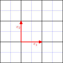
Figure 5. ${\mathcal{T}}(\Phi,{\mathbb{Z}}e_{1}\oplus{\mathbb{Z}}e_{2})$ versus ${\mathcal{T}}(\Phi,{\mathbb{Z}}e_{1}\oplus{\mathbb{Z}}\frac{(e_{1}+e_{2})}{2})$

Definition 5.2.

A function $f$ on $V_{{\mathrm{reg}},{\mathrm{aff}}}$ is called piecewise polynomial with respect to ${\mathcal{H}}_{{\mathrm{aff}}}(\Phi)$ and $\Lambda$ if $f$ coincide with a polynomial function $f^{\tau}$ on each tope $\tau$ in ${\mathcal{T}}(\Phi,\Lambda)$.

A distribution $D$ is called piecewise polynomial with respect to ${\mathcal{H}}(\Phi)$ and $\Lambda$ (in short $({\mathcal{H}},\Lambda)$, or equivalently $(\Phi,\Lambda)$) if it is given by integration on $V_{{\mathrm{reg}},{\mathrm{aff}}}$ by a piecewise polynomial function. The space of piecewise polynomial distributions with respect to $({\mathcal{H}},\Lambda)$ is invariant under translation by $\Lambda$. More generally, if $\Lambda_{1}\subset\Lambda_{2}$, and $D$ is piecewise polynomial with respect to $({\mathcal{H}},\Lambda_{1})$, then ${\rm t}(\lambda_{2})D$ is piecewise polynomial with respect to $(\mathcal{H},\Lambda_{2})$ for any $\lambda_{2}\in\Lambda_{2}$.

The condition for a distribution $b$ to be piecewise polynomial is stronger than the condition that the restriction of $b$ to any tope is a polynomial density. For example the $\delta$ function of the lattice $\Lambda$ restricts to $0$ on any tope $\tau$, but is not a piecewise polynomial distribution.

Let $\phi\in\Phi$, and consider the two arrangements $\mathcal{H}^{\prime}$ and $\mathcal{H}_{0}$ associated to $\phi$ as in the previous section. If $f$ is piecewise polynomial for $(\mathcal{H}^{\prime},\Lambda)$, then $f$ is piecewise polynomial for $(\mathcal{H},\Lambda)$. If $f_{0}$ is piecewise polynomial for $(\mathcal{H}_{0},\Lambda_{0})$, then $p^{*}f$ is piecewise polynomial for $(\mathcal{H},\Lambda)$.

We now prove that $\mathcal{B}(\mathcal{H},\Lambda,g)$ is piecewise polynomial with respect to $(\mathcal{H},\Lambda)$ when $\Phi$ generates $V$ and $g$ is in some subspace of $R_{\mathcal{H}}$ that we describe now.

We may assume that all equations $\phi=0$ of the hyperplanes $H_{\phi}$ in $\mathcal{H}$ lie in $\Lambda$, we can always achieve this by taking an appropriate multiple of $\phi$. Thus, for what follows, we may assume that elements of $\Phi$ are in fact in $\Lambda$.

We denote by $\mathfrak{B}(\Phi)$ the set of subsets of $r$ linearly independent elements of $\Phi$. In other words, an element of $\mathfrak{B}(\Phi)$ is a basis of $V$ extracted from $\Phi$.

Suppose $L$ is a sequence of elements of $\Phi$ (possibly with multiplicities) generating $V$. Define

$$\theta(L)(x)=\frac{1}{\prod_{\alpha\in L}\langle\alpha,x\rangle},$$

a function in $R_{\mathcal{H}}$.

Since $\theta(L)$ will change by a scalar multiple when elements of $L$ are scaled, we may define the following space which depends only on ${\mathcal{H}}$.

Definition 5.3.

Let $G_{\mathcal{H}}$ be the subspace of $R_{\mathcal{H}}$ generated by all rational functions of the form $\theta(L)$.

We recall the following description of $G_{\mathcal{H}}$.

Lemma 5.4.

Any $\theta(L)$ may be written as a linear combination of elements $\theta(\sigma,{\bf n})=\frac{1}{\alpha_{i_{1}}^{n_{1}}\cdots\alpha_{i_{r}}^{n_{r}}}$ where $\sigma:=[\alpha_{i_{1}},\ldots,\alpha_{i_{r}}]\in\mathfrak{B}(\Phi)$ is a basis extracted from $\Phi$ and ${\bf{n}}=[n_{1},n_{2},\ldots,n_{r}]$ is a sequence of positive integers.

Proof.

By induction on the number of elements of $L$, we need to prove that the assertion holds for rational fractions of the form $\theta(\sigma,{\bf n})\frac{1}{\alpha^{N}}$ with $\sigma=[\alpha_{1},\ldots,\alpha_{r}]$ is a basis of $V$. We write $\alpha=\sum_{i=1}^{r}c_{i}\alpha_{i}$. Using the relation,

$$\theta(\sigma,{\bf n})\frac{1}{\alpha^{N}}=\frac{\alpha}{\alpha_{1}^{n_{1}}\cdots\alpha_{r}^{n_{r}}}\frac{1}{\alpha^{N+1}}=\sum_{i,c_{i}\neq 0}c_{i}\frac{1}{\alpha_{1}^{n_{1}}\cdots\alpha_{i}^{n_{i}-1}\cdots\alpha_{r}^{n_{r}}}\frac{1}{\alpha^{N+1}},$$

we decrease the number $|{\bf{n}}|=n_{1}+\cdots+n_{r}$. When one of the $n_{i}$ in the sum becomes $0$, the corresponding term is of the required form associated to the basis $\sigma_{i}=\sigma\cup\{\alpha\}\setminus\{\alpha_{i}\}$. ∎

Proposition 5.5.

If $g\in G_{\mathcal{H}}$, the distribution

$$\mathcal{B}(\mathcal{H},\Lambda,g)(v)=\sum_{\gamma\in\Gamma_{{\mathrm{reg}}}(\mathcal{H})}g(\gamma)e^{2i\pi\langle\gamma,v\rangle}$$

is a piecewise polynomial distribution (with respect to the system $(\mathcal{H},\Lambda)$).

Proof.

We prove the proposition by induction on the number of elements in $\mathcal{H}$. Using Lemma 5.4, it suffices to prove the proposition for $g$ of the form $g=\theta(\sigma,{\bf n})$ for $\sigma\in\mathfrak{B}(\Phi)$ and ${\bf n}$ a sequence of positive integers.

We first assume that $\Phi$ consists of independent elements $\alpha_{1},\alpha_{2},\ldots,\alpha_{r}$ possibly with multiplicities. Consider an element $g=\theta(L)$ of $G_{\mathcal{H}}$ for

$$L=[\alpha_{1},\ldots,\alpha_{1},\alpha_{2},\ldots,\alpha_{2},\ldots,\alpha_{r},\ldots,\alpha_{r}]$$

where $\alpha_{i}$ appears with multiplicity $k_{i}$ in $\Phi$.

Let $\Lambda^{\prime}={\mathbb{Z}}\alpha_{1}\oplus{\mathbb{Z}}\alpha_{2}\oplus\cdots\oplus{\mathbb{Z}}\alpha_{r}$; clearly $\Lambda^{\prime}$ is a sublattice of $\Lambda$. We choose coordinates $t=\sum_{i}t_{i}\alpha_{i}$. Then $\mathcal{B}(\mathcal{H},\Lambda^{\prime},g)=B(t)$ with

(5.5.1) $$B(t)=(-1)^{r}\prod_{i=1}^{r}\frac{1}{k_{i}!}B(k_{i},t_{i}-[t_{i}]).$$

The function $B(t)$ is a polynomial function on each parallelogram translated from the parallelogram $\sum_{i=1}^{r}[0,1]\alpha_{i}$. By equation (7.5.1), the distribution $\mathcal{B}(\mathcal{H},\Lambda,g)$ is obtained by averaging $\mathcal{B}(\mathcal{H},\Lambda^{\prime},g)$ over $\Lambda/\Lambda^{\prime}$. Thus $\mathcal{B}(\mathcal{H},\Lambda,g)$ is piecewise polynomial with respect to $(\mathcal{H},\Lambda)$.

We now consider the general case, where the cardinality of $\mathcal{H}$ is greater than $r$. In this case there exists $\phi\in\Phi$ with the property that, for the hyperplane arrangements ${\mathcal{H}}^{\prime}$ and ${\mathcal{H}}_{0}$ associated to $\phi$, we have $g\in G_{\mathcal{H}^{\prime}}$ and $g_{0}$ (the restriction of $g$ to $\phi=0$) is in $G_{\mathcal{H}_{0}}$. Then, using Proposition 4.3, which states

$$\mathcal{B}(\mathcal{H},\Lambda,g)=\mathcal{B}(\mathcal{H}^{\prime},\Lambda,g)-p^{*}\mathcal{B}(\mathcal{H}_{0},\Lambda_{0},g_{0}),$$

we conclude by induction that $\mathcal{B}(\mathcal{H},\Lambda,g)$ is piecewise polynomial with respect to $({\mathcal{H}},\Lambda)$. ∎

The Bernoulli series $\mathcal{B}(\Phi,\Lambda)$ is equal to $\mathcal{B}(\mathcal{H},\Lambda,g)$ with $g=\frac{1}{\prod_{\phi\in\Phi}\phi}$; it is an element of $G_{\mathcal{H}}$ for we assumed that $\Phi$ spans $V$. Thus, by Proposition 5.5, we immediately obtain that $\mathcal{B}(\Phi,\Lambda)$ is a piecewise polynomial density.

Corollary 5.6.

For any $f\in R_{\mathcal{H}}$, the distribution $\mathcal{B}(\mathcal{H},\Lambda,f)(v)$ restricts to a tope $\tau$ as a polynomial density.

Proof.

Let $f\in R_{\mathcal{H}}$. We can write $f$ as $Pg$ where $P$ is a polynomial and $g\in G_{\mathcal{H}}$. Then the distribution $\mathcal{B}(\mathcal{H},\Lambda,f)(v)$ is obtained by applying the differential operator $P(\partial_{v})$ to the distribution $\mathcal{B}(\mathcal{H},\Lambda,g)(v)$.

This differentiation is in the distribution sense so that it may produce distributions supported on admissible hyperplanes, but on an open tope $\tau$, we obtain a polynomial density. ∎

Definition 5.7.

Given a tope $\tau$ in ${\mathcal{T}}(\Phi,\Lambda)$, we denote by $\operatorname{Ber}(\Phi,\Lambda,\tau)$ the polynomial function on $V$ such that the restriction of $\mathcal{B}(\Phi,\Lambda)$ to $\tau$ coincides with the restriction of $\operatorname{Ber}(\Phi,\Lambda,\tau)(v)d_{\Lambda}v$ on $\tau$.

By the above proof, we see that the polynomial $\operatorname{Ber}(\Phi,\Lambda,\tau)$ is of degree equal to the number of elements in $\Phi$.

The fact that $\mathcal{B}(\Phi,\Lambda)(v)$ is a periodic distribution on $V$ implies immediately the following periodicity formula. For any $\lambda\in\Lambda$ and $v\in V$,

(5.7.1) $$\operatorname{Ber}(\Phi,\Lambda,\tau+\lambda)(v+\lambda)=\operatorname{Ber}(\Phi,\Lambda,\tau)(v).$$

If $\nu$ is a connected subset of $V$ contained in the open set of regular elements, we denote by $\operatorname{Ber}(\Phi,\Lambda,\nu)$ the polynomial $\operatorname{Ber}(\Phi,\Lambda,\tau(\nu))$ where $\tau(\nu)$ is the unique tope containing $\nu$.

Let $\tau\in{\mathcal{T}}(\Phi,\Lambda)$ and $\phi\in\Phi$. If $v_{0}\in V_{0}=V/<\phi>$ is the projection of $v\in\tau$, then $v_{0}$ is not on any affine wall in $V_{0}$. Indeed the reciproc image of an affine wall in $V_{0}$ is an affine wall in $V$. We denote by $\tau_{0}$ the unique tope in $V_{0}$ containing the projection of $\tau$.

Equation (3.1.1) implies the following relations.

If $\Phi-\{\phi\}$ generates $V$, then

(5.7.2) $$\partial_{\phi}\operatorname{Ber}(\Phi,\Lambda,\tau)=\operatorname{Ber}(\Phi-\{\phi\},\Lambda,\tau)-\operatorname{Ber}(\Phi_{0},\Lambda_{0},\tau_{0}).$$

If $\Phi$ generates $V$, but $\Phi-\{\phi\}$ does not generate $V$, then

(5.7.3) $$\partial_{\phi}\operatorname{Ber}(\Phi,\Lambda,\tau)=-\operatorname{Ber}(\Phi_{0},\Lambda_{0},\tau_{0}).$$

Remark 5.8.

By using reduction to independent variables and the explicit formula (5.5.1), we obtain also a way to compute $\operatorname{Ber}(\Phi,\Lambda,\tau)$. This can be applied not too painfully when the number of elements in $\Phi$ is small. However, the residue formula due to A. Szenes [12] to compute $\operatorname{Ber}(\Phi,\Lambda,\tau)$ is very efficient when $\Phi$ is large, provided the dimension of $V$ is relatively small. We will give examples of computations of volumes of moduli spaces using Szenes formula in a next article.

6. An Euler-MacLaurin formula

This section is independent of the rest of the article.

Assume that $\Phi$ generates $V$. Using the Lebesgue measure associated to the lattice $\Lambda$, we identify $\mathcal{B}(\Phi,\Lambda)(v)$ to a piecewise polynomial function on $V$.

Let us denote by ${\mathcal{R}}$ the set of $\Phi$-admissible subspaces of $V$. Then $\mathfrak{s}=V$ and $\mathfrak{s}=\{0\}$ are the maximum and minimum elements of the partially ordered set ${\mathcal{R}}$. If $\mathfrak{s}$ is a $\Phi$-admissible subspace of $V$, we denote by $\Phi\setminus\mathfrak{s}$ the sequence of elements in $\Phi$ not lying in the space $\mathfrak{s}$.

The projection of the list $\Phi\setminus\mathfrak{s}$ on $V/\mathfrak{s}$ will be denoted by $\Phi/\mathfrak{s}$. The image of the lattice $\Lambda$ in $V/\mathfrak{s}$ is a lattice in $V/\mathfrak{s}$. If $\Phi$ generates $V$, $\Phi/\mathfrak{s}$ generates $V/\mathfrak{s}$. Using the projection $V\to V/\mathfrak{s}$, we identify the piecewise polynomial function ${\mathcal{B}}(\Phi/\mathfrak{s},\Lambda/\mathfrak{s})$ on $V/\mathfrak{s}$ to a piecewise polynomial function on $V$ constant along the affine spaces $v+\mathfrak{s}$. Then,

$$\Gamma_{\rm reg}(\Phi/\mathfrak{s}):=\Gamma\cap U_{\rm reg}(\Phi/\mathfrak{s})$$

is the set of elements $\gamma\in\Gamma$ satisfying ${\langle}\gamma,s{\rangle}=0$ for all $s\in\mathfrak{s}$ and ${\langle}\gamma,\phi{\rangle}\neq 0$ for all $\phi\in\Phi\setminus\mathfrak{s}$.

We lift functions on $V/\mathfrak{s}$ to functions on $V$ by the canonical projection. Thus ${\mathcal{B}}(\Phi/\mathfrak{s},\Lambda/\mathfrak{s})$ is the function on $V$ given by the series (convergent in the sense of generalized functions)

$$\sum_{\gamma\in\Gamma_{\rm reg}(\Phi/\mathfrak{s})}\frac{e^{2i\pi{\langle}v,\gamma{\rangle}}}{\prod_{\phi\in\Phi\setminus\mathfrak{s}}2i\pi{\langle}\phi,\gamma{\rangle}}.$$

This function is periodic with respect to the lattice $\Lambda$, piecewise polynomial on $V$ (relative to ($\Phi$,$\Lambda$)) and constant along $v+\mathfrak{s}$. We denote it simply by $\mathcal{B}(\Phi/\mathfrak{s})$ leaving its dependence on the lattice $\Lambda$ implicit. If $\mathfrak{s}=V$, the function ${\mathcal{B}}(\Phi/\mathfrak{s})$ is identically equal to $1$; if $\mathfrak{s}=\{0\}$, then we obtain the multiple Bernoulli series $\mathcal{B}(\Phi,\Lambda)$.

Theorem 6.1.

Let $f$ be a smooth function on $V$, rapidly decreasing with rapidly decreasing derivatives. Then,

$$\sum_{\lambda\in\Lambda}f(\lambda)=\sum_{\mathfrak{s}\in{\mathcal{R}}}(-1)^{|\Phi\setminus\mathfrak{s}|}\int_{V}{\mathcal{B}}(\Phi/\mathfrak{s})(v)(\prod_{\phi\in\Phi\setminus\mathfrak{s}}\partial_{\phi})f(v)dv.$$

Remark 6.2.

The term corresponding to $\mathfrak{s}=V$ in the above sum gives the term $\int_{V}f(v)dv$. Thus we may also write the formula as

$$\sum_{\lambda\in\Lambda}f(\lambda)-\int_{V}f(v)dv=\sum_{\mathfrak{s}\neq V}(-1)^{|\Phi\setminus\mathfrak{s}|}\int_{V}{\mathcal{B}}(\Phi/\mathfrak{s})(v)(\prod_{\phi\in\Phi\setminus\mathfrak{s}}\partial_{\phi})f(v)dv.$$

All the sets $\Phi\setminus\mathfrak{s}$ entering in this formula are ‘long’, that is, their complement in $\Phi$ do not generate $V$. In particular they contain a ‘cocircuit’. This formula has been used in [16] to obtain a formula for the semi-discrete convolution with the Box Spline.

Proof.

Let

$$\hat{f}(y)=\int_{V}e^{2i\pi\langle y,x\rangle}f(x)dx.$$

By Poisson formula

$$\sum_{\lambda\in\Lambda}f(\lambda)=\sum_{\gamma\in\Gamma}\hat{f}(\gamma).$$

We group together the terms in $\Gamma$ belonging to $\mathfrak{s}^{\perp}$ for $\mathfrak{s}\in{\mathcal{R}}$. More precisely, the lattice $\Gamma$ is a disjoint union over the $\mathfrak{s}\in{\mathcal{R}}$ of the sets

$$\Gamma_{{\mathrm{reg}}}(\Phi/\mathfrak{s})=\{\gamma\in\mathfrak{s}^{\perp}\cap\Gamma|{\langle}\phi,\gamma{\rangle}\neq 0\;\text{for all}\;\phi\in\Phi\setminus\mathfrak{s}\}.$$

Now in the generalized sense

$$\sum_{\gamma\in\Gamma_{{\mathrm{reg}}}(\Phi/\mathfrak{s})}\hat{f}(\gamma)=\int_{V}\sum_{\gamma\in\Gamma_{{\mathrm{reg}}}(\Phi/\mathfrak{s})}e^{2i\pi{\langle}v,\gamma{\rangle}}f(v)dv$$

$$=\int_{V}\partial_{\Phi\setminus\mathfrak{s}}{\mathcal{B}}(\Phi/\mathfrak{s})(v)f(v)$$

and we obtain the statement in the theorem. ∎

7. Wall crossing

In this section we again assume that $\Phi$ generates $V$. Under this assumption, we compare the polynomials $\operatorname{Ber}(\Phi,\Lambda,\tau)$ associated to two adjacent topes of ${\mathcal{T}}(\Phi,\Lambda)$ separated by an hyperplane $W$. We remark that due to the periodicity property of $\mathcal{B}(\Phi,\Lambda)$ it suffices to consider jumps over an hyperplane $W$ passing through the origin.

If $D_{1}$ and $D_{2}$ are two distributions on $V$ with supports $S_{1}$ and $S_{2}$ with the property that for any $v\in V$ the intersection of $v-S_{1}$ and $S_{2}$ lies in a compact set, then the convolution $D_{1}*D_{2}$ is well defined.

We recall the definition of multispline. Let $X=[v_{1},v_{2},\ldots,v_{m}]$ be a sequence of non-zero vectors in $V$. We will first consider the case where $X$ spans a pointed cone. The multivariate spline $T(X)$ is the tempered distribution defined on test functions $f$ by:

(7.0.1) $$\langle T(X)\,|\,f\rangle=\int_{0}^{\infty}\cdots\int_{0}^{\infty}f(\sum_{i=1}^{m}t_{i}v_{i})dt_{1}\cdots dt_{m}.$$

If $X$ spans $V$, we may interpret $T(X)$ as a function on $V$ supported in the cone $C(X)$ generated by $X$. This function is piecewise polynomial. If $v\in X$, then $\partial_{v}T(X)=T(X-\{v\})$. When $X$ is the empty set, $T(X)=\delta_{0}$.

We now consider the case where the elements of $X$ do not necessarily lie in a half-space. We introduce a polarization of $X$ given by a vector $u$ in $U$. Let $u\in U$ be a vector that is nonzero on all elements of $X$. We will then say that the vector $u$ is polarizing for $X$. Divide the list $X$ into two lists $A$ and $B$, the lists of positive and negative vectors on $u$ respectively. We then define

$$T(X,u)=(-1)^{|B|}T([A,-B]).$$

Example 7.1.

With the notation of Example 2.2,

$$T(\Phi_{k},\omega^{*})=\begin{cases}&\frac{t^{k-1}}{(k-1)!}\;\;\text{if $t>0$,}\\ &0\;\;\;\;\text{if $t<0$}\end{cases}\;\;\text{and}\;\;T(\Phi_{k},-\omega^{*})=\begin{cases}&0\;\;\;\;\text{if $t>0$,}\\ &-\frac{t^{k-1}}{(k-1)!}\;\;\text{if $t<0$.}\\ \end{cases}$$

We return to our set up. Let $\Phi$ be a sequence of nonzero vectors in $V$, spanning $V$. Let $W$ be a $\Phi$-admissible hyperplane. Let $E\in\Gamma$ be an equation of this hyperplane, where $E$ is a primitive vector in $\Gamma$; this fixes $E$ up to sign. The lattice $\Lambda$ is fixed, and we write simply $dv$ instead of $d_{\Lambda}v$. Similarly we denote by $dh$ the density determined by $\Lambda\cap W$. As $E$ does not vanish on any element of $\Phi\setminus W$, we may define $T(\Phi\setminus W,E)$ as above; it is a distribution supported on $E\geq 0$. Let $p$ be a polynomial density on $W$. Then, the convolution $p*T(\Phi\setminus W,E)$ is well defined and it is supported on $E\geq 0$. Similarly, $p*T(\Phi\setminus W,-E)$ is supported on $E\leq 0$. It is easily proven (see [1]) that $p*T(\Phi\setminus W,E)-p*T(\Phi\setminus W,-E)$ is given by integration against a polynomial density. We thus define the polynomial ${\rm Pol}(p,\Phi\setminus W,E)$ by the equation

$${\rm Pol}(p,\Phi\setminus W,E)(v)dv=p*T(\Phi\setminus W,E)-p*T(\Phi\setminus W,-E).$$

The following properties of ${\rm Pol}(p,\Phi\setminus W,E)$ follow directly from the above equation.

Lemma 7.2.

Let $\Psi=\Phi\setminus W$.

(a)Let $\psi\in\Psi$. Then,

$$\partial_{\psi}{\rm Pol}(p,\Psi,E)={\rm Pol}(p,\Psi-\{\psi\},E).$$

(b) If $\Psi=[\psi]$, then for $h\in W$ and $t\in{\mathbb{R}}$,

$${\rm Pol}(p,\{\psi\},E)(h+t\psi)=\frac{f(h)}{{\langle}\psi,E{\rangle}}$$

if $p(h)=f(h)dh.$

(c) If $|\Psi|>1$, then the restriction of ${\rm Pol}(p,\Psi,E)$ to $W$ vanishes of order $|\Psi|-1$.

The following one dimensional residue formula for ${\rm Pol}(p,\Phi\setminus W,E)$ is given in [1]. It is useful in computing the convolutions. We write $p(h)=f(h)dh$ where $f$ is a polynomial function on the hyperplane $W$.

Lemma 7.3.

Let $P$ be a polynomial function on $V$ extending $f$. Then, for $v\in V$,

$${\rm Pol}(p,\Phi\setminus W,E)(v)=\operatorname{Res}_{z=0}\left(\left(P(\partial_{x})\cdot\frac{e^{\langle v,x+zE\rangle}}{\prod_{\phi\in\Phi\setminus W}\langle\phi,x+zE\rangle}\right)_{x=0}\right).$$

Theorem 7.4.

Let $\tau_{1}$ and $\tau_{2}$ be two adjacent topes in ${\mathcal{T}}(\Phi,\Lambda)$ separated by the hyperplane $W$ defined by $E$ with ${\langle}v,E{\rangle}>0$ for any $v\in\tau_{1}$. Denote by $\tau_{12}$ the tope in ${\mathcal{T}}(\Phi\cap W,\Lambda\cap W)$ containing $\overline{\tau_{1}}\cap\overline{\tau_{2}}$ in its closure. Let $\operatorname{Ber}^{\tau_{12}}:=\operatorname{Ber}(\Phi\cap W,\Lambda\cap W,\tau_{12})dh$ be the polynomial density on $W$ determined by $\tau_{12}$. Then,

(7.4.1) $$(\operatorname{Ber}(\Phi,\Lambda,\tau_{1})-\operatorname{Ber}(\Phi,\Lambda,\tau_{2}))dv=\operatorname{Ber}^{\tau_{12}}*T(\Phi\setminus W,E)-\operatorname{Ber}^{\tau_{12}}*T(\Phi\setminus W,-E).$$

Remark 7.5.

Formula (7.4.1) is very similar to jump formulae for volume of reduced spaces in Hamiltonian geometry. Indeed if $\mu:M\to\mathfrak{t}^{*}$ is a proper moment map associated to an Hamiltonian action of a torus $T$, then the set of regular values of $\mu$ is the complement of a certain number of affine hyperplanes. On each connected component, volumes of reduced spaces $M_{red}(v):=\mu^{-1}(v)/T$ are given by polynomial functions of $v$. When crossing a wall, the variation of these polynomials follow the same jump scheme as in equation (7.4.1): they are determined by a polynomial volume function associated to a smaller Hamiltonian manifold $M_{0}$ and weights of the normal bundle of $M_{0}$ in $M$ ([9]). In particular, when the sequence $\Phi$ is comprised of positive coroots of a compact connected Lie group $G$ with multiplicity $2g-1$ and $\Lambda$ is the coroot lattice of $G$, the polynomials $\operatorname{Ber}(\Phi,\Lambda,\tau)$ describe (up to some normalization) the symplectic volume of the moduli space of flat $G$-connections on Riemann surface of genus $g$ with one boundary component, around which the holonomy is determined by $v$. These moduli spaces are reduced spaces $M_{red}(v)$ of an Hamiltonian action.

Proof.

We will first verify the claim for the case where there is only one vector $\phi$ in $\Phi$ that is not contained in $W$.

Let $\Lambda_{0}=\Lambda\cap W$. We consider the lattice $\Lambda_{b}=\Lambda_{0}\oplus{\mathbb{Z}}\phi.$ By formula (2.1.1),

(7.5.1) $$\mathcal{B}(\Phi,\Lambda)(v)=\sum_{\lambda_{j}\in\Lambda/\Lambda_{b}}\mathcal{B}(\Phi,\Lambda_{b})(v+\lambda_{j}).$$

For $t$ in a small neighborhood of zero, let $\tau_{1}$ (respectively $\tau_{2}$) denote the tope containing the open set of $v=h+t\phi$ for $h\in W$ lying in a relatively compact open subset of $\tau_{12}$ and $t>0$ (respectively $t<0$).

We may express a representative of a non-zero $\lambda_{j}\in\Lambda/\Lambda_{b}$ as $\lambda_{j}=h_{j}+t_{j}\phi$ for $h_{j}\in\Lambda_{0}$ and $t_{j}\notin{\mathbb{Z}}$. As the lattice $\Lambda_{b}$ is product of lattices, we have

$$\mathcal{B}(\Phi,\Lambda_{b})(h+t\phi)=\mathcal{B}(\Phi\cap W,\Lambda_{0})(h)(-t+[t]+\frac{1}{2})dt.$$

Observe that the jump in the function $\mathcal{B}(\Phi,\Lambda_{b})(v+\lambda_{j})=\mathcal{B}(\Phi,\Lambda_{b})(h+h_{j}+(t+t_{j})\phi)$ as $t$ changes sign in a small neighborhood of zero is precisely zero for the nontrivial representative $\lambda_{j}$ since $t_{j}$ is not integral. Thus the only contribution to the jump comes from the trivial $\lambda_{j}$ in the sum of equation (7.5.1). We get

$$\operatorname{Ber}(\Phi,\Lambda,\tau_{1})(v)-\operatorname{Ber}(\Phi,\Lambda,\tau_{2})(v)=\\ \frac{1}{\langle E,\phi\rangle}\operatorname{Ber}(\Phi\cap W,\Lambda_{0})(h)((-t+\frac{1}{2}-(-t-\frac{1}{2})).$$

The convolution product in this case is just the product in coordinates so that

$$\operatorname{Ber}(\Phi\cap W,\Lambda_{0},\tau_{12})*T(\{\phi\},E)-\operatorname{Ber}(\Phi\cap W,\Lambda_{0},\tau_{12})(h)*T(\{\phi\},-E)$$

is equal at the point $(h,t)$ to $\operatorname{Ber}(\Phi\cap W,\Lambda_{0},\tau_{12})(h)$ and hence we obtain the claimed formula.

Now consider the case where there are several elements of $\Phi$ that do not lie in $W$. Let $\phi$ be a vector in $\Phi\setminus W$. Let $\Phi^{\prime}=\Phi-\{\phi\}$; $\Phi^{\prime}$ still generates $V$ and $\Phi^{\prime}\cap W=\Phi\cap W$. Equation (3.1.1) implies that in this case $\mathcal{B}(\Phi,\Lambda)$ is continuous on $W$: indeed the derivative in the direction $\phi$ is a piecewise polynomial function.

Let $\tau_{1}^{\prime}$ and $\tau_{2}^{\prime}$ be the topes of $\Phi^{\prime}$ containing $\tau_{1}$ and $\tau_{2}$ respectively. They are adjacent with respect to $W$ and $\operatorname{Ber}^{\tau_{12}}=\operatorname{Ber}^{\tau_{12}^{\prime}}$. Using equation (5.7.2), we have

$$\partial_{\phi}\operatorname{Ber}(\Phi,\Lambda,\tau_{1})-\partial_{\phi}\operatorname{Ber}(\Phi,\Lambda,\tau_{2})=\operatorname{Ber}(\Phi^{\prime},\Lambda,\tau_{1}^{\prime})-\operatorname{Ber}(\Phi^{\prime},\Lambda,\tau_{2}^{\prime}).$$

Indeed the topes $\tau_{1}$ and $\tau_{2}$ give the same tope $\tau_{0}$ under projection onto $V_{0}=V/<\phi>$.

By Lemma 7.2 part $(a)$,

$$\partial_{\phi}{\rm Pol}(\operatorname{Ber}^{\tau_{12}},\Phi\setminus W,E)={\rm Pol}(\operatorname{Ber}^{\tau^{\prime}_{12}},\Phi^{\prime}\setminus W,E).$$

Denote by ${\rm Leq}(\Phi)$ the left hand side, and by ${\rm Req}(\Phi)$ the right hand side of equation (7.4.1). By induction, we have $\partial_{\phi}({\rm Leq}(\Phi)-{\rm Req}(\Phi))=0$. Thus, the polynomial function is constant in the direction of ${\mathbb{R}}\phi$. The left hand side vanishes on $W$ by the continuity of $\mathcal{B}(\Phi,\Lambda)$ on $W$. Hence the claim. ∎

We now demonstrate the theorem with various examples.

Example 7.6.

Recall the data of Example 2.2. Let $\tau_{1}$ and $\tau_{2}$ be two adjacent topes defined by inequalities $0<t<1$ and $-1<t<0$ respectively. By Theorem 7.4 and Example 7.1,

$$\operatorname{Ber}(\Phi,\Lambda,\tau_{1})(t\omega)-\operatorname{Ber}(\Phi,\Lambda,\tau_{2})(t\omega)=\frac{t^{k-1}}{(k-1)!},$$

which is indeed equal to $-\frac{1}{k!}B(k,t)+\frac{1}{k!}B(k,t+1)$ as it can be seen from the explicit expression of $\mathcal{B}(\Phi_{k},\Lambda)(t\omega)$ in Example 2.2.

Example 7.7.

Recall the data of Example 2.3. Let $\tau_{1}$ and $\tau_{2}$ be the two adjacent topes separated by the hyperplane $W={\mathbb{R}}(e_{1}+e_{2})$ (see figure 6(a)). Then $E=-e^{1}+e^{2}$.

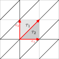
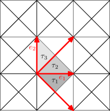
(a)                                               (b)

Figure 6. ${\mathcal{T}}([e_{1},e_{2},e_{1}+e_{2}],\Lambda)$ versus ${\mathcal{T}}([e_{1},e_{2},e_{1}+e_{2},e_{1}-e_{2}],\Lambda)$ with $\Lambda={\mathbb{Z}}e_{1}\oplus{\mathbb{Z}}e_{2}$

We express $v=v_{1}e_{1}+v_{2}e_{2}\in V$ as $v=v_{1}(e_{1}+e_{2})+(v_{2}-v_{1})e_{2}$ and $x\in U$ as $x=x_{1}e^{1}+x_{2}(-e^{1}+e^{2})$. Using Example 2.2, with $\Phi\cap W=e_{1}+e_{2}$ and $\Lambda\cap W={\mathbb{Z}}(e_{1}+e_{2})$ at $v_{1}(e_{1}+e_{2})$, we have

$$\begin{array}[]{ll}\operatorname{Ber}^{\tau_{12}}&=\operatorname{Ber}(\Phi\cap W,\Lambda\cap W,\tau_{12})(v_{1}(e_{1}+e_{2}))\\ &=\frac{1}{2}-v_{1}\end{array}$$

In the above coordinates of $U$, the operator $\operatorname{Ber}^{\tau_{12}}(\partial_{x})=\frac{1}{2}-\partial_{x_{1}}$ under the identification $P(\partial_{x})e^{{\langle}a,x{\rangle}}=P(a)e^{{\langle}a,x{\rangle}}$. Then,

$$\begin{array}[]{ll}{\rm Pol}(\operatorname{Ber}^{\tau_{12}},\Phi,E)(v)&=\operatorname{Res}_{z=0}\left(\left(\operatorname{Ber}^{\tau_{12}}(\partial_{x})\cdot\frac{e^{{\langle}v,x+zE{\rangle}}}{\prod_{\phi\in\Phi\setminus W}{\langle}\phi,x+zE{\rangle}}\right)_{x=0}\right)\\ &=\operatorname{Res}_{z=0}\left(\left((\frac{1}{2}-\partial{x_{1}})\cdot\frac{e^{v_{1}x_{1}+(v_{2}-v_{1})x_{2}+(v_{2}-v_{1})z}}{(x_{1}-x_{2}-z)(x_{2}+z)}\right)_{x=0}\right)\\ &=\operatorname{Res}_{z=0}\left(\left((\frac{1}{2}-\partial{x_{1}})\cdot\frac{e^{v_{1}x_{1}+(v_{2}-v_{1})z}}{(x_{1}-z)z}\right)_{x_{1}=0}\right)\\ &=\frac{1}{2}(1-v_{1}-v_{2})(v_{1}-v_{2}),\end{array}$$

which is indeed the jump $\operatorname{Ber}(\Phi,\Lambda,\tau_{1})(v)-\operatorname{Ber}(\Phi,\Lambda,\tau_{2})(v)$ as it can be seen from the explicit expression in Example 2.3.

Example 7.8.

Recall the data of Example 2.4.

(a) Jump over the wall $W={\mathbb{R}}e_{1}$: Then $E=e^{2}$, $\Phi\cap W=\{e_{1}\}$ and $\Lambda\cap W={\mathbb{Z}}e_{1}$ (see figure 6(b)).

$$\begin{array}[]{ll}{\rm Pol}(Ber^{\tau_{21}},\Phi,E)(a)&=\operatorname{Res}_{z=0}\left(Ber^{\tau_{21}}(\partial_{x})\cdot\frac{e^{{\langle}a,x+ze^{2}{\rangle}}}{\prod_{\phi\in\Phi\setminus\Phi\cap W}{\langle}\phi,x+zE{\rangle}}\right)_{x=0}\\ &=\operatorname{res}_{z=0}\left((-\partial_{x_{1}}+\frac{1}{2})\cdot\frac{e^{v_{1}x_{1}+v_{2}x_{2}+v_{2}z}}{(x_{2}+z)(x_{1}+x_{2}+z)(x_{1}-x_{2}-z)}\right)_{x_{2}=0}\\ &=\frac{1}{4}v_{2}^{2}(2v_{1}-1),\end{array}$$

which is indeed the jump $\operatorname{Ber}(\Phi,\Lambda,\tau_{2})(v)-\operatorname{Ber}(\Phi,\Lambda,\tau_{1})(v)$ as it can be seen from the explicit expression in Example 2.4.

(b) Jump over the wall $W={\mathbb{R}}(e_{1}+e_{2})$: Then $E=-e^{1}+e^{2}$. We express $v=v_{1}e_{1}+v_{2}e_{2}\in V$ as $v=v_{1}(e_{1}+e_{2})+(v_{2}-v_{1})e_{2}$ and $x\in U$ as $x=x_{1}e^{1}+x_{2}(-e^{1}+e^{2})$. Using Example 2.2, with $\Phi\cap W=e_{1}+e_{2}$ and $\Lambda\cap W={\mathbb{Z}}(e_{1}+e_{2})$ at $v_{1}(e_{1}+e_{2})$, we have $\operatorname{Ber}^{\tau_{23}}=\operatorname{Ber}(\Phi\cap W,\Lambda\cap W,\tau_{23})(v_{1}(e_{1}+e_{2}))=\frac{1}{2}-v_{1}$. Then,

$$\begin{array}[]{ll}{\rm Pol}(\operatorname{Ber}^{\tau_{23}},\Phi,E)(v)&=\operatorname{Res}_{z=0}\left(\left((\frac{1}{2}-\partial{x_{1}})\cdot\frac{e^{v_{1}x_{1}+(v_{2}-v_{1})x_{2}+(v_{2}-v_{1})z}}{(x_{1}-x_{2}-z)(x_{2}+z)(x_{1}-2x_{2}-2z)}\right)_{x=0}\right)\\ &=-\frac{1}{8}(v_{1}-1+v_{2})(v_{1}-v_{2})^{2},\end{array}$$

which is indeed the jump $\operatorname{Ber}(\Phi,\Lambda,\tau_{3})(v)-\operatorname{Ber}(\Phi,\Lambda,\tau_{2})(v)$ as it can be seen from the explicit expression in Example 2.4.

8. The affine case

This section generalizes previous results to the affine case. Results proven here are not needed for the following section.

Let $\Phi=[\phi_{1},\ldots,\phi_{N}]$ be a list of elements of $V_{\mathbb{Q}}$ and let ${\bf z}=[z_{1},z_{2},\ldots,z_{N}]$ be a list of complex numbers. We consider the augmented list $\tilde{\Phi}:=[[\phi_{1},z_{1}],\ldots,[\phi_{N},z_{N}]]$ and define

$$\Gamma_{{\mathrm{reg}}}(\tilde{\Phi})=\Gamma\cap U_{{\mathrm{reg}}}(\tilde{\Phi})$$

where

$$U_{{\mathrm{reg}}}(\tilde{\Phi})=\{u\in U|\;\langle\phi_{j},u\rangle+z_{j}\neq 0\;\mbox{for all}\;j\}.$$

Definition 8.1.

The affine multiple Bernoulli series is the distribution

$$\mathcal{B}(\tilde{\Phi},\Lambda)=\sum_{\gamma\in\Gamma_{{\mathrm{reg}}}(\tilde{\Phi})}\frac{e^{2i\pi\langle v,\gamma\rangle}}{\prod_{j=1}^{N}2i\pi(\langle\phi_{j},\gamma\rangle+z_{j})}d_{\Lambda}v.$$

The distribution $\mathcal{B}(\tilde{\Phi},\Lambda)$ has the following properties, similar to its nonaffine counterpart:

$\bullet$ If $\Phi$ is the empty set, then $\mathcal{B}(\tilde{\Phi},\Lambda)$ is the $\delta$-distribution of the lattice $\Lambda$.

$\bullet$ If $\Lambda_{1}\subset\Lambda_{2}$. Then $\mathcal{B}(\tilde{\Phi},\Lambda_{2})$ is obtained from $\mathcal{B}(\tilde{\Phi},\Lambda_{1})$ by averaging over $\Lambda_{2}/\Lambda_{1}$:

(8.1.1) $$\mathcal{B}(\tilde{\Phi},\Lambda_{2})=\sum_{\lambda_{2}\in\Lambda_{2}/\Lambda_{1}}{\rm t}(\lambda_{2})\mathcal{B}(\tilde{\Phi},\Lambda_{1}).$$

In the special case $z_{j}=\langle\phi_{j},z\rangle$ for $z\in U_{\mathbb{C}}$, it is more natural to consider the distribution

$$\operatorname{Eis}(\Phi,\Lambda,z)(v)=\sum_{\gamma\in\Gamma;\langle\phi_{j},\gamma+z\rangle\neq 0}\frac{e^{2i\pi\langle v,\gamma+z\rangle}}{\prod_{j=1}^{N}2i\pi\langle\phi_{j},\gamma+z\rangle}.$$

Clearly,

$$\operatorname{Eis}(\Phi,\Lambda,z)(v)=e^{2i\pi\langle v,z\rangle}{\mathcal{B}}(\tilde{\Phi},\Lambda)(v)$$

for $\tilde{\Phi}=[[\phi_{1},\langle\phi_{1},z\rangle],\cdots[\phi_{N},\langle\phi_{N},z\rangle]]$. If $z$ is regular, that is $\langle\phi,\gamma\rangle+z\neq 0$ for all $\phi\in\Phi$, then $\operatorname{Eis}(\Phi,\Lambda,z)(v)$ defines a distribution of $v$ with coefficients meromorphic functions on $T_{\mathbb{C}}=U_{\mathbb{C}}/\Gamma$ which is studied in [3].

Example 8.2.

Let $\Lambda={\mathbb{Z}}\omega$, and let $\tilde{\Phi}_{k}=[[\omega,z],[\omega,z],\ldots,[\omega,z]]$ where $[\omega,z]$ is repeated $k$ times. If $z$ is integral, we simply have

$$\mathcal{B}(\tilde{\Phi}_{k},\Lambda)(t\omega)=e^{-2i\pi zt}\mathcal{B}(\Phi_{k},\Lambda)(t\omega).$$

If $z$ is not integral and $k=1$, then, using Lemma 16 of [3],

(8.2.1) $$\mathcal{B}(\tilde{\Phi}_{1},\Lambda)(t\omega)=\sum_{n\in{\mathbb{Z}}}\frac{e^{2i\pi nt}}{2i\pi(n+z)}dt=\frac{e^{([t]-t)2i\pi z}}{1-e^{-2i\pi z}},$$

which is an analytic function of $t$ in each tope.

If $k>1$, $z$ not integral, and $0<t<1$, we use the residue theorem for the integral

$$\int_{|u|=R}\frac{e^{-tu}}{(2i\pi z-u)^{k}(1-e^{-u})}du$$

which tends to $0$ when $R$ tends to infinity. Then,

$$\begin{array}[]{ll}\mathcal{B}(\tilde{\Phi}_{k},\Lambda)(t\omega)&=-\operatorname{Res}_{u=2i\pi z}\frac{e^{-tu}}{(2i\pi z-u)^{k}(1-e^{-u})}du\\ &=e^{-2i\pi zt}\operatorname{Res}_{u=0}\frac{e^{tu}}{u^{k}(1-e^{-2i\pi z+u})}du.\end{array}$$

Thus, we see that $\mathcal{B}(\tilde{\Phi}_{k},\Lambda)(t\omega)$ is a product of an exponential function of $t$ and a polynomial in $t$. In particular, in the interval $0<t<1$, it is an analytic function of $t$. For example, for $k=2$ and $0<t<1$, we get

$$\mathcal{B}(\tilde{\Phi}_{2},\Lambda)(t\omega)=\frac{e^{-2i\pi zt}}{1-e^{-2i\pi z}}\left(t+\frac{1}{e^{2i\pi z}-1}\right).$$

8.1. Recurrence relations

In the affine case the recurrence relation (3.1.1) is slightly modified.

Let $\tilde{\phi}=[\phi,z]$ be an element of $\tilde{\Phi}$. We consider two cases.

$\bullet$ Suppose there exists $\gamma_{z}\in\Gamma$ such that

(8.2.2) $$\langle\phi,\gamma_{z}\rangle+z=0.$$

Then, we may express $\gamma\in\Gamma_{{\mathrm{reg}}}(\tilde{\Phi}-\{\tilde{\phi}\})$ satisfying ${\langle}\gamma,\phi{\rangle}+z=0$ as $\gamma=\gamma^{\prime}+\gamma_{z}$. Clearly, $\langle\gamma^{\prime},\phi\rangle=0$.

We consider the system

$$\tilde{\Phi}_{0}=[[\overline{\phi}_{j},z_{j}+\langle\phi_{j},\gamma_{z}\rangle],\;\phi_{j}\in\Phi-\{\phi\}]$$

in $V_{0}=V/<\phi>$. The sum

$$\sum_{\gamma^{\prime}\in\Gamma_{{\mathrm{reg}}}(\tilde{\Phi}-\{\tilde{\phi}\}),{\langle}\gamma^{\prime},\phi{\rangle}=0}\frac{e^{{\langle}2i\pi v,\gamma^{\prime}{\rangle}}}{\prod_{\phi_{j}\in\Phi-\{\phi\}}2i\pi({\langle}\phi_{j},\gamma^{\prime}{\rangle}+{\langle}\phi_{j},\gamma_{z}{\rangle}+z_{j})}$$

is constant in the direction of $\phi$ and identifies with $\mathcal{B}(\tilde{\Phi}_{0},\Lambda)(\overline{v})$. Hence, we get the following recurrence relation.

(8.2.3) $$(\partial_{\phi}+2i\pi z)\mathcal{B}(\tilde{\Phi},\Lambda)(v)=\mathcal{B}(\tilde{\Phi}-\{\tilde{\phi}\},\Lambda)(v)-e^{2i\pi\langle v,\gamma_{z}\rangle}\mathcal{B}(\tilde{\Phi}_{0},\Lambda_{0})(\overline{v}).$$

$\bullet$ If there does not exist $\gamma_{z}$ satisfying the relation (8.2.2), then $\Gamma_{{\mathrm{reg}}}(\tilde{\Phi}-\{\tilde{\phi}\})=\Gamma_{{\mathrm{reg}}}(\tilde{\Phi})$, and the equation (8.2.3) reduces to

$$(\partial_{\phi}+2i\pi z)\mathcal{B}(\tilde{\Phi},\Lambda)(v)=\mathcal{B}(\tilde{\Phi}-\{\tilde{\phi}\},\Lambda)(v).$$

8.2. Piecewise exponential polynomial behavior

We consider $\tilde{\phi}=[\phi,z]\in\tilde{\Phi}$ with $\phi\neq 0$. Consider the complex hyperplane $H_{\tilde{\phi}}:=\{u\in U_{\mathbb{C}}:{\langle}u,\phi{\rangle}+z=0\}$. Consider the set

$$\tilde{\mathcal{H}}={\mathcal{H}}(\tilde{\Phi})=\{H_{\tilde{\phi}},\;\tilde{\phi}\in\tilde{\Phi}\}$$

of hyperplanes in $U_{\mathbb{C}}$. We denote by $\mathcal{R}_{\tilde{{\mathcal{H}}}}$ the ring of rational functions on $U_{\mathbb{C}}$ with poles along $\tilde{\mathcal{H}}$. That is, if $S(V_{\mathbb{C}})$ denotes the symmetric algebra of $V_{\mathbb{C}}$, identified with the ring of polynomial functions on $U_{\mathbb{C}}$, then $\mathcal{R}_{\tilde{{\mathcal{H}}}}$ is the ring $S(V_{\mathbb{C}})$ of polynomial functions on $U_{\mathbb{C}}$ together with inverses of forms ${\langle}\phi,\cdot{\rangle}+z$ for $[\phi,z]\in\tilde{\Phi}$.

For $g\in\mathcal{R}_{\tilde{{\mathcal{H}}}}$ we define the distribution $\mathcal{B}(\tilde{{\mathcal{H}}},\Lambda,g)$ on $V$ by

$$\mathcal{B}(\tilde{{\mathcal{H}}},\Lambda,g)=\sum_{\gamma\in\Gamma_{{\mathrm{reg}}}(\tilde{\mathcal{H}})}g(\gamma)e^{2i\pi{\langle}v,\gamma{\rangle}}d_{\Lambda}v,$$

where $\Gamma_{{\mathrm{reg}}}(\tilde{\mathcal{H}})=\Gamma_{{\mathrm{reg}}}(\tilde{\Phi})$, as regularity does not depend on the multiplicity of an element in $\tilde{\Phi}$.

We fix $\tilde{\phi}\in\tilde{\Phi}$, and define $\tilde{\mathcal{H}}^{\prime}:=\tilde{\mathcal{H}}\setminus H_{\tilde{\phi}}$. For $g\in\mathcal{R}_{\tilde{{\mathcal{H}}^{\prime}}}$, we compare $\mathcal{B}(\tilde{{\mathcal{H}}},\Lambda,g)$ and $\mathcal{B}(\tilde{{\mathcal{H}}^{\prime}},\Lambda,g)$.

Similar to the nonaffine case, for a fixed $\tilde{\phi}\in\tilde{\Phi}$, we define $\tilde{\mathcal{H}}^{\prime}:=\tilde{\mathcal{H}}\setminus H_{\tilde{\phi}}$ and $\tilde{\mathcal{H}}_{0}$ to be the collection of affine hyperplanes $H\cap H_{\tilde{\phi}}$ for those $H\in\tilde{\mathcal{H}}$ not parallel to $H_{\tilde{\phi}}$, that is, for $H\in\tilde{\mathcal{H}}$ associated to $[\phi_{j},z_{j}]\in\tilde{\Phi}$ with $\phi_{j}\neq\phi$. The collection $\tilde{\mathcal{H}}_{0}$ is a collection of affine hyperplanes in the affine space $H_{\tilde{\phi}}$.

We consider two cases:

$\bullet$ There exists $\gamma_{z}\in\Gamma$ lying in $H_{\tilde{\phi}}$. Thus ${\langle}\phi,\gamma_{z}{\rangle}+z=0$. Let $H_{0}$ be the real hyperplane with equation $\phi=0$. If $K\in\tilde{\mathcal{H}}_{0}$, then $K-\{\gamma_{z}\}$ is a complex hyperplane in $(H_{0})_{\mathbb{C}}$. Let $\tilde{\mathcal{H}}_{0}^{z}$ be the collection of hyperplanes $K-\{\gamma_{z}\}$ with $K\in\tilde{\mathcal{H}}_{0}$. Then, for $g\in R_{\tilde{\mathcal{H}}^{\prime}}$, we define $g_{0}(u):=g(u+\gamma_{z})$ lying in $\mathcal{R}_{\tilde{\mathcal{H}}_{0}^{z}}$. Let $V_{0}=V/{\mathbb{R}}\phi$, and $\Lambda_{0}$ the image of $\Lambda$ in $V_{0}$.

It immediately follows from the set theoretic partition in the proof of Proposition 4.3 that:

Lemma 8.3.

If $g\in R_{\tilde{\mathcal{H}}^{\prime}}$, then

$$\mathcal{B}(\tilde{\mathcal{H}},\Lambda,g)=\mathcal{B}(\tilde{\mathcal{H}}^{\prime},\Lambda,g)-e^{2i\pi\langle v,\gamma_{z}\rangle}p^{*}\mathcal{B}(\tilde{\mathcal{H}}_{0}^{z},\Lambda_{0},g_{0}).$$

$\bullet$ In the case that there does not exist any $\gamma_{z}\in\Gamma$ lying in $H_{\tilde{\phi}}$ and satisfying Equation (8.2.2), we have

$$\mathcal{B}(\tilde{\mathcal{H}},\Lambda,g)=\mathcal{B}(\tilde{\mathcal{H}}^{\prime},\Lambda,g).$$

For a fixed $\tilde{\Phi}$ we will denote the list of vectors $\phi$ coming from the first component of the pairs in $\tilde{\Phi}$ by $\Phi$. Suppose that the vectors in $\Phi$ associated to $\tilde{\Phi}$ span $V$. Let $\mathcal{G}_{\tilde{{\mathcal{H}}}}$ denote the subspace of $\mathcal{R}_{\tilde{{\mathcal{H}}}}$ generated by functions of the form

$$\tilde{\theta}(L)(x)=\frac{1}{\prod_{\alpha\in L}{\langle}\alpha,x{\rangle}+z_{\alpha}}$$

where $L$ is a list of vectors coming from $\Phi$ generating $V$.

We call a function that is a sum of products of exponential functions and polynomial functions an exponential polynomial.

We will say that a locally $L^{1}$ function $f$ is piecewise exponential polynomial, if there exists a decomposition of $V$ in a union of polyhedral pieces $C_{i}$ such that the restriction of $f$ to $C_{i}$ is given by a exponential polynomial formula. We then say that the distribution $f(v)d_{\Lambda}v$ is piecewise exponential polynomial.

Proposition 8.4.

If $g\in\mathcal{G}_{\tilde{{\mathcal{H}}}}$, then $\mathcal{B}(\tilde{\mathcal{H}},\Lambda,g)$ is a piecewise exponential polynomial distribution.

Proof.

We use the same line of argument as in the proof Proposition 5.5. As before, we scale the denominator of $g=\tilde{\theta}(L)$ such that all $\alpha\in L$ lie in the lattice $\Lambda$. In the case that $L$ has independent elements, $\mathcal{B}(\tilde{\mathcal{H}},\Lambda,g)$ can be written as a product of exponential polynomial functions $\mathcal{B}(\tilde{\Phi}_{k},\Lambda)$, whose expression changes whether the (scaled) $z$ are integral or not. The expression for both cases is given explicitly in example 8.2 and they are piecewise exponential polynomials. We then use the averaging formula (8.1.1).

In order to reduce the general case to the case of independent vectors we use an analogue of Lemma 5.4, and in the case that same $\alpha$ with distinct $z$ appears in $\tilde{\Phi}$, we use the relation

$$\frac{1}{(\alpha+z_{1})(\alpha+z_{2})}=\frac{1}{z_{1}-z_{2}}\frac{1}{(\alpha+z_{1})}+\frac{1}{z_{2}-z_{1}}\frac{1}{(\alpha+z_{2})}.$$

We then get the claimed property of $\mathcal{B}(\tilde{\mathcal{H}},\Lambda,g)$ by induction using Lemma 8.3. ∎

The above proposition for $\tilde{\Phi}=[[\phi_{1},z_{1}],\ldots,[\phi_{N},z_{N}]]$ and

$$g(x)=\frac{1}{\prod_{j=1}^{N}2i\pi(\langle\phi_{j},x\rangle+z_{j})}$$

gives:

Corollary 8.5.

If $\Phi$ associated to $\tilde{\Phi}$ generates $V$, then $\mathcal{B}(\tilde{\Phi},\Lambda)(v)$ is an exponential polynomial function of $v$ on a tope of ${\mathcal{T}}(\Phi,\Lambda)$.

Remark 8.6.

Using the same proof as above, we see that $\operatorname{Eis}(\Phi,\Lambda,z)(v)=e^{2i\pi\langle v,z\rangle}{\mathcal{B}}(\tilde{\Phi},\Lambda)(v)$ is an exponential polynomial function of $v$ on each tope $\tau$ in ${\mathcal{T}}(\Phi,\Lambda)$. Furthermore, when $z$ is regular, the recurrence relation simplifies to

(8.6.1) $$\partial_{\phi}\operatorname{Eis}(\Phi,\Lambda,z)=\operatorname{Eis}(\Phi\setminus\{\phi\},\Lambda,z).$$

The system of relations in (8.6.1) are the relations of Dahmen-Miccelli [4]. In particular, on each tope $\tau$, we obtain that $\operatorname{Eis}(\Phi,\Lambda,z)(v)=\sum K_{i}(v)F_{i}(z)$ where $K_{i}(v)$ are Dahmen-Micchelli polynomials and $F_{i}(z)$ meromorphic functions of $z$.

8.3. Wall crossing

Given a tope $\tau$ in ${\mathcal{T}}(\Phi,\Lambda)$, we denote by $\operatorname{Ber}(\tilde{\Phi},\Lambda,\tau)$ the polynomial exponential function on $V$ such that the restriction of $\mathcal{B}(\tilde{\Phi},\Lambda)$ to $\tau$ coincides with the restriction of $\operatorname{Ber}(\tilde{\Phi},\Lambda,\tau)(v)dv$ on $\tau$.

Let $\langle H(\alpha,z)|f\rangle=\int_{t>0}f(t\alpha)e^{-2i\pi tz}dt$.

Given a wall $W$, assume that we have renumber $\tilde{\Phi}$ so that $\tilde{\Phi}=[[\phi_{1},z_{1}],\ldots,[\phi_{p},z_{p}],[\phi_{p+1},z_{p+1}],\ldots,[\phi_{p+q},z_{p+q}]]$ where the first $p$ elements $\phi_{k}$ belongs to $W$ and the last $q$ elements $\phi_{p+j}$ do not belong to $W$. Then, we define the lists

$$\tilde{\Phi}\cap W:=[[\phi_{1},z_{1}],\ldots,[\phi_{p},z_{p}]]$$

and

$$\tilde{\Phi}\setminus W:=[[\phi_{p+1},z_{p+1}],\ldots,[\phi_{p+q},z_{p+q}]].$$

Let $E$ be an equation for the wall $W$. We define

$$T(\tilde{\Phi}\setminus W,E):=\displaystyle\prod_{\langle\phi_{i},E\rangle<0}-H(-\phi_{i},-z_{i})*\prod_{\langle\phi_{i},E\rangle>0}H(\phi_{i},z_{i}).$$

We remark that due to the periodicity property of $\mathcal{B}(\tilde{\Phi},\Lambda)$ it suffices to consider jumps over an hyperplane $W$ passing through the origin. We have, similar to Theorem 7.4,

Theorem 8.7.

Let $\tau_{1}$ and $\tau_{2}$ be two adjacent topes of ${\mathcal{T}}(\Phi,\Lambda)$ separated by the hyperplane $W$, with equation $E$. Assume that ${\langle}v,E{\rangle}>0$ for $v\in\tau_{1}$. Denote by $\tau_{12}$ the tope in ${\mathcal{T}}(\Phi\cap W,\Lambda\cap W)$ containing $\overline{\tau_{1}}\cap\overline{\tau_{2}}$ in its closure. Let $\operatorname{Ber}(\tilde{\Phi}\cap W,\Lambda\cap W,\tau_{12})dh$ be the analytic density on $W$ determined by $\tau_{12}$. Then,

$$(\operatorname{Ber}(\tilde{\Phi},\Lambda,\tau_{1})-\operatorname{Ber}(\tilde{\Phi},\Lambda,\tau_{2}))dv$$

$$=\operatorname{Ber}(\tilde{\Phi}\cap W,\tau_{12})*T(\tilde{\Phi}\setminus W,E)-\operatorname{Ber}(\tilde{\Phi}\cap W,\tau_{12})*T(\tilde{\Phi}\setminus W,-E).$$

Proof.

The proof follows the same line of argument as in the proof of Theorem 7.4. For the first inductive step, we are reduced by the same argument as in Theorem 7.4 to a product situation of $W$ with the line ${\mathbb{R}}\phi$. Then we compute explicitly using Formula (8.2.1). ∎

Example 8.8.

Recall the data of Example 8.2. Let $\tau_{1}$ and $\tau_{2}$ be two adjacent topes defined by inequalities $0<t<1$ and $-1<t<0$ respectively. By Theorem 8.7,

$$\operatorname{Ber}(\tilde{\Phi}_{1},\Lambda,\tau_{1})(t)-\operatorname{Ber}(\tilde{\Phi}_{1},\Lambda,\tau_{2})(t)=e^{-2i\pi zt},$$

which is also seen from the explicit expression of $\mathcal{B}(\tilde{\Phi}_{1},\Lambda)(t\omega)$ in Example 8.2.

9. A decomposition formula

Let $\Lambda$ and $\Phi$ be as before. We do not necessarily assume that $\Phi$ generates $V$.

In this section, we express $\mathcal{B}(\Phi,\Lambda)$ as a sum of distributions $\mathcal{A}(\Phi,\Lambda,\mathfrak{a},\beta)$ associated to affine admissible subspaces $\mathfrak{a}$ and a generic vector $\beta$ in $V$.

Let us start the construction of the distribution $\mathcal{A}(\Phi,\Lambda,\mathfrak{a},\beta)$.

Let $\mathfrak{s}$ be a $\Phi$-admissible subspace of $V$. Then $\Phi\cap\mathfrak{s}$ generate $\mathfrak{s}$, and $\Lambda\cap\mathfrak{s}$ is a lattice in $\mathfrak{s}$. Let $\tau$ be a tope in ${\mathcal{T}}(\Phi\cap\mathfrak{s},\Lambda\cap\mathfrak{s})$. We can then consider the distribution $B(\tau)(s):=\operatorname{Ber}(\Phi\cap\mathfrak{s},\Lambda\cap\mathfrak{s},\tau)(s)ds$. It is a polynomial density on $\mathfrak{s}$. We still denote by $B({\tau})$ this distribution considered as a distribution on $V$:

$$\langle B(\tau),test\rangle=\int_{\mathfrak{s}}test(s)B(\tau)(s)ds.$$

Let $\lambda\in\Lambda$. Then $\mathfrak{a}:=\lambda+\mathfrak{s}$ is an affine $\Phi$-admissible subspace of $V$. We say that $\mathfrak{a}$ is of direction $\mathfrak{s}$. By definition, a tope $\tau$ of $\mathfrak{a}$ is such that $\tau-\lambda$ is a tope in $\mathfrak{s}$. We define $B(\Phi\cap\mathfrak{s},\tau)$ as a distribution supported on $\mathfrak{a}$ by the formula

$$\langle B(\Phi\cap\mathfrak{s},\tau),test\rangle=\int_{\mathfrak{s}}test(s+\lambda)B(\tau-\lambda)(s).$$

We remark that the definition of $B(\Phi\cap\mathfrak{s},\tau)$ above depends only on $\tau$ and not on the choice of $\lambda$. Indeed, for another $\lambda^{\prime}\in\Lambda$ such that $\mathfrak{a}=\lambda^{\prime}+\mathfrak{s}$, $\lambda^{\prime}$ is necessarily of the form $\lambda^{\prime}=\lambda+\lambda_{0}$ for some $\lambda_{0}\in\Lambda\cap\mathfrak{s}$. Then,

$$\int_{\mathfrak{s}}test(s+\lambda+\lambda_{0})B(\tau-\lambda-\lambda_{0})(s)=\int_{\mathfrak{s}}test(s+\lambda)B(\tau-\lambda-\lambda_{0})(s-\lambda_{0}).$$

Using relation (5.7.1), we have $B(\tau-\lambda-\lambda_{0})(s-\lambda_{0})=B(\tau-\lambda)(s)$, hence the independence of the expression.

For a $\Phi$-admissible subspace $\mathfrak{s}$, consider an element $u\in U$ vanishing on $\mathfrak{s}$ and polarizing for $\Phi\setminus\mathfrak{s}$. Then, the multispline distribution $T(\Phi\setminus\mathfrak{s},u)$ is well defined.

Definition 9.1.

Let $\mathfrak{a}$ be a $\Phi$-admissible affine subspace of $V$ of direction $\mathfrak{s}$. Let $\tau$ be a tope in $\mathfrak{a}$, and let $u\in U$ be a vector vanishing on $\mathfrak{s}$ and polarizing for $\Phi\setminus\mathfrak{s}$. Then, we define

$${\mathcal{A}}(\Phi,\Lambda,\mathfrak{a},\tau,u):=B(\Phi\cap\mathfrak{s},\tau)*T(\Phi\setminus\mathfrak{s},u).$$

The distribution ${\mathcal{A}}(\Phi,\Lambda,\mathfrak{a},\tau,u)$ is supported on $\mathfrak{a}+u_{\geq 0}$. It is polynomial in the direction $\mathfrak{s}$.

Remark 9.2.

Choose a direct sum decomposition $V=\mathfrak{s}\oplus\mathfrak{r}$ and express $v\in V$ as $v=s+r$ for $s\in\mathfrak{s}$ and $r\in\mathfrak{r}$. If $\Phi$ is equal to $\Phi\cap\mathfrak{s}\oplus\Phi\cap\mathfrak{r}$, then the function ${\mathcal{A}}(\Phi,\Lambda,\mathfrak{a},\tau,u)$ is, in product coordinates $(s,r)$, the product of $B(\Phi\cap\mathfrak{s},\tau)(s)ds$ with $T(\Phi\setminus\mathfrak{s},u)(r)$. In general it is still possible to express ${\mathcal{A}}(\Phi,\Lambda,\mathfrak{a},\tau,u)(s,r)$ as a linear combination of product of multispline functions on $\mathfrak{r}$ and polynomials on $\mathfrak{s}$.

Our main theorem is that $\mathcal{B}(\Phi,\Lambda)$ can be decomposed as a sum of distributions ${\mathcal{A}}(\Phi,\Lambda,\mathfrak{a},\tau,u)$ over all $\Phi$-admissible affine subspaces $\mathfrak{a}$ for conveniently chosen $\tau$ and $u$. Thus we think of the distributions ${\mathcal{A}}(\Phi,\Lambda,\mathfrak{a},\tau,u)$ as the basic building blocks of the theory.

Choose a scalar product $\langle,\rangle$ on $V$. If $W$ is a subspace of $V$, or a quotient space of $V$, then $W$ inherits a scalar product.

Let $\beta\in V$, and let $\mathfrak{a}$ be a $\Phi$ admissible affine subspace of direction $\mathfrak{s}$. We can then write $\beta=\beta_{0}-\beta_{1}$ where $\beta_{0}\in\mathfrak{a}$ and $\beta_{1}\in\mathfrak{s}^{\perp}$. The point $\beta_{0}$ is the orthogonal projection of $\beta$ on $\mathfrak{a}$. Assume $\beta$ generic so that

$\bullet$ the point $\beta_{0}$ lies in a tope $\tau(\beta_{0})$ of $\mathfrak{a}$.

$\bullet$ the element $\beta_{1}$ is polarizing for $\Phi\setminus\mathfrak{s}$: $\langle\phi,\beta_{1}\rangle\neq 0$ for all $\phi\in\Phi$ and not in $\mathfrak{s}$.

We can then define

$${\mathcal{A}}(\Phi,\Lambda,\mathfrak{a},\beta):={\mathcal{A}}(\Phi,\Lambda,\mathfrak{a},\tau(\beta_{0}),\beta_{1}).$$

Theorem 9.3.

Choose $\beta\in V$ generic. Then, we have

(9.3.1) $$\mathcal{B}(\Phi,\Lambda)=\sum_{\mathfrak{a}}{\mathcal{A}}(\Phi,\Lambda,\mathfrak{a},\beta).$$

Here the sum is over all admissible affine subspaces $\mathfrak{a}$.

The sum above is infinite. But remark that, given a vector $v\in V$ by the definition of ${\mathcal{A}}(\Phi,\Lambda,\mathfrak{a},\beta)$, there exists only finitely many $\Phi$-admissible affine spaces $\mathfrak{a}$ such that ${\mathcal{A}}(\Phi,\Lambda,\mathfrak{a},\beta)$ gives a non zero contribution at the element $v\in V$, therefore the above sum is well defined.

For example, if $\mathfrak{s}=0$, then the affine spaces $\mathfrak{a}$ of direction $\mathfrak{s}$ are reduced to the points $\lambda$ in $\Lambda$ and

$${\mathcal{A}}(\Phi,\Lambda,\{\lambda\},\beta)=\delta_{\lambda}*T(\Phi,\lambda-\beta).$$

We see that ${\mathcal{A}}(\Phi,\Lambda,\{\lambda\},\beta)$ is supported in an affine space $\lambda+\xi$ with $\langle\xi,\lambda-\beta\rangle>0$. Thus the points $v$ in the support satisfy $\|v\|^{2}\geq\|\lambda\|^{2}-\|\beta\|^{2}$. In particular the sum of the distributions

$$\sum_{\lambda\in\Lambda}{\mathcal{A}}(\Phi,\Lambda,\{\lambda\},\beta)$$

is well defined. Similar estimates hold for any admissible subspace $\mathfrak{s}$, when considering the sum over all affine spaces of direction $\mathfrak{s}$ .

Remark 9.4.

If $\Phi$ generates $V$, then $V$ is admissible, and the term corresponding to $V$ is the polynomial density $\operatorname{Ber}(\Phi,\Lambda,\tau(\beta))$, with $\tau(\beta)$ the tope containing $\beta$. The other distributions ${\mathcal{A}}(\Phi,\Lambda,\mathfrak{a},\beta)$ with $\mathfrak{a}\neq V$ are piecewise polynomial densities with support not intersecting $\tau$.

Theorem 9.3 has the following meaning: although the distribution $\mathcal{B}(\Phi,\Lambda)$ is very complicated, it is however obtained by superposing simpler functions which are products of polynomials and multisplines.

Before giving the proof of this theorem we demonstrate the decomposition in various examples and state a recurrence relation.

Example 9.5.

Let $\Phi=\emptyset$. Then, by definition, $\mathcal{B}(\Phi,\Lambda)(v)=\sum_{\gamma\in\Lambda^{*}}e^{2i\pi\langle\gamma,v\rangle}$. We would like to decompose this sum as in equation (9.3.1). Observe that in this case $\mathfrak{a}$ consists of points of $\Lambda$ and any $\beta$ in $V$ is generic. Using $T(\emptyset,\beta-\lambda)=\delta_{0}$, the decomposition in Theorem 9.3 gives

$$\sum_{\gamma\in\Lambda^{*}}e^{2i\pi\langle\gamma,v\rangle}=\sum_{\lambda\in\Lambda}\delta_{\lambda}(v),$$

which is the Poisson formula.

Example 9.6.

(one dimensional case) Let $\Lambda={\mathbb{Z}}\omega$, and let $\Phi_{k}=[\omega,\omega,\ldots,\omega]$, where $\omega$ is repeated $k$ times. Then $\mathfrak{s}=0$ or $\mathfrak{s}=V={\mathbb{R}}\omega$, correspondingly $\mathfrak{a}$ are reduced to points $\{\lambda\}$ in $\Lambda$ or $\mathfrak{a}=V$. Choose any $\beta=r\omega\in V$ with $0<r<1$, it is generic. The polynomial $\operatorname{Ber}(\Phi,\Lambda,\tau(\beta))(t\omega)$ which coincide with $\mathcal{B}(\Phi_{k},\Lambda)(t)$ on $0<t<1$ is $-\frac{1}{k!}B(k,t)$, where $B(k,t)$ is the Bernoulli polynomial. Then, with the notation of Example 7.1, Theorem 9.3 gives,

$$\begin{array}[]{ll}\mathcal{B}(\Phi_{k},\Lambda)(t\omega)=&-\frac{1}{k!}B(k,t)dt+\displaystyle\sum_{n\in{\mathbb{Z}}_{>0}}\delta_{n\omega}*T(\Phi_{k},\omega^{*})\\ &+\displaystyle\sum_{n\in{\mathbb{Z}}_{\leq 0}}\delta_{n\omega}*T(\Phi_{k},-\omega^{*}).\end{array}$$

In Figure 7 we depict the decomposition of $\mathcal{B}(\Phi_{2},\Lambda)(t\omega)$. In part $(a)$ we draw the graph of the periodic polynomial $-\frac{1}{2}B(2,t-[t])$, the red graph in part $(b)$ is the graph of the polynomial $-\frac{1}{2}B(2,t)$ and lines in black correspond to contribution of splines.

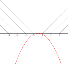
(a)                                               (b)

Figure 7. The decomposition of $\mathcal{B}(\Phi_{2},\Lambda)(t\omega)$.

Let us now study the recurrence relations that the distributions $\mathcal{A}(\Phi,\Lambda,\mathfrak{a},\beta)$ satisfy. It will be convenient to define $\mathcal{A}(\Phi,\Lambda,\mathfrak{a},\beta)$ for any affine subspace $\mathfrak{a}$, by declaring it to be equal to zero if $\mathfrak{a}$ is not admissible. If $\mathfrak{a}=\lambda+\mathfrak{s}$ where $\phi\in\mathfrak{s}$, we denote by $\mathfrak{a}/<\phi>$ the image of the rational space $\mathfrak{a}$ in $V_{0}=V/<\phi>$.

Lemma 9.7.

Let $\phi\in\Phi$ and $\beta\in V$. We still denote by $\beta$ the projection of $\beta$ on $V/<\phi>$.

$(i)$ If $\phi\notin\mathfrak{s}$, then

$$\partial_{\phi}{\mathcal{A}}(\Phi,\Lambda,\mathfrak{a},\beta)={\mathcal{A}}(\Phi\setminus\{\phi\},\Lambda,\mathfrak{a},\beta).$$

$(ii)$ If $\phi\in\mathfrak{s}$, then

$$\partial_{\phi}{\mathcal{A}}(\Phi,\Lambda,\mathfrak{a},\beta)={\mathcal{A}}(\Phi\setminus\{\phi\},\Lambda,\mathfrak{a},\beta)-{\mathcal{A}}(\Phi/<\phi>,\Lambda/<\phi>,\mathfrak{a}/<\phi>,\beta).$$

In $(ii)$, ${\mathcal{A}}(\Phi\setminus\{\phi\},\Lambda,\mathfrak{a},\beta)$ is zero when $\Phi\cap\mathfrak{s}\setminus\{\phi\}$ does not generate $\mathfrak{s}$.

Proof.

Part $(i)$ follows from the relation

$$\partial_{\phi}T(\Phi\setminus\mathfrak{s},\beta_{1})=T((\Phi\setminus\{\phi\})\setminus\mathfrak{s},\beta_{1}).$$

For part $(ii)$ we use equation (3.1.1) on $\tau$, which gives

$$\partial_{\phi}\operatorname{Ber}(\Phi\cap\mathfrak{s},\Lambda\cap\mathfrak{s},\tau)=\operatorname{Ber}((\Phi\cap\mathfrak{s})\setminus\{\phi\},\Lambda\cap\mathfrak{s},\tau)-\operatorname{Ber}(\Phi\cap\mathfrak{s}/<\phi>,\Lambda\cap\mathfrak{s}/<\phi>,\tau).$$

Now suppose $q$ is a polynomial function on $\mathfrak{s}$ constant in the direction of $\phi$. Let $X:=[v_{1},v_{2},\ldots,v_{N}]$ be a sequence of nonzero vectors in $V\setminus\mathfrak{s}$ generating a pointed cone. We denote the projection of $v_{i}$ to $V/<\phi>$ by $\bar{v}_{i}$. Then,

$$\begin{array}[]{ll}q*T(X)(v)&=\displaystyle\int_{0}^{\infty}\cdots\int_{0}^{\infty}q(v-\sum t_{i}v_{i})dt_{1}\cdots dt_{N}\\ &=\displaystyle\int_{0}^{\infty}\cdots\int_{0}^{\infty}q(\overline{v}-\sum t_{i}\bar{v_{i}})dt_{1}\cdots dt_{N}\\ &=\displaystyle q*T(X/<\phi>)(\overline{v}).\end{array}$$

Putting $q=\operatorname{Ber}(\Phi\cap\mathfrak{s}/<\phi>,\Lambda\cap\mathfrak{s}/<\phi>,\tau)$ and $X=\Phi\setminus\mathfrak{s}$, we get part $(ii)$. ∎

Proof.

We now prove Theorem 9.3 by induction on the number of elements in $\Phi$. We assume that the theorem is true for any sublist of $\Phi$. Denote by ${\rm Req}(\Phi)$ the right hand side and by ${\rm Leq}(\Phi)$ the left hand side of equation (9.3.1).

Let $\phi\in\Phi$. Let $\Phi^{\prime}=\Phi\setminus\{\phi\}$. We recall equation (3.1.1),

$$\partial_{\phi}\mathcal{B}(\Phi,\Lambda)=\mathcal{B}(\Phi^{\prime},\Lambda)-\mathcal{B}(\Phi/<\phi>,\Lambda/<\phi>).$$

Let ${\mathcal{R}}_{\rm aff}(\Phi)$ be the collection of all $\Phi$-admissible affine subspaces of $V$. Let ${\mathcal{R}}^{0}$ be the subset consisting of the elements $\mathfrak{a}$ whose direction $\mathfrak{s}$ contains $\phi$.

We now differentiate ${\rm Req}(\Phi)$ with respect to $\phi$. Using relations given in part $(i)$ and $(ii)$ of Lemma 9.7, we get

$$\partial_{\phi}{\rm Req}(\Phi)=\sum_{\mathfrak{a}\in{\mathcal{R}}_{\rm aff}(\Phi)}{\mathcal{A}}(\Phi^{\prime},\Lambda,\mathfrak{a},\beta)-\sum_{\mathfrak{a}\in{\mathcal{R}}^{0}}{\mathcal{A}}(\Phi/<\phi>,\Lambda/<\phi>,\mathfrak{a}/<\phi>,\beta).$$

We observe that the collection of $\mathfrak{a}/<\phi>$ with $\mathfrak{a}\in{\mathcal{R}}^{0}$ parametrizes all affine spaces admissible for $\Phi/<\phi>$. The collection ${\mathcal{R}}_{\rm aff}(\Phi)$ may be larger than ${\mathcal{R}}_{\rm aff}(\Phi^{\prime})$, but, if $\mathfrak{a}$ is not in ${\mathcal{R}}_{\rm aff}(\Phi^{\prime})$, then the contribution ${\mathcal{A}}(\Phi^{\prime},\Lambda,\mathfrak{a},\beta)$ is equal to $0$.

Hence, we obtain by induction that $\partial_{\phi}({\rm Leq}(\Phi)-{\rm Req}(\Phi))=0$ for any $\phi$.

Thus ${\rm Leq}(\Phi)-{\rm Req}(\Phi)$ is constant. But by construction ${\rm Leq}(\Phi)-{\rm Req}(\Phi)$ is equal to zero on $\tau$, therefore the constant is zero. ∎

Example 9.8.

We will give a decomposition formula for the system in Example 2.3. We recall the data: $\Lambda={\mathbb{Z}}e_{1}\oplus{\mathbb{Z}}e_{2}$, $\Phi=[e_{1},e_{2},e_{1}+e_{2}]$.

We will compute $\mathcal{B}(\Phi,\Lambda)(v)$ using the decomposition formula for $v$ in the tope defined by the inequalities $0<v_{2}<1$, $1<v_{1}<2$ and $v_{1}-v_{2}>1$ (see figure 8).

We aim to demonstrate the dependence of the summands in the decomposition formula in Theorem 9.3 to the chosen generic point in a tope, though the value of $\mathcal{B}(\Phi,\Lambda)(v)$ is clearly independent of this choice. We will thus decompose $\mathcal{B}(\Phi,\Lambda)(v)$ in two different ways, for two different choices of generic points lying in the same tope.

Figure 8. Decomposition for various generic points

For the first (resp. second) computation we choose a generic $\beta=b_{1}e_{1}+b_{2}e_{2}$ (resp. $\beta^{\prime}$) in the tope defined by $0<b_{1}<1$, $0<b_{2}<1$ and $b_{1}>b_{2}$, and further satisfying $b_{1}+b_{2}<1$ (resp. $b_{1}+b_{2}>1$).

Figure 8 depicts two such choice of generic elements. We denote the projection of $\beta$ and $\beta^{\prime}$ to $-e_{2}\oplus{\mathbb{R}}(e_{1}+e_{2})$ by $\beta_{0}$ and $\beta_{0}^{\prime}$ respectively. Since these projections lie in different topes for the reduced system $(\Phi\cap\mathfrak{s},\Lambda\cap\mathfrak{s})$ their corresponding contribution to the sum in Theorem 9.3 will be different. In fact, choosing $\beta$ as the generic point will enforce a nonzero contribution of the lattice point $(1,0)$ in evaluating the distribution at a point $v$ as depicted in Figure 8.

Computation with generic point $\beta$:

$$\begin{array}[]{ll}\mathcal{B}(\Phi,\Lambda)(v)=&{\mathcal{A}}(\Phi,\Lambda,V,\beta)(v)+{\mathcal{A}}(\Phi,\Lambda,{\mathbb{R}}e_{2}+e_{1},\beta)(v)\\ &+{\mathcal{A}}(\Phi,\Lambda,{\mathbb{R}}(e_{1}+e_{2})-e_{2},\beta)(v)+{\mathcal{A}}(\Phi,\Lambda,\{(1,0)\},\beta)(v).\end{array}$$

We now compute each summand using the formula in Lemma 7.3.

$$\begin{array}[]{ll}{\mathcal{A}}(\Phi,\Lambda,{\mathbb{R}}e_{2}+e_{1},\beta)(v)&=\operatorname{Ber}(e_{2},\tau(\beta_{0}))*T(\{e_{1},e_{1}+e_{2}\},\beta_{1})(v)\\ &=\delta_{(1,0)}*\operatorname{Res}_{z=0}\left(\left((1/2-\partial{x_{2}})\cdot\frac{e^{\langle v,x+ze^{1}\rangle}}{(x_{1}+z)(x_{1}+x_{2}+z)}\right)_{x=0}\right)\\ &=\frac{1}{2}(v_{1}-1)(-2v_{2}+v_{1})\end{array}$$

$$\begin{array}[]{ll}{\mathcal{A}}(\Phi,\Lambda,{\mathbb{R}}(e_{1}+e_{2})-e_{2},\beta)(v)&=\operatorname{Ber}(e_{1}+e_{2},\tau(\beta_{0}))*T(\{e_{1},e_{2}\},\beta_{1})(v)\\ &=\delta_{(0,-1)}*-\operatorname{Res}_{z=0}\left(\left((1/2-\partial{x_{1}})\cdot\frac{e^{\langle v,x+z(-e^{1}+e^{2})\rangle}}{(x_{1}-x_{2}-z)(x_{2}+z)}\right)_{x=0}\right)\\ &=-\frac{1}{2}(-v_{1}-v_{2})(v_{1}-v_{2}-1)\end{array}$$

$$\begin{array}[]{ll}{\mathcal{A}}(\Phi,\Lambda,\{(1,0)\},\beta)(v)&=\delta_{(1,0)}*-T(e_{1},-e_{2},e_{1}+e_{2})=-(v_{1}-1-v_{2})\end{array}$$

Using the computation in example 2.3 for ${\mathcal{A}}(\Phi,\Lambda,V,\beta)(v)$, we get

$$\begin{array}[]{lll}\mathcal{B}(\Phi,\Lambda)(v)&=&-\frac{1}{6}(v_{1}-2v_{2})(v_{1}-1+v_{2})(2v_{1}-1-v_{2})+\frac{1}{2}(v_{1}-1)(-2v_{2}+v_{1})\\ &&+\frac{1}{2}(v_{1}+v_{2})(v_{1}-v_{2}-1)-(v_{1}-1-v_{2})\\ &=&-\frac{1}{6}(v_{1}-1-2v_{2})(2v_{1}-3-v_{2})(v_{1}-2+v_{2})\end{array}$$

Computation with generic point $\beta^{\prime}$:

$$\begin{array}[]{ll}\mathcal{B}(\Phi,\Lambda)(v)=&{\mathcal{A}}(\Phi,\Lambda,V,\beta^{\prime})(v)+{\mathcal{A}}(\Phi,\Lambda,{\mathbb{R}}e_{2}+e_{1},\beta^{\prime})(v)+\\ &{\mathcal{A}}(\Phi,\Lambda,{\mathbb{R}}(e_{1}+e_{2})+e_{1},\beta^{\prime})(v).\end{array}$$

The first two summands in the decomposition above are already computed. The third summand equals:

$${\mathcal{A}}(\Phi,\Lambda,{\mathbb{R}}(e_{1}+e_{2})+e_{1},\beta^{\prime})(v)=-\frac{1}{2}(2-v_{1}-v_{2})(v_{1}-1-v_{2}).$$

We then have

$$\begin{array}[]{lll}\mathcal{B}(\Phi,\Lambda)(v)&=&-\frac{1}{6}(v_{1}-2v_{2})(v_{1}-1+v_{2})(2v_{1}-1-v_{2})+\frac{1}{2}(v_{1}-1)(-2v_{2}+v_{1})\\ &&-\frac{1}{2}(2-v_{1}-v_{2})(v_{1}-1-v_{2})\\ &=&-\frac{1}{6}(v_{1}-1-2v_{2})(2v_{1}-3-v_{2})(v_{1}-2+v_{2})\end{array}$$

as expected.

In the affine case, we define

$${\mathcal{A}}(\tilde{\Phi},\Lambda,\mathfrak{a},\tau,u)=\operatorname{Ber}(\tilde{\Phi}\cap\mathfrak{s},\tau)*T(\tilde{\Phi}\setminus\mathfrak{s},u).$$

We have a decomposition formula analogous to Theorem 9.3.

Theorem 9.9.

Choose $\beta\in V$ sufficiently generic. Then we have

$$\mathcal{B}(\tilde{\Phi},\Lambda)=\sum_{\mathfrak{a}}{\mathcal{A}}(\tilde{\Phi},\Lambda,\mathfrak{a},\beta).$$

The proof is precisely in the same line of arguments with that of Theorem 9.3.

References

[1]Boysal A. and Vergne M.,Paradan’s wall crossing formula for partitions functions and
Khovanski-Pukhlikov differential operator.
Annales de l’Institut Fourier 59 (2009), 1715-1752.
[2]Brion M. and Vergne M.,Arrangement of hyperplanes I: Rational functions and Jeffrey-Kirwan residue.
Ann. scient. Éc. Norm. Sup. 32 (1999), 715-741.
[3]Brion M. and Vergne M.,Arrangement of hyperplanes II: The Szenes formula and Eisenstein series.
Duke Math. J. 103 (2000), 279–302.
[4]Dahmen and Micchelli,Translates of multivariate splines. Linear Algebra Appl. 52 (1983), 217–234.
[5]De Concini C. and Procesi C.,Topics in hyperplane arrangements, polytopes and
box splines. To appear (available on the personal web page of C. Procesi).
[6]De Concini C., Procesi C. and Vergne M.,
Partition functions and generalized Dahmen-Micchelli spaces. arXiv : math/0805.2907. Transformation
Groups 15 (2010) no 4 , 751-773.
[7]Guillemin V, Lerman E. and Sternberg S.,Symplectic fibrations and multiplicity diagrams.
Cambridge University Press 1996.
[8]Jeffrey, L.C. and Kirwan, F.C., Intersection theory on moduli spaces of holomorphic bundles of arbitrary
rank on a Riemann surface. Ann. of Math. (2) 148 (1998), no. 1, 109–196.
[9]Paradan P-E.,Wall-crossing formulas in Hamiltonian geometry.
arXiv:math/0411306
[10]Paradan P-E.,The moment map and equivariant cohomology with generalized coefficients.
Topology 39 (2001), 401–444.
[11]Paradan P-E.,Localization of the Riemann-Roch character. J. Funct. Anal. 187 (2001), 442–509.
[12]Szenes A.,Iterated Residues and Multiple Bernoulli Polynomials.
International Mathematics Research Notices 18, (1998),
937–956.
[13]Szenes A.,Residue theorem for rational trigonometric sums and Verlinde’s formula.
Duke Math. J. 118 (2003), 189–227.
[14]Szenes A. and Vergne M.,Residue formulae for vector partitions and Euler-MacLaurin sums. Advances in Applied
Mathematics 30 (2003), 295–342.
[15]Szenes A. and Vergne M., and Kostant partition functions arXiv:math/1006.4149.
[16]Vergne M.A Remark on the Convolution with Box Splines. arXiv: math/1003.1574 (to appear in Annals of Mathematics).
[17]Witten E.,On quantum gauge theories in two dimensions. Commun. Math. Phys. 141 (1991), 153–209.