Scaling properties in deep inelastic scattering

Abstract:

We study the scaling properties in deep inelastic scattering using the most recent combined structure function data $F_{2}$ from the H1 and ZEUS collaborations. We also perform a direct fit to the $F_{2}$ data inspired by the scaling properties. Our analysis favours the QCD saturation mechanism from the Balitski Kovchegiv equation wuth running coupling.

1 Scalings in deep inelastic scattering

Geometric scaling [1, 2] is a remarkable empirical property found originally using the data on high energy deep inelastic scattering (DIS) $i.e.$ virtual photon-proton cross-sections. One can represent with reasonable accuracy the cross section $\sigma^{\gamma^{*}p}$ by the formula $\sigma^{\gamma^{*}p}(Y,Q)=\sigma^{\gamma^{*}}(\tau)\ ,$ where $Q$ is the virtuality of the photon, $Y$ the total rapidity in the ${\gamma^{*}}$-proton system and

$$\tau=\log Q^{2}-\log Q_{s}(Y)=\log Q^{2}-\lambda Y\ ,$$ (1)

is the scaling variable. A fit to the DIS data measured leads to a value of $\lambda\sim.3$, which confirms the value found within the Golec-Biernat and Wüsthoff model [3] where geometric scaling was explicitely used for the parametrization.

The scaling using the variable $\tau$ defined in Formula 1 is directly related to the concept of saturation, the behaviour of perturbative QCD amplitudes when the density of partons becomes high enough. There were many theoretical arguments to infer that in a domain in $Y$ and $Q^{2}$ where saturation effects set in, geometric scaling is expected to occur. Within this framework, the function $Q_{s}(Y)$ can be called the saturation scale, since it determines the approximate upper bound of the saturation domain.

This type of geometric scaling is motivated by asymptotic properties of QCD evolution equations with rapidity. Using the nonlinear Balitsky-Kovchegov (BK) equation [4] which represents the “mean-field” approximation of high energy (or high density) QCD, geometric scaling could be derived from its asymptotic solutions [5]. This equation is supposed to capture some essential features of saturation effects. Considering the BK equation with $fixed$ coupling constant leads asymptotically to the original geometric scaling of Formula 1. Considering a $running$ coupling leads to the following scaling

$$\tau=\log Q^{2}-\log Q_{s}(Y)=\log Q^{2}-\lambda\sqrt{Y}\ ,$$ (2)

Recently [6], it was noticed that the scaling solution 2 of the BK equation with running coupling is only approximate and not unique. Another equivalent approximation leads to a different scaling variable, namely

$$\tau=\log Q^{2}-\lambda~{}\frac{Y}{\log Q^{2}}\ .$$ (3)

The effect of QCD fluctuations was examined in Ref. [7] in the fixed coupling scheme and gives rise to a new “diffusive scaling”, the scaling variable being

$$\tau=\frac{\log Q^{2}-\lambda{Y}}{\sqrt{Y}}\ .$$ (4)

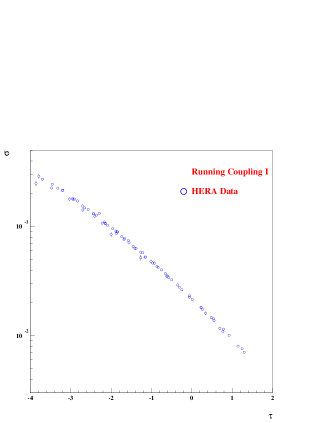
Figure 1: DIS cross section data as a function of the scaling variable for Running Coupling I.

The aim of this study from a theoretical point-of-view is to test and compare the different scaling behaviors, arising from different versions of QCD evolution, using the most recent precise data available from HERA resulting from a combination of the H1 and ZEUS $F_{2}$ measurements [8]. We study the quality of the description of these combined data set using the four kinds of scaling and refer to them in the following as “Fixed Coupling” for the variable 1, “Running Coupling I” and “Running Coupling II” for the variables 2 and 3 respectively, and to “Diffusive Scaling” for 4.

2 The Quality Factor

In order to compare the quality of the different scalings and to check if the DIS cross sections $\sim F_{2}/Q^{2}$ depend mainly on the $\tau$ variable or not, it is useful to introduce the concept of Quality Factor [9] (QF) while the explicit form of the $\tau$ dependence is not known. After normalising the data sets $v_{i}=\log(\sigma_{i})$ and scalings $u_{i}=\tau_{i}(\lambda)$ between 0 and 1, and ordering the scalings in $u_{i}$, we define QF

$$QF(\lambda)=\left[\sum_{i}\frac{(v_{i}-v_{i-1})^{2}}{(u_{i}-u_{i-1})^{2}+\epsilon^{2}}\right]^{-1}.$$

$\epsilon$ is needed in the case that two data points have the same scaling, namely when they have the same $x$ and $Q^{2}$, and we take $\epsilon$=0.01. The method is to fit the value of $\lambda$ to maximize QF.

3 Scaling tests in DIS

As we mentioned, we use the very precise data sets combining the H1 and ZEUS measurements of the proton structure function $F_{2}$ [8]. To remain in the region where perturbative QCD is applicable and to avoid the region where valence quarks dominate, we choose to restrict ourselves to data points with $4\leq Q^{2}\leq 150$ GeV² and $x\leq 10^{-2}$. In addition, in order to avoid the high $y$ region where $F_{L}$ is large, we add an additional cut on data on $y\leq 0.6$. After all cuts, we are left with 117 data points.

The values of the $\lambda$ parameters and the QF are given in Table I for the different scaling considered in this analysis. While Fixed Coupling, Running Coupling I and II lead to approximately the sames value of QF, Diffusive Scaling is clearly disfavoured. As an example, the scaling plot showing all combined DIS cross section data as a function of the $\tau$ variable for Running Coupling I is given in Fig. I to show the quality of scaling. In addition, it is worth noticing that adding additional variables such as $Q_{0}$ or a shift in rapidity $Y_{0}$ does not improve the scaling quality.

scaling	parameter	1/QF
Fixed Coupling	$\lambda=0.31$	150.2
Running Coupling I	$\lambda=1.61$	137.9
Running Coupling II	$\lambda=2.76$	124.3
Diffusive Scaling	$\lambda=0.31$	210.7

Table 1: Values of $1/QF$ and of the $\lambda$ parameter for the four different kinds of scaling considered

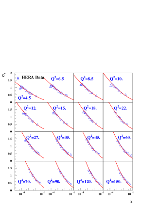
Figure 2: Result of the Running Coupling I fit to the combined $F_{2}$ data set from H1 and ZEUS. We note a fair description of data for $x\leq 10^{-2}$ and $y\leq 0.6$.

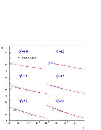
Figure 3: Extrapolation of the Running Coupling I fit to the combined $F_{2}$ data set from H1 and ZEUS at low $Q^{2}$ values.

4 Fits to HERA data

In this section, we describe a fit to the combined HERA data motivated by the success of the data description using the Running Coupling I scaling variable. In the fit, we will use all data above $Q^{2}=4GeV^{2}$ since the fitting formula that we develop is valid only in the dilute regime, and saturation is supposed to occur at very low $Q^{2}$ at HERA. The following formula, deduced from the dipole amplitude with saturation including the asymptotic expression of the Airy function which is the solution of the Balistsky-Kovchegov equation, is used to fit the data

$$\tau = \log(\frac{Q^{2}}{Q_{0}^{2}})-\lambda\sqrt{\log(\frac{1}{x})-Y_{0}}$$

$$\sigma = N\exp(-\alpha\tau)\exp\left(\frac{-\beta\tau^{3/2}}{(\log{1/x}-Y_{0})^{1/4}}\right)$$

where the different parameters used in the fit are $\lambda$, $\alpha$, $\beta$, $Q_{0}$, $Y_{0}$ and $N$. We notice that this formula shows only a moderate scaling violation introduced by the $(\log{1/x}-Y_{0})^{1/4}$ term predicted by the dipole model and we perform the fits with and without this term.

The fit results and the parameter values are given in Table II and Fig. II. We note that the fit $\chi^{2}$ is close to 1.2 per dof and is similar with or without the scaling violation term. The fit cannot describe the reduction of the reduced cross section at high $y$ due to the large values of $F_{L}$. In Fig. III, we also show the fit extrapolation at lower $Q^{2}$ which leads to a fair description of data. Going to lower values of $Q^{2}$ will require a parametrisation valid in the saturated region whereas our formula is only valid in the dilute regime.

In addition, we also attempted to perform a similar fit inspired by Fixed Coupling or Running Coupling II, but they lead to a worse description of data ($\chi^{2}=$156.4 and 190.4 respectively).

Parameter	Fit I	Fit II
$\lambda$	1.54 $\pm$ 0.02	1.54 $\pm$ 0.02
$\alpha$	0.34 $\pm$ 0.01	0.18 $\pm$ 0.01
$\beta$	0.24 $\pm$ 0.01	0.18 $\pm$ 0.01
$Q_{0}$	0.079 $\pm$ 0.01	0.064 $\pm$ 0.01
$Y_{0}$	-1.46 $\pm$ 0.02	0.50 $\pm$ 0.02
$N$	0.51 $\pm$ 0,01	0.72 $\pm$ 0,01
$\chi^{2}$	130.1	119.0

Table 2: Value of the parameters of the Running Coupling I inspired fit to the combined DIS cross section 117 data points from HERA. Fit I (resp. Fit II) is performed with (resp. without) the scaling violation term.

5 Conclusion

In this paper, we presented a new study of scaling properties in DIS using the most recent combined $F_{2}$ data from H1 and ZEUS. The new precise data set shows precise scaling using either Fixed Coupling, Running Coupling I or II, while Diffusive Scaling is disfavoured. A direct fit inspired by Running Coupling I leads to a good description of data in the dilute regime.

References

- [1] A. M. Staśto, K. Golec-Biernat, and J. Kwiecinski, Phys. Rev. Lett. 86, 596 (2001).
- [2] G. Beuf, R. Peschanski, C. Royon, D. Salek, Phys. Rev. D78, 074004 (2008).
- [3] K. Golec-Biernat and M. Wusthoff, Phys. Rev. D 59, 014017 (1999).
- [4] I. Balitsky, Nucl. Phys. B 463, 99 (1996); Y. V. Kovchegov, Phys. Rev. D 60, 034008 (1999), D 61, 074018 (2000).
- [5] S. Munier and R. Peschanski, Phys. Rev. Lett. 91, 232001 (2003), Phys. Rev. D69, 034008 (2004), D 70, 077503 (2004).
- [6] G. Beuf, preprint arXiv:0803.2167.
- [7] Y. Hatta, E. Iancu, C. Marquet, G. Soyez and D. N. Triantafyllopoulos, Nucl. Phys. A 773, 95 (2006) [arXiv:hep-ph/0601150].
- [8] F. D. Aron et al., H1 and ZEUS collaborations, JHEP 1001 (2010) 109.
- [9] F. Gelis, R. Peschanski, G. Soyez and L. Schoeffel, Phys. Lett. B 647, 376 (2007) [arXiv:hep-ph/0610435].