Multi-shocks in asymmetric simple exclusions processes: Insights from fixed-point analysis of the boundary-layers

Abstract

The boundary-induced phase transitions in an asymmetric simple exclusion process with inter-particle repulsion and bulk non-conservation are analyzed through the fixed points of the boundary layers. This system is known to have phases in which particle density profiles have different kinds of shocks. We show how this boundary-layer fixed-point method allows us to gain physical insights on the nature of the phases and also to obtain several quantitative results on the density profiles especially on the nature of the boundary-layers and shocks.

I Introduction

Asymmetric simple exclusion process (ASEP) is a non-equilibrium process in which particles hop to the neighboring site in a specific direction following certain conditions ligett . In the simplest model, particles obey the mutual exclusion condition due to which a site cannot be occupied by more than one particle and a hop to the neighboring site is possible provided this target site is empty. The particles after being injected at one end of the lattice at a rate $\alpha$ hop across the lattice and reach the other end where they are withdrawn at a rate $1-\gamma$. There exist other models where particles can have attractive or repulsive interaction in addition to the exclusion interaction kls ; hager .

All these systems exhibit interesting boundary-induced phase transitions for which the tuning parameters are the boundary rates, $\alpha$ and $\gamma$ krug ; straley . In different phases, the average particle density has distinct constant values across the bulk of the lattice. These particle density profiles in different phases may also differ due to different location and nature of the boundary-layers. More features, such as coexistence of high and low-density regimes are seen in systems where particle number is not conserved in the bulk due to attachment and detachment of particles to and from the lattice parameg ; smsmb . In this coexistence phase (also known as a shock phase), the particle density profile has a jump discontinuity (shock) in the interior of the lattice from a low to a high density value. The slope and the number of such shocks in a density profile are related to the nature of the inter-particle interactions which determine the fundamental current density relation sm ; rakos . Although this relation predicts the kind of shocks that can be seen rakos in the density profile, a systematic characterization of the phase-transition and the phase diagram in the $\alpha-\gamma$ plane requires a detailed analysis of the relevant equations describing the dynamics in the steady-state smb ; smsmb ; jaya . Drawing analogies from the equilibrium phase transitions, first order, critical straley ; parameg and tricritical jaya kind of phase transitions have been observed so far in various ASEP models.

While characterizing the phase transitions, it is useful to study the variation of the height or the width of the boundary-layers as $\alpha$ and $\gamma$ are changed. In a way, these boundary-layers play important roles in deciding the ”order parameter” like quantities in these non-equilibrium phase transitions. Owing to their importance in describing phase transitions, the boundary-layers for several interacting and non-interacting models have been studied using the techniques of boundary-layer analysis cole . It is found that the system usually enters into a shock phase from a non-shock phase due to the deconfinement of the boundary-layer from the boundary. This deconfinement can be described by a nontrivial scaling exponent associated with the width of the boundary-layer smsmb . For the pure exclusion case, except for a critical point, the transition from a non-shock to a shock phase is first order in nature since a shock of finite height is formed on the phase boundary. The height of the shock on the phase boundary reduces as one approaches the critical point along the phase boundary. At the critical point, the shock height is zero on the phase boundary and it increases continuously as one proceeds away from the phase-boundary further into the shock phase. In order to visualize these features, it is beneficial to obtain the full solution for the density profile along with its boundary-layer. Boundary layer analysis is useful for this purpose since it allows us to generate a uniform approximation for solving the steady-state particle density equation across the entire lattice. This steady-state equation can be obtained from the large time- and length-scale limit (hydrodynamic limit) of the statistically averaged master equation that describes the particle dynamics in the discrete form. For the simple exclusion case, it is possible to obtain an analytical solution of the steady-state hydrodynamic equation for the entire density profile. This, however, may not possible for more complex ASEPs.

A fixed-point analysis of the hydrodynamic equation turns smfixedpt out to be general and useful, since it does not involve an explicit solution of the steady-state hydrodynamic equation. In particle conserving models, a boundary-layer saturates to the constant bulk density profile asymptotically. As a consequence of this, it is expected that the fixed-points of the boundary-layer equation match with the bulk density values. In other words, a boundary-layer, which is a solution of the boundary-layer equation, is a part of the flow trajectory of the equation flowing to the appropriate fixed-point on the phase plane. Thus, in order to find out the values of the bulk-densities in different phases, it is sufficient to determine the physically acceptable fixed-points of the boundary-layer equation. As a result, the number of possible bulk phases is given by the number of these fixed-points. Applying this method to a specific particle conserving two-species ASEP smfixedpt , it is found that this system has three distinct bulk phases corresponding to three fixed-points of the boundary-layer equations. In addition, it is possible to predict the nature of phase transitions, locations of the boundary-layers etc. for this system. All these predictions match well with the results from numerical simulations popkov .

In a particle non-conserving case, the density is not constant in the bulk, and therefore, the fixed-points of the boundary-layer do not provide the full profile since the details of the bulk dynamics is not considered in this approach. However, it is still useful to obtain the fixed-points of the boundary-layer equations along with their stability properties in order to predict the possible shapes of the density profiles under different boundary conditions. In the present paper, we consider a particle number non-conserving model where particles interact repulsively. Our aim is to extend the fixed-point analysis to a system with non-constant bulk density. We show how this analysis helps us predict possible shapes of the density profiles under different boundary conditions and also understand the properties of different kinds of shocks present in the density profile. This particular model is chosen because of certain nontrivial shapes of the density profiles with different kinds of shocks.

The plan of the paper is as follows. In the following section, we describe the model. This section also contains brief discussions on the hydrodynamic approach, boundary-layer analysis and some of the known results. In section III, we present the phase-plane analysis of the boundary-layer equations for the present model. There are separate subsections on the boundary-layer equation, its fixed-points, stability analysis of the fixed-points and possible shapes of shocks. Section IV presents the predictions of the possible shapes of the density profile under different boundary conditions. In section V, we mention a few general rules for predicting the shapes of the density profiles and some special features related to the shocks of this model. We end the paper with a summary in section VI.

II Model

II.1 Discrete description

The asymmetric simple exclusion process that we consider here consists of a one-dimensional lattice of $N$ sites with lattice spacing, $a$. Particles are injected at $i=1$ with rate $\alpha$ and withdrawn at $i=N$ at a rate $1-\gamma$. Particles, obeying mutual exclusion, hop to the right with rates that depend on the occupancy of the neighboring site as

$$1100\rightarrow 1010\ \ {\rm at}\ \ {\rm a}\ \ {\rm rate}\ \ 1+\epsilon,$$ (1)

$$0101\rightarrow 0011\ \ {\rm at}\ \ {\rm a}\ \ {\rm rate}\ \ 1-\epsilon,$$ (2)

$$0100\rightarrow 0010\ \ {\rm at}\ \ {\rm rate}\ \ 1$$ (3)

$$1101\rightarrow 1010\ \ {\rm at}\ \ {\rm rate}\ \ 1.$$ (4)

Here, $0<\epsilon<1$ and $1$ ($0$) represents an occupied (unoccupied) site. For $\epsilon\neq 0$, there is an effective repulsion between the particles kls ; hager ; rakos . In addition, the number of particles is not conserved due to particle detachment, $1\rightarrow 0$, at a rate $\omega_{d}$ and attachment, $0\rightarrow 1$, at a rate $\omega_{a}$ at any site on the lattice. Particle attachment and detachment are equilibrium like processes that do not give rise to any particle current.

II.2 Hydrodynamic Approach and a brief description of the boundary-layer analysis

The hydrodynamic approach is based on the lattice continuity equation which equates the time evolution of the particle occupancy at a given site with the difference of currents across its two neighboring bonds. In the continuum description, the continuous time and space variables are $t$ and $x$ with the latter replacing, for example, the $i$th site as $i\rightarrow x=ia$. Upon doing a Taylor expansion of the statistically averaged continuum version of the lattice continuity equation in small $a$, one has the following hydrodynamic equation

$$\frac{\partial\rho}{\partial t}+\frac{\partial J}{\partial x}+S_{0}=0,$$ (5)

for the averaged particle density $\rho(x,t)$. This equation has already been supplemented with the particle non-conserving parts

$$S_{0}=-\Omega(\rho_{L}-\rho),$$ (6)

where $\rho_{L}=\frac{\omega_{a}}{\omega_{a}+\omega_{d}}$ and $\Omega=(\omega_{a}+\omega_{d})N$. The current, $J(\rho)$, consists of a bulk current $j(\rho)$ and a diffusive current proportional to $\frac{\partial\rho}{\partial x}$ as

$$J=-\epsilon_{0}\frac{\partial\rho}{\partial x}+j(\rho).$$ (7)

Here, $\epsilon_{0}$ is a small parameter proportional to $a$. The diffusive current part arises naturally as one retains terms up to $O(a^{2})$ in the Taylor expansion. In order to determine the particle density, $\rho(x)$, in the steady-state ($\frac{\partial\rho}{\partial t}=0$), one has to solve the differential equation with appropriate boundary conditions. We consider the lattice-ends to be attached to the particle-reservoirs which maintain constant densities $\rho(x=0)=\alpha$ and $\rho(x=1)=\gamma$. The diffusive current part is crucial here since due to its presence, the hydrodynamic equation becomes a second order differential equation and as a result we can obtain a smooth solution satisfying both the boundary conditions.

$\epsilon=0$ is the usual ASEP with only the exclusion interaction. In this case, the current density relation, $j(\rho)=\rho(1-\rho)$ is an exact one. The symmetric shape of the current about its maximum at $\rho=1/2$ is a consequence of its invariance under particle-hole exchange $\rho\rightarrow 1-\rho$. It is well understood that the phase diagram has low-density ($\rho<1/2$ at the bulk), high-density ($\rho>1/2$ at the bulk) and maximum current ($\rho=1/2$ at the bulk) phases straley . The particle-hole symmetry is retained in $\epsilon\neq 0$ models although the current changes non-trivially. At $\epsilon=1$, i.e. for the extreme repulsion case, hops such as $0101\rightarrow 0011$ are forbidden. The current, therefore, vanishes exactly at the half-filling ($\rho=1/2$) with the maximum current appearing symmetrically for densities on the two sides of $\rho=1/2$. The exact form of the current as a function of $\rho$ for arbitrary $\epsilon$ can be found using a transfer matrix approach hager and it evolves from a single to a symmetric double peak structure as $\epsilon$ grows beyond $\epsilon_{J}\approx.8$. A simple, analytically tractable form of the current with double peaks can be obtained by doing a double expansion of the exact current about $\epsilon=\epsilon_{J}$ and $\rho=1/2$ jaya . This leads to a quadratic form for the current

$$j(\rho)=(2r+u)/16-\frac{r}{2}(\rho-1/2)^{2}-u(\rho-1/2)^{4},$$ (8)

where the constant term is chosen in such a way that $j(\rho)=0$ for $\rho=0,\ {\rm or}\ 1$. We recover the non-interacting limit, $j(\rho)=\rho(1-\rho)$ for $r=2$ and $u=0$. The double peak shape appears for $r<0$. In the entire analysis below, we consider $r$ to be a small negative parameter and $u>0$.

For the boundary-layer analysis, it is important to consider the bulk part and the narrow boundary-layer or the shock regions of the density profile separately. These boundary-layers or shocks are formed over a narrow region of width $O(\epsilon_{0})$ and they merge to the bulk density in the appropriate asymptotic limit. In order to study the boundary-layer and its asymptotic approach to the bulk, one can rescale the position variable in (5) as $\tilde{x}=(x-x_{0})/\epsilon_{0}$, where $x_{0}$ is the location of the center of the boundary-layer. Hence, for a boundary-layer satisfying the boundary condition at $x=1$, we have $x_{0}\approx 1$. For small $\epsilon_{0}$, the boundary-layer approaches the bulk density in the $\tilde{x}\rightarrow-\infty$ limit and satisfies the boundary condition at $\tilde{x}=0$. In terms of $\tilde{x}$, the steady-state hydrodynamic equation is

$$\frac{\partial^{2}\rho}{\partial\tilde{x}^{2}}-\frac{\partial j}{\partial\tilde{x}}-\epsilon_{0}S_{0}=0.$$ (9)

Since $\epsilon_{0}$ is a small parameter, the effect of the particle non-conserving term, $S_{0}$, on the boundary-layer is negligible. As a result the total current, $J=j(\rho)-\frac{\partial\rho}{\partial\tilde{x}}$ is constant across the boundary-layer. A shock, therefore, can be represented by a horizontal line connecting two densities in the $j-\rho$ plane as shown in figure (1).

Figure 1: Current $j$ is plotted as a function of $\rho$. Lines ’a’ and ’b’ represent an upward and a downward shock respectively.

For an upward shock ($\frac{\partial\rho}{\partial\tilde{x}}>0$), this line lies below the $j(\rho)$ curve and the reverse is true for a downward shock ($\frac{\partial\rho}{\partial\tilde{x}}<0$). As a result, while for $r>0$, only upward shocks are possible, for $r<0$, there can be density profiles with a downward shock and double shocks. Double shocks can be represented by two horizontal lines on the $j-\rho$ plane below the two peaks in $j(\rho)$.

To zeroth order in $\epsilon_{0}$, the final boundary-layer equation is

$$\frac{\partial^{2}\rho}{\partial\tilde{x}^{2}}-\frac{\partial j}{\partial\tilde{x}}=0.$$ (10)

In the boundary-layer language, the solution of this equation is known as the inner solution. To obtain the bulk part of the density profile, one can ignore the diffusive current part in $J$ for small $\epsilon_{0}$. The steady-state equation that gives the bulk part of the density profile is

$$\frac{dj}{dx}+S_{0}=0.$$ (11)

The solution of this equation for the bulk part of the profile is known as the outer solution. These inner and outer solutions contain several integration constants which are fixed by the boundary conditions and other matching conditions of the boundary-layer and the bulk under various limits. Since the slope of the outer solution is obtained from

$$\frac{d\rho}{dx}=-S_{0}/\frac{dj}{d\rho},$$ (12)

for a given $\rho$, the slope depends crucially on the signs of $(\rho_{L}-\rho)$ and $\frac{dj}{d\rho}$. For all the analysis below, we consider $\rho_{L}$ to be large and $\alpha$ and $\gamma$ to be much smaller than $\rho_{L}$.

II.3 Known results

Double peak structure of the current-density relation leads to two maximum current and one minimum current phases in the phase diagram of the particle conserving repulsion model hager . In the maximum and minimum current phases, the bulk density values are those at which the current attains its maximum and minimum values respectively. With these new phases, the phase diagram for this model becomes more complex than its non-interacting counterpart.

Combining the techniques of boundary-layer analysis and the results from numerical solutions, the phase diagram has been obtained for the particle non-conserving repulsion model jaya . The phase diagram has a lot of interesting features including a tricritical point at $r=0$. In the $\alpha-\gamma-r$ phase diagram, this is a special point where two critical lines meet. It has been found that three different phase diagrams are possible for $r>0$, $r=0$ and $r<0$. For $r>0$, the current-density plot is symmetric around $\rho=1/2$ with a maximum at $\rho=1/2$. The nature of the phase diagram is qualitatively similar to the mutually exclusive case with one single critical point. For $r<0$, with a double peak structure of the current-density plot, the phase diagram is more complex with more than one critical point and three different shock phases with the density profile having a single upward shock, double upward shocks and one upward and one downward shock jaya ; rakos .

The low-density peak can give rise to a low-density upward shock ($\rho(x)\leq 1/2$ in the shock part) in the density profile. A single shock of this kind can be represented by a horizontal line in the $j-\rho$ plane below the low-density peak. The critical point corresponds to a situation where the horizontal line reaches the peak position implying a shock of zero height. The second distinct critical point that involves both the peaks of the current-density plot is not symmetrically related to this. The density profile, here, has two upward shocks, in which one is a low-density shock and one is a high-density shock with $\rho>1/2$. The low-density shock, in this case, has the maximum height with its high-density end saturating to $\rho=1/2$. The high-density shock which is due to the high-density peak of the current-density plot can be of varying height. The critical point corresponds to the special point where this high-density shock has zero height. In addition to these regions, there are regions in the phase diagram, where density profiles with a downward shock or a single, symmetric upward shock are found.

In view of the symmetry of the $j-\rho$ diagram, it is natural to expect the two critical points to be related through this symmetry. Previous work, however, shows that the shapes of the density profiles are not related through this symmetry near these two special points. Unlike the low-density shock, the high-density shock in the density profile is always accompanied by a low-density shock of maximum height. The following analysis clearly reveals the reasons behind such asymmetries.

III Phase-plane analysis of the boundary-layer equations

In the following subsections, we determine the fixed-points of the boundary-layer equation and their stability properties. These fixed-points are the special points to which the boundary-layer solution saturates in the appropriate limit. The knowledge about the fixed-points and their stabilities can, therefore, be used to our advantage to find out, for example, the bulk densities to which a shock or a boundary-layer saturates at its two edges.

III.1 Boundary-layer equation

Substituting the expression for $j(\rho)$ as given in (8) and integrating the boundary-layer equation, (10) once, we have

$$\frac{d\rho_{1}}{d\tilde{x}}+\frac{r}{4}\rho_{1}^{2}+\frac{u}{8}\rho_{1}^{4}=C_{0}.$$ (13)

Here $\rho_{1}=2\rho-1$ and $C_{0}$ is the integration constant. The saturation of the boundary-layer to the bulk density, $\rho_{1b}$, is ensured by choosing the integration constant as

$$C_{0}=\frac{r}{4}\rho_{1b}^{2}+\frac{u}{8}\rho_{1b}^{4}.$$ (14)

As per equation (8), $C_{0}$ is related to the excess current (positive, negative or zero) measured from $\rho=1/2$ (half-filled case). The entire analysis in the following is done in terms of $\rho_{1}$ for which the boundary conditions are $\rho_{1}(x=0)=\alpha_{1}=2\alpha-1$ and $\rho_{1}(x=1)=\gamma_{1}=2\gamma-1$.

III.2 fixed-points

$C_{0}$ can be plotted for various $\rho_{1b}$ varying from $-1$ to $1$. For $r<0$, $C_{0}$ has a symmetric double well structure around $\rho_{1b}=0$ (see figure (2)).

Figure 2: $C_{0}$ plotted as a function of $\rho_{1b}$ with $r=-.2$ and $u=2.2$

The fixed-points, $\rho_{1}^{*}$, of equation (13), are the solutions of the algebraic equation

$$\frac{u}{8}\rho_{1}^{4}+\frac{r}{4}\rho_{1}^{2}-C_{0}=0.$$ (15)

In general, there are four possible solutions for the fixed-point as

$$\rho_{1}^{*}=\pm[\frac{\mid r\mid\pm\sqrt{r^{2}+8C_{0}u}}{u}]^{1/2}.$$ (16)

The value of $C_{0}$ depends on $\rho_{1b}$, the bulk density to which the boundary-layer solution saturates. As a consequence, for a given $C_{0}$, the corresponding $\rho_{1b}$ is always a fixed-point. For the same $C_{0}$, there are, however, other fixed-points which are determined from (16). Hence, from the information about one saturation density $\rho_{1b}$, the other saturation density of the shock can always be determined. The approach to various fixed-points has to be, of course, consistent with their stability properties. These stability properties of various fixed-points are discussed in the following subsection.

If $C_{0}$ is positive, there can be only two real fixed-points of opposite signs. The positive and negative fixed-points denoted respectively as $\rho_{1\pm}^{*}$ are

$$\rho_{1\pm}^{*}=\pm[\frac{\mid r\mid+\sqrt{r^{2}+8C_{0}u}}{u}]^{1/2}.$$ (17)

If $C_{0}<0$, there are four fixed-points for $\rho_{1b}$. In all these cases, the fixed-points are symmetrically located on the either side of the origin. The positive $\rho_{1}$ fixed-points are

$$\rho_{1,2+}^{*}=[\frac{\mid r\mid\pm\sqrt{r^{2}-8\mid C_{0}\mid u}}{u}]^{1/2}$$ (18)

and the negative $\rho_{1}$ fixed-points are

$$\rho_{1,2-}^{*}=-[\frac{\mid r\mid\pm\sqrt{r^{2}-8\mid C_{0}\mid u}}{u}]^{1/2}.$$ (19)

Here, the subscripts $1$ and $2$ correspond to the $+$ and $-$ signs inside the square bracket respectively. It is important to notice that for $C_{0}<0$, all the fixed-points become imaginary when $\mid C_{0}\mid>\frac{r^{2}}{8u}$. As $C_{0}$ approaches this lowest negative value, the pair of fixed-points on the positive and negative sides approach each other and they merge at $C_{0}=-\frac{\mid r\mid^{2}}{8u}$. At this special value, the fixed-points are $\rho_{1m}^{*\pm}=\pm(\frac{\mid r\mid}{u})^{1/2}$. For $C_{0}=0$, there are three fixed-points, $\rho_{1}^{*}=0$ and $\rho_{10}^{*\pm}=\pm(\frac{2\mid r\mid}{u})^{1/2}$.

Numerical values of the fixed-points for some special values of $C_{0}$ with $r=-.2$ and $u=2.2$ are mentioned below. For $C_{0}=0$, the nonzero fixed-points are $\rho_{10}^{*\pm}=0,\ \ \pm.426$. For these values of $r$ and $u$, no real fixed-points are present if $C_{0}<-\frac{r^{2}}{8u}=-.00227$. At this special value of $C_{0}$, the two fixed-points are $\rho_{1m}^{*\pm}=\pm.30151$.

III.3 Stability analysis of the fixed-points

For $C_{0}>0$, a linearization of equation (13) around the fixed-points with $\rho_{1}=\rho_{1}^{*}+\delta\rho_{1}$ leads to the following stability equation

$$\frac{d\delta\rho_{1}}{d\tilde{x}}=\frac{-\sqrt{\mid r\mid^{2}+8uC_{0}}}{2}\rho_{1}^{*}\delta\rho_{1}.$$ (20)

This implies that the fixed-points $\rho_{1+}^{*}$ and $\rho_{1-}^{*}$ are, respectively, stable and unstable.

Similarly, for $C_{0}<0$, the general stability equation is

$$\frac{d\delta\rho_{1}}{d\tilde{x}}=\frac{\rho_{1}^{*}}{2}\ \delta\rho_{1}({\mid r\mid}-{u}{\rho_{1}^{*}}^{2}).$$ (21)

The flow around the fixed-points can be obtained by substituting the explicit expressions of the fixed-points. Figure (3) shows the stability properties of various fixed-points for $C_{0}>0$ and $C_{0}<0$.

Figure 3: flow behavior of the fixed-points

The stability property of the $\rho_{1}^{*}=0$ fixed-point for $C_{0}=0$ and for the pair of fixed-points for $C_{0}=-\frac{r^{2}}{8u}$ cannot be determined from the linear analysis. However, the flow around the fixed-points can be predicted from the continuity of the flow behavior as $C_{0}$ approaches these special values. Fixed-points, their stability properties and how the fixed-points change with $C_{0}$ are combinedly shown in figure (4).

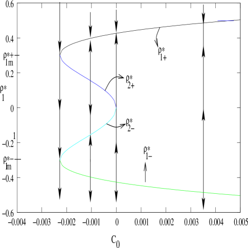
Figure 4: Fixed-points are plotted for different values of $C_{0}$ with $r=-.2$ and $u=2.2$. $\rho_{1\pm}^{*}$ and $\rho_{2\pm}^{*}$ are different fixed-points as mentioned in the text. The vertical solid lines with arrows show the flow behavior of the fixed-points.

III.4 Shocks for various $C_{0}$

Since $C_{0}$ can be expressed purely in terms of $J$, with its constant parts subtracted, it remains constant across a shock or a boundary-layer. In principle, using equation (14), one can obtain the value of $C_{0}$ along the continuously varying parts of the density profile. Hence, as we move along a density profile having bulk shocks, $C_{0}$ changes as per equation (14) along the outer solution parts of the profile with intermediate constant values across the shock or inner solution regions. The value of $C_{0}$ in the shock region is fixed by one of the bulk density values to which the shock saturates.

With the information on the possible values of $C_{0}$ in the entire range of $\rho_{1b}$ and, hence, the knowledge about the corresponding fixed-points, it is possible to list the kind of shocks that can be observed.

Let us assume that the shocks or the boundary-layers approach the bulk densities $\rho_{1r}$ or $\rho_{1l}$ as $\tilde{x}\rightarrow\pm\infty$ respectively. Since $\rho_{1l}$ and $\rho_{1r}$ are various fixed-points of the inner equation, the approach to these fixed-points has to be consistent with the flow properties. A shock is called an upward shock if $\rho_{1l}<\rho_{1r}$. The reverse i.e. $\rho_{1l}>\rho_{1r}$ is true for a downward shock.

(i) $C_{0}>0$: In this case, there are two fixed-points $\rho_{1+}^{*}$ and $\rho_{1-}^{*}$ symmetrically located around $\rho_{1}=0$ with $\rho_{1-}^{*}$ being an unstable fixed-point. Thus if a shock is formed with $C_{0}>0$, it should be an upward shock which approaches the fixed-points $\rho_{1r}=\rho_{1+}^{*}$ and $\rho_{1l}=\rho_{1-}^{*}$ as $\tilde{x}\rightarrow\infty$ and $-\infty$ respectively. The shock height, in this case, is $\rho_{1+}^{*}-\rho_{1-}^{*}$.

(ii) $C_{0}<0$: In this case, four fixed-points lead to different kinds of shocks.

(a) It is possible to see a downward shock with $\rho_{1l}=\rho_{2+}^{*}$ and $\rho_{1r}=\rho_{2-}^{*}$. The downward shock is thus symmetric around $\rho_{1}=0$. The flow in figure (3) shows that a downward shock cannot involve other fixed-points since that would not be consistent with the stability criteria of the fixed-points.

(b) There can be small upward shocks which lie entirely in the range $\rho_{1}>0$. We have already referred these shocks as high-density shocks. In terms of the fixed-points, the left and right saturation densities of the shock are $\rho_{1l}=\rho_{2+}^{*}$ and $\rho_{1r}=\rho_{1+}^{*}$, respectively.

(c) The third possibility is that of an upward shock entirely in $\rho_{1}\leq 0$ range. Such a shock has been referred as a low-density shock. For this shock, $\rho_{1l}=\rho_{1-}^{*}$ and $\rho_{1r}=\rho_{2-}^{*}$.

(iii) $C_{0}=0$: There can be an upward shock with $\rho_{1r}=0$ and $\rho_{1l}=\rho_{1-}^{*}$. There can also be an upward shock connecting the densities $\rho_{1l}=0$ and $\rho_{1r}=\rho_{1+}^{*}$. These two shocks together appear as a large shock, symmetric around $\rho_{1}=0$.

Alternatively, different kinds of shocks can tell us the range of values for $C_{0}$.

IV Predictions about the shapes of the density profiles

Based on figure (4), we attempt to predict possible shapes of the density profiles for given boundary conditions $\alpha_{1}$ and $\gamma_{1}$. We consider only a few pairs of boundary conditions and based on this, we make certain general predictions in the next section. The basic strategy for drawing the density profile is as follows. We first need to mark $\alpha_{1}$ and $\gamma_{1}$ on the $\rho_{1}^{*}$ axis of $C_{0}-\rho_{1}^{*}$ plane. Starting with either of the boundary conditions, we change $\rho_{1}$, along the curve in figure (4), in a way that we reach the other boundary condition in the end of our move. While doing so, we may allow a discontinuous variation of $\rho_{1}$ along a vertical constant-$C_{0}$ line, provided it does not violate the flow property. Such a discontinuous change in $\rho_{1}$ appears in the form of a shock or a boundary-layer in the density profile. The dashed, vertical lines in figure (5a), for example, are the constant-$C_{0}$ lines along which the density may change. Such a dashed-line, therefore, represents a boundary-layer or a shock in the density profile. Two densities at which a shock or a boundary-layer saturates, are those at which a particular, constant-$C_{0}$ line, representing a shock or a boundary-layer, intersects the curves. This method, however, sometimes leaves us with different options for the density profile. All these possibilities are shown on $C_{0}-\rho_{1}^{*}$ plane for each pair of boundary conditions individually.

(a)

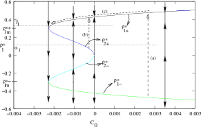
(b)

Figure 5: (a) Possible variations of the density, as one moves along the density profile from $x=0$ end, are shown on the $C_{0}-\rho_{1}^{*}$ plane. Bold dashed lines or curves with open arrows show the variation of the density. Open arrows point in the direction of increasing $x$. Dotted lines mark the boundary conditions $\alpha_{1}$ and $\gamma_{1}$. Solid lines with arrows are the flow trajectories of the fixed-points. (b) Numerical solutions for the density $\rho_{1}$ for various $\alpha_{1}$ with $\gamma_{1}=0.34$. The inset gives a zoomed view of the particle-depleted boundary-layer at $x=0$. No boundary-layer is formed near $x=1$.

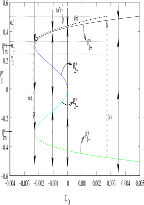
(a) (b)

(c)

Figure 6: (a) Same captions as figure (5a) except that here we explicitly show possible density variations for two different left boundary conditions specified by $\alpha_{1}$ and $\alpha_{1}^{\prime}$. (b) Numerical solutions for $\rho_{1}(x)$ for various $\alpha_{1}$ with $\gamma_{1}=0.23$. The main figure provides a zoomed view of the boundary-layers near $x=0$. The entire density profile over the entire lattice is shown in the inset. (c) A zoomed view of the same density profiles near the $x=1$. This shows the particle depleted boundary-layers near $x=1$.

IV.1 Density profiles with only boundary-layers

Suppose we consider a situation where $\alpha_{1},\ \gamma_{1}>0$ with $\alpha_{1}<\rho_{1m}^{*+}$ and $\gamma_{1}>\rho_{1m}^{*+}$. There can be a possibility where the density profile has a particle-depleted boundary-layer ($\frac{d\rho_{1}}{dx}\mid_{x=0}>0$) at $x=0$ satisfying the boundary conditions $\rho_{1}(x=0)=\alpha_{1}$. This boundary-layer can be represented by a vertical line similar to (a) in figure (5a). This is consistent with the flow property that suggests the approach of the boundary-layer to the fixed-point $\rho_{1+}^{*}$ as $\tilde{x}\rightarrow\infty$. On the other hand, in the $\tilde{x}\rightarrow-\infty$ limit, which corresponds to the unphysical negative $x$ region, the boundary-layer saturates to the unstable fixed-point $\rho_{1-}^{*}$. After the boundary-layer, the density may decrease continuously along (c) on the $\rho_{1+}^{*}$ branch and satisfies the boundary condition, $\rho_{1}(x=1)=\gamma_{1}$. There can be another possibility where the particle-depleted boundary-layer at $x=0$ is represented by a vertical line similar to (b) joining the fixed-points $\rho_{2+}^{*}$ and $\rho_{1+}^{*}$. The boundary condition at $x=1$ is again satisfied by a decreasing density part parallel to (c). For this to be possible the condition $\gamma_{1}<\rho_{10}^{*+}$ is required. These two possibilities are distinct due to distinctly different values of $C_{0}$. This shows the crucial role played by $C_{0}$ in deciding the density profile. Numerical solutions of the full steady-state hydrodynamic equation presented in figure (5b) show the boundary-layers saturating to a bulk density $\rho_{1b}\approx.48$. This implies that the boundary-layers are indeed represented by (a) type vertical lines.

(a)

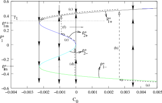
(b)

Figure 7: (a) This figure has the same caption as figure (4). (b) Plot of the density profiles $\rho_{1}(x)$ for various large negative values of $\alpha_{1}$ with $\gamma_{1}=.32$. No boundary-layer is formed at $x=0$ or $x=1$. A few density profiles towards right have double shocks.

(2) Next, we consider $\alpha_{1},\gamma_{1}>0$ with $\alpha_{1}>\rho_{1m}^{*+}$ and $\gamma_{1}<\rho_{1m}^{*+}$. In this case too, the density profile can satisfy the boundary condition at $x=0$ through a boundary-layer that can be represented by a line similar to (a) in figure (6a). This would be a particle depleted boundary-layer at $x=0$. In order to satisfy the other boundary condition, the density should decrease till $\rho_{1m}^{*+}$ along path (b) on the $\rho_{1+}^{*}$ branch and then satisfy the right boundary condition through a particle-depleted boundary-layer along (c) in figure (6a). The boundary condition at $x=0$ can also be satisfied by vertical lines coming from above the $\rho_{1+}^{*}$ branch leading to particle-rich boundary-layers ($\frac{d\rho_{1}}{dx}\mid_{x=0}<0$) at $x=0$. These lines could be (a’) type lines in figure (6a) satisfying the boundary condition $\alpha_{1}^{\prime}$. Both particle-depleted and particle-rich boundary-layers are present in the density profiles of figure (6b) obtained by solving the full steady-state hydrodynamic equation numerically.

IV.2 Density profiles with upward shocks

With $\gamma_{1}>\rho_{1m}^{*+}$ and $\alpha_{1}$ large negative, possible shapes of the density profile can be of the following kinds. We start with $\rho_{1}(x=0)=\alpha_{1}$. $\rho_{1}$ decreases continuously along $\rho_{1-}^{*}$ branch along the dashed line (a) in figure (7a). After this part, an upward shock, represented by a vertical line similar to either (b) or (d) appears. In the latter case, the dashed line (a) should be extended further till it reaches the low-density end of (d). If the shock is represented by (b), it is a large shock, symmetric around $\rho_{1}=0$. In the second case, the shock is a low-density shock with the saturation densities being $\rho_{1r}=0$ and $\rho_{1l}=\rho_{10}^{*-}$. If the density approaches the $\rho_{1+}^{*}$ branch after the large shock, the boundary condition at $x=1$ can be satisfied after that by a decrease in density along (c) on this branch. If the shock is of (d) kind, the density has to change further to satisfy the right boundary condition. Upon reaching $\rho_{1}=0$ value, the density may change along $\rho_{2-}^{*}$ or the $\rho_{2+}^{*}$ branch. The flow around $\rho_{1}^{*}=0$, however, suggests that the density variation only along $\rho_{2+}^{*}$ branch (path (e) in the figure (7)) is possible. The continuously increasing part along (e) is then followed by another upward shock, given by line (f), taking the density to $\rho_{1+}^{*}$ branch. The boundary condition is then satisfied by a continuously decreasing part along a (c) type line. Numerical solutions in figure (7b) are consistent with these predictions.

IV.3 Density profiles with downward shocks

We next consider a case $\rho_{1m}^{*-}<\gamma_{1}<0$ with $\alpha_{1}$ increasing from large negative values. Here we specifically mention how the density profile changes as $\alpha_{1}$ is changed keeping $\gamma_{1}$ fixed. In the process, we observe how a density profile with a downward shock appears. Let us assume that our starting $\alpha_{1}$ lies somewhere on the $\rho_{1-}^{*}$ branch. $\rho_{1}$ increases from $\rho_{1}(x=0)=\alpha_{1}$ along $\rho_{1-}^{*}$ branch till it reaches the boundary $x=1$. This continuously increasing part is represented by (1a) in figure (8a). The density, then, satisfies the right boundary condition through a boundary-layer which can be, for example, represented by a vertical line like (1b), in figure (8a). This line takes the solution from the unstable fixed-point $\rho_{1-}^{*}$ to the stable fixed-point $\rho_{1+}^{*}$. Since the vertical line (1b) passes through $\gamma_{1}$ before reaching the $\rho_{1+}^{*}$ branch, the boundary-layer satisfies the boundary condition before saturating to the positive fixed-point, $\rho_{1+}^{*}$. The boundary-layer at $x=1$ is, therefore, a part of this vertical, constant-$C_{0}$ line.

(a)

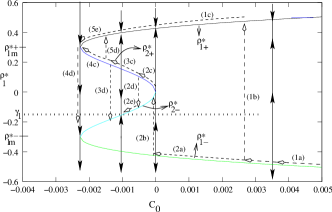
(b)

(c)

Figure 8: (a) The trajectory of the density on $C_{0}-\rho_{1}$ plane. Five possible trajectories are shown. These trajectories are distinguished by different numbers. Alphabetical sequence represents the variation of the density along increasing $x$. (b) Plot of the density profiles $\rho_{1}(x)$ for various $\alpha_{1}$ with $\gamma_{1}=-.28$. (c) Zoomed views of the of the boundary-layers of the density profiles in (a) near $x=1$.

As $\alpha_{1}$ is increased slightly, the route of the density along $\rho_{1-}^{*}$ branch remains the same but this time the density reaches a higher value than the previous $\alpha_{1}$ case before increasing sharply as a boundary-layer satisfying the boundary condition at $x=1$. As $\alpha_{1}$ is increased further, for a given $\alpha_{1}$, the continuously increasing part of the profile reaches the low-density end of the line (2b). After this, there is a shock in the density profile of (2b) kind. This is a low-density shock that takes the density to $\rho_{1}^{*}=0$. If this jump is near the boundary, this shock becomes actually a boundary-layer that can help the density satisfy the boundary condition at $x=1$. However, if this discontinuity is in the bulk, it is an upward low-density shock. In case of a shock in the bulk, the density increases further along $\rho_{2+}^{*}$ branch (path (2c) in figure (8)). The boundary condition, however, demands a decrease in $\rho_{1}$. This is possible through a downward vertical line (similar to path (2d)) and then a continuously decreasing part (2e) along $\rho_{2-}^{*}$ branch. The path (2d) is a downward shock that is seen in figure (8b) and (8 c). In case the density varies along lines (3c) and (3d), we have a downward boundary-layer near $x=1$. These possibilities are expected if $\alpha_{1}$ is increased further from its value that leads to (2c) and (2d) type variations. As before, the principle is that if the (3d) type vertical line intersects $\gamma_{1}$ line before reaching the $\rho_{2-}^{*}$ branch, (3d) type line represents a boundary-layer satisfying the boundary condition at $x=1$. If the reverse happens, this downward vertical line represents a downward shock at the bulk which needs to be followed by a continuously decreasing density part along the $\rho_{2-}^{*}$ branch. This is a general principle which can be applied to other cases also to see the deconfinement of a boundary-layer giving rise to a shock in the bulk (see reference smsmb ).

With further increase of $\alpha_{1}$, the density variation from from $x=0$ end, is still the same as before up to part (3c) along the $\rho_{2+}^{*}$ curve except that now the density approaches closer to $\rho_{1m}^{*+}$ along (4c) like path. Finally for a given $\alpha_{1}$, the density reaches the value $\rho_{1m}^{*+}$. After this, the boundary condition is satisfied through a depleted boundary-layer represented by vertical path (4d). With further increase of $\alpha_{1}$, the density cannot now go around $\rho_{1m}^{*+}$ to move to $\rho_{1+}^{*}$ branch due to the constraint from the stability property. In that case, the only option for the density is to proceed along (4c) but move to $\rho_{1+}^{*}$ branch along a vertical line similar to (5d) before reaching the point $\rho_{1m}^{*+}$. There is now a second high-density upward shock in the density profile at larger $x$ (line (5d)) with the first shock being a low-density one represented by the line, (2b). With the increase of $\alpha_{1}$, the (5d) type vertical line moves to higher values of $C_{0}$. The boundary condition at $x=1$ is now satisfied by the rest of the density profile where the density decreases continuously along (5e) path to the minimum $\rho_{1m}^{*+}$ and after that decreases through a depleted boundary-layer represented by the line (4d). Thus, for example, for this value of $\alpha_{1}$, we see the following parts in the density profile as we move along the density profile from its $x=0$ end. (i) A continuously varying density profile that satisfies the boundary condition $\rho(x=0)=\alpha_{1}$. (ii) This is followed by a low-density upward shock of maximum height connecting $\rho_{1l}=\rho_{10}^{*-}$ and $\rho_{1r}=0$. (iii) Beyond this shock, there is again a continuously increasing part. (iv) This is followed by an upward, high-density shock. (v) Beyond this high-density shock, the density decreases continuously to $\rho_{1m}^{*+}$. (vi) The last part is a particle-depleted boundary layer, that saturates to $\rho_{1m}^{*+}$ for $x<1$ and satisfies the boundary condition at $\rho_{1}(x=1)=\gamma_{1}$. All these features can be verified from the density profile in figure (8a).

If $\alpha_{1}$ is increased further, the upward high-density shock (vertical lines like (5d)) will move towards higher $C_{0}$ values. For certain $\alpha_{1}$, the low and the high-density shocks merge and there is a big symmetric shock with $C_{0}=0$. Beyond this $\alpha_{1}$, the big upward shock still persists and this is followed by a continuously varying part (similar to (1c)) along which the density decreases and approaches $\rho_{1m}^{*+}$. The boundary condition is again satisfied by the particle-depleted boundary-layer represented by (4d).

V General predictions

Since the boundary-layers or shocks are the special features through which the density profiles are distinguished, our general predictions are more on the kind of shocks or boundary-layers that can be seen under various boundary conditions.

V.1 Shocks and boundary-layers

Downward shock in the bulk or a particle-depleted boundary-layer at $x=1$: Either of these features appears whenever the density profile decreases through a jump discontinuity from the $\rho_{2+}^{*}$ branch to the $\rho_{2-}^{*}$ branch or from $\rho_{1m}^{*+}$ to $\rho_{1m}^{*-}$. The condition for this is $\gamma_{1}<\rho_{1m}^{*+}$. The value of $\alpha_{1}$ is somewhat flexible since it is possible to see these features both for $\alpha_{1}$ positive or negative.

Upward symmetric shock in the bulk or depleted boundary-layer at $x=0$: This is seen whenever the density profile jumps from $\rho_{1-}^{*}$ to $\rho_{1+}^{*}$. This happens for various combinations of $\alpha_{1}$ and $\gamma_{1}$ such as $\alpha_{1}<0$ or $\alpha_{1}>0$ with $\gamma_{1}>\rho_{1m}^{*+}$ or $\gamma_{1}<\rho_{1m}^{*+}$. At $x=0$, the density profile may start with a continuously varying part followed by a symmetric large shock, or it can satisfy the boundary condition at $x=0$ with the help of a boundary-layer. In both cases, the discontinuity in the density corresponds to a discontinuous jump from $\rho_{1-}^{*}$ to $\rho_{1+}^{*}$.

The presence or absence of a boundary-layer at $x=0$ is specified completely by the value of $C_{0}$ at $x=0$. Let us assume that $\rho_{1}=\alpha_{1}$ line intersects the curve on figure (4) at a value $C_{0}=C_{0}(\alpha_{1})$. A condition as $C_{0}(\alpha_{1})=C_{0}(x=0)$, would mean a continuously varying density near $x=0$. If these two values are unequal, it would imply the presence of a boundary-layer. For example, for $\alpha_{1}>\rho_{1m}^{*+}$, a particle-rich or a particle-depleted boundary-layer appears if $C_{0}(\alpha_{1})>C_{0}(x=0)$ and $C_{0}(\alpha_{1})<C_{0}(x=0)$, respectively. However, it is important to pay attention to certain situations which are forbidden due to the stability properties. For example, if $\alpha_{1}<\rho_{1m}^{*-}$ , a boundary-layer with $C_{0}(x=0)<C_{0}(\alpha_{1})$ is not possible.

Double shock: In this case, the density profile has both high and low-density upward shocks with the low-density shock having maximum possible height, $\rho_{10}^{*-}$. In order to have a high-density shock, the lower end of the high-density shock must be on the $\rho_{2+}^{*}$ branch. The density can reach this branch only via $\rho_{1}=0$ point. The only way the density can reach the $\rho_{1}=0$ point is through a low-density shock represented by the $C_{0}=0$ line across the negative lobe. A low-density shock representing a jump across the negative lobe along $C_{0}=0$ line has the maximum possible height.

A density-profile with double shock may appear for $\alpha_{1}<\rho_{1m}^{*-}$ and $\gamma_{1}<\rho_{1m}^{*+}$ or $\gamma_{1}>\rho_{1m}^{*+}$. In case of $\gamma_{1}>\rho_{1m}^{*+}$, the density after the high-density shock varies continuously along $\rho_{1+}^{*}$ branch to satisfy the boundary condition at $x=1$. For $\gamma_{1}<\rho_{1m}^{*+}$, the second shock is possible for some $\alpha_{1}$. In this case, after reaching the $\rho_{1+}^{*}$ branch, the density decreases till $\rho_{1m}^{*+}$ and then decreases further as a depleted boundary-layer at $x=1$ to satisfy the boundary condition.

It is interesting to note that although it is possible to have a profile with only a low-density shock, the same with a single high-density shock is never possible. The flow behavior suggests that a high-density shock has to be always accompanied by a low-density shock of maximum height.

Boundary-layer at $x=1$: As in the case of a boundary-layer at $x=1$, it is also possible to specify the conditions for a boundary-layer at $x=1$ by comparing the value of $C_{0}(x=1)$ with $C_{0}(\gamma_{1})$. In general, a boundary-layer will appear at $x=1$ if these two values of $C_{0}$ are different. As an example, a downward boundary-layer for $\rho_{1m}^{*-}<\gamma_{1}<\rho_{1m}^{*+}$ appears if $C_{0}(x=1)<C_{0}(\gamma_{1})$.

V.2 Saturation of the shock

From equation (13), we find that near the saturation to a bulk density $\rho_{1b}$, the slope of the boundary-layer is given by

$$\frac{d\delta\rho_{1}}{d\tilde{x}}=(\frac{\mid r\mid}{2}-\frac{u}{2}\rho_{1b}^{2})\rho_{1b}\delta\rho_{1}$$ (22)

where it is assumed that the boundary-layer density is $\delta\rho_{1}$ away from the saturation value, $\rho_{1b}$. This shows, that the saturation of the boundary-layer to the bulk is in general exponential except for three special points. The saturation is of power-law kind, if $\rho_{1b}=0$ or $\rho_{1b}=\rho_{1m}^{*\pm}=\pm(\frac{r}{u})^{1/2}$. The length scale associated with the exponential approach of the shock to the bulk density diverges as the bulk density approaches these special values. As discussed in subsection II.3, the critical points, correspond to special boundary conditions $(\alpha_{c},\gamma_{c})$ at which the shock height across the positive or negative lobe reduces to zero. Therefore, the approach to the critical point is associated with the continuous vanishing of the shock height along with the divergence of the length scale over which the shock saturates to the bulk.

VI Summary

Here, we have considered an asymmetric simple exclusion process of interacting particles on a finite, one dimensional lattice. These particles have mutual repulsion in addition to the exclusion interaction. Apart from the hopping dynamics of the particles, the model also has particle attachment-detachment processes, which lead to particle non-conservation in the bulk. Such processes are known to exhibit boundary-induced phase transitions for which the tuning parameters are the boundary densities, $\alpha$ and $\gamma$. In different phases, the average particle density distributions across the lattice have distinct shapes with various types of discontinuous jumps from one density value to another. Here, we carry out a phase-plane analysis for the boundary-layer differential equation to understand how the fixed-points of the boundary-layer equation and their flow properties determine the shape of the entire density profile under given boundary conditions. Such a fixed-point analysis has been extremely useful in understanding the phases and phase transitions of particle conserving models for which the constant bulk density values in different phases are given by the physically acceptable fixed-points of the boundary-layer equation. In addition, the number of steady-state phases, the nature of the phase-transitions, the locations of the boundary-layers can be obtained analytically from the phase-plane analysis of the boundary-layer equation. The present work provides a generalization of the method to a particle non-conserving process.

To apply this method, we have considered the hydrodynamic limit of the statistically averaged master equation describing the particle dynamics. The hydrodynamic equation, describing the time evolution of the average particle density, looks like a continuity equation supplemented with the particle non-conserving terms. The current contains the exactly known hopping current and a regularizing diffusive current part. The boundary-layer equation, which is the main focus of this work, can be obtained from the particle conserving part of the hydrodynamic equation. For convenience, we use $\rho_{1}=2\rho-1$ for the boundary-layer equation. $\rho_{1}$ is related to the deviation from $\rho=1/2$ (half filled case).

It is found that the fixed-points, $\rho_{1}^{*}$, of the boundary-layer equation are determined in terms of a parameter $C_{0}$ related to the excess current measured from $\rho=1/2$ (half-filled case). Since the fixed-points are dependent on $C_{0}$, one can plot the physically acceptable fixed-points as a function of $C_{0}$ on the $C_{0}-\rho_{1}^{*}$ plane. In the steady-state, the constancy of the current across a shock or a boundary-layer implies that such objects can be represented by a fixed value of $C_{0}$. The boundary-layers or shocks of the density profiles are represented by the constant-$C_{0}$ lines on this $C_{0}-\rho_{1}^{*}$ plot. The densities at which the constant-$C_{0}$ line intersects the fixed-point branches are the densities to which the shock or the boundary-layer saturates. The discontinuous change of the density has to be consistent with the stability properties of the fixed-points. For given values of $\alpha$ and $\gamma$, we can start from the $x=0$ end of the density profile and find out how the density can change along the profile as it proceeds to satisfy the boundary condition at $x=1$. This density variation along the density profile can be conveniently marked on the $C_{0}-\rho_{1}^{*}$ plot to see its consistency with the flow properties of the fixed-points. Our approach does not give any information about the location of a shock since it does not involve the details of the bulk part of the profile. Instead, it is found that the conserved quantity, $C_{0}$, plays an important role in deciding the shape of the density profile.

The emphasis of our approach is on the boundary-layer equation which appears to control the shape of the entire density profile. Particle non-conserving processes are not important for the boundary layers. This simplicity allows us not only to classify different kinds of density distributions, but also to gain more physical insight as why some features of the density profile are evident under certain boundary conditions. Some of these features are mentioned in the list below.

(a) When a density profile has two shocks, the low-density shock is of maximum possible height. For given values of the interaction parameters, the height of the low-density shock can be obtained explicitly.

(b) It is possible to have a low-density shock alone in the profile but a high-density shock has to be always accompanied by a low-density shock of maximum height.

(c) A downward shock is produced by the deconfinement of a downward boundary-layer at $x=1$. The condition on $\gamma$ for seeing a downward shock or a downward boundary-layer at $x=1$ can be precisely specified.

(d) The symmetric two peak structure of the current as a function of the particle density is responsible for a symmetric two lobe structure of the fixed-points drawn on $C_{0}-\rho_{1}^{*}$ plane. The flow behavior of the fixed-points around the two lobes are asymmetric. This is the reason why the two critical points in the phase diagram are not symmetrically related to each other. This asymmetry is reflected in the shapes of the density profiles near these critical points.

(e) For a given boundary condition, a density profile with only one boundary-layer and no shock can be fully specified by the value of $C_{0}$ at this end.

In addition to these issues, this analysis also provides quantitative predictions regarding the heights of different kinds of shocks and their approach to the bulk along with the length scale associated with it.

Acknowledgement Financial support from the Department of Science and Technology, India and warm hospitality of ICTP (Italy), where the work was initiated, are gratefully acknowledged.

References

- (1) T. Ligett, Interacting Particle Systems: Contact, Voter and Exclusion Processes (Springer-Verlag, Berlin, 1999).
- (2) S. Katz, J. L. Lebowitz and H. Spohn, J. Stat. Phys. 34, 497 (1984).
- (3) J. S. Hager, J. Krug, V. Popkov and G. M. Schuetz, Phys. Rev. E 63, 056110 (2001).
- (4) J. Krug, Phys. Rev. Lett. 67, 1882 (1991).
- (5) A. B. Kolomeisky, G. M. Schuetz, E. B. Kolomeisky and J. P. Straley, J. Phys. A 31, 6911 (1998).
- (6) A. Parameggiani, T. Franosch and E. Frey, Phys. Rev. E 70, 046101 (2004). M. R. Evans, R. Juhasz and L. Santen, Phys. Rev. E 68, 026117 (2003).
- (7) S. Mukherji and S. M. Bhattacharjee, J. Phys. A 38, L285 (2005); S. Mukherji and V. Mishra, Phys. Rev. E 74, 01116 (2006).
- (8) S. Mukherji, Phys. Rev. E 76, 011127 (2007).
- (9) V. Popkov, A. Rakos, R. D. Willmann, A. B. Kolomeisky and G. M. Schuetz, Phys. Rev. E 67, 066117 (2003).
- (10) S. M. Bhattacharjee, J. Phys.A 40, 1703 (2007).
- (11) J. Maji and S. M Bhattacharjee, Europhysics Letters 81, 30005 (2008).
- (12) J. D. Cole, Perturbation Methods in Applied Mathematics (Blaisdell Publishing, Massachusetts, 1968).
- (13) S. Mukherji, Phys. Rev. E 79, 041140 (2009).
- (14) V. Popkov, J. Stat. Mech. P07003 (2007); V. Popkov and G. M. Schuetz, J. Stat. Mech. P12004 (2004).