Stable topological modes in two-dimensional Ginzburg-Landau models with trapping potentials

Abstract

Complex Ginzburg-Landau (CGL) models of laser media (with the cubic-quintic nonlinearity) do not contain an effective diffusion term, which makes all vortex solitons unstable in these models. Recently, it has been demonstrated that the addition of a two-dimensional periodic potential, which may be induced by a transverse grating in the laser cavity, to the CGL equation stabilizes compound (four-peak) vortices, but the most fundamental “crater-shaped” vortices (CSVs), alias vortex rings, which are, essentially, squeezed into a single cell of the potential, have not been found before in a stable form. In this work we report families of stable compact CSVs with vorticity $S=1$ in the CGL model with the external potential of two different types: an axisymmetric parabolic trap, and the periodic potential. In both cases, we identify stability region for the CSVs and for the fundamental solitons ($S=0$). Those CSVs which are unstable in the axisymmetric potential break up into robust dipoles. All the vortices with $S=2$ are unstable, splitting into tripoles. Stability regions for the dipoles and tripoles are identified too. The periodic potential cannot stabilize CSVs with $S\geq 2$ either; instead, families of stable compact square-shaped quadrupoles are found.

I Introduction

A broad class of pattern-formation models in one- and multi-dimensional geometries is based on the complex Ginzburg-Landau (CGL) equations with the cubic-quintic (CQ) nonlinearity AK ; AA2 . Arguably, these models find the most important realization is lasing media, where the CQ terms account for the combination of nonlinear gain and loss (the CGL equation also includes the linear loss) lasers . In terms of actual laser systems, the CQ nonlinearity represents configurations incorporating the usual linear amplifiers and saturable nonlinear absorbers. In the one-dimensional (1D) setting, the CQ CGL equation readily gives rise to stable solitary pulses (dissipative solitons). These solutions and their physical implications have been studied in numerous works Boris .

A well-known problem is the search for stable dissipative solitons in the two-dimensional (2D) version of CGL equations. In that case, the challenging factors are the possibility of the critical collapse induced by the cubic self-focusing term, and the vulnerability of vortex solitons, which are shaped as vortex rings, to azimuthal perturbations that tend to split them we ; PIO ; splitting . Actually, Petviashvili and Sergeev Petv had originally introduced the CGL equation with the CQ nonlinearity with the purpose to develop a model admitting stable localized 2D patterns. Stable 2D solitary vortices (alias spiral solitons), with topological charge (vorticity) $S=1$ and $2$, were first reported in Ref. Lucian . Stable vortex solitons were reported in the 3D version of the CQ CGL equation too we2

The general form of the CQ CGL equation for the amplitude of the electromagnetic field, $E(x,y,z)$, which propagates along axis $z$ in a uniform bulk medium with transverse coordinates $\left(x,y\right)$, is we2

$$iE_{z}+\left(\frac{1}{2}-i\beta\right)\left(E_{xx}+E_{yy}\right)+i\delta E$$

$$+(1-i\varepsilon)|E|^{2}E+(\nu+i\mu)|E|^{4}E=0,$$ (1)

where $\delta$ is the linear-loss coefficient, the Laplacian with coefficient $1/2$ represents, as usual, the transverse diffraction in the paraxial approximation, $\beta$ is an effective diffusion coefficient, $\varepsilon$ is the cubic gain, the Kerr coefficient is normalized to be $1$, and quintic coefficients $-\nu$ and $\mu$ account for the saturation of the cubic nonlinearity ($\nu>0$ corresponds to the quintic self-focusing, which does not lead to the supercritical collapse, being balanced by the quintic loss Herve_PRA_2009 ).

The physical interpretation of all terms in Eq. (2) is straightforward, except for the diffusion. This term arises in some models of large-aspect-ratio laser cavities, close to the lasing threshold. Actually, such models are based on the complex Swift-Hohenberg equation lega , which reduces to the CGL equation for long-wave excitations. In the usual situation, the diffusion term is artificial in the application to optics. Nevertheless, $\beta>0$ is a necessary condition for the stability of dissipative vortex solitons, while the fundamental ($S=0$) solitons may be stable at $\beta=0$ Lucian ; we2 . Therefore, a challenging problem is to develop a physically relevant modification of the the 2D CGL model, without the diffusivity ($\beta=0$), that can support stable localized vortices. Recently, it has been demonstrated that this problem can be resolved by adding a transverse periodic potential to Eq. (1), which casts the CGL equation into the following form Herve_PRA_2009 :

$$iE_{z}+\frac{1}{2}\left(E_{xx}+E_{yy}\right)+i\delta E+(1-i\varepsilon)|E|^{2}E$$

$$+(\nu+i\mu)|E|^{4}E-V\left(x,y\right)E=0.$$ (2)

The periodic potential can be induced by a grating, i.e., periodic modulation of the local refractive index in the plane of $\left(x,y\right)$ :

$$V(x,y)=p\left[\cos\left(2x\right)+\cos\left(2y\right)\right],~{}p>0\text{,}$$ (3)

where $p$ is proportional to the strength of the underlying grating, and the scaling invariance of of Eq. (2) was employed to fix the period of potential (3) to be $\pi$.

The laser-writing technology makes it possible to fabricate permanent gratings in bulk media Jena . In addition, in photorefractive crystals virtual photonic lattices may be induced by pairs of laser beams illuminating the sample in the directions of $x$ and $y$ in the ordinary polarization, while the probe beam is launched along axis $z$ in the extraordinary polarization Moti-general .

As concerns the physical interpretation of the model, it is relevant to notice that the equations of the CGL type describe laser cavities, where the mode-locked optical signal performs periodic circulations, as a result of averaging fs . Therefore, the transverse grating (or a different structure inducing the effective transverse potential) is not required to fill the entire cavity; a layer localized within a certain segment, $\Delta z$, rather than uniformly distributed along $z$, may be sufficient to induce the effective potential in Eq. (2) Herve_PRA_2009 .

Stationary solutions to Eq. (2) are sought for as $E\left(x,y,z\right)=e^{ikz}U\left(x,y\right)$, with real propagation constant $k$ and complex function $U\left(x,y\right)$ satisfying the stationary equation,

$$\left[-k+i\delta-V\left(x,y\right)\right]U+\frac{1}{2}\left(U_{xx}+U_{yy}\right)$$

$$+\left(1-i\varepsilon\right)\left|U\right|^{2}U+\left(\nu+i\mu\right)\left|U\right|^{4}U=0.$$

Stable vortices, supported by periodic potential (3), were constructed in Ref. Herve_PRA_2009 as compound objects, built of four separate peaks of the local power, which are set in four cells of the lattice. Two basic types of such vortices are “rhombuses”, alias onsite vortices, with a nearly empty cell surrounded by the four filled ones BBB , and “squares”, alias offsite vortices, which feature a densely packed set of four filled cells Yang . The vorticity (topological charge) of these patterns is provided by phase shifts of $\pi/2$ between adjacent peaks, which corresponds to the total phase circulation of $2\pi$ around the pattern, as it should be in the case of vorticity $S=1$. In the experiment, stable compound vortices with $S=1$ were created in a conservative medium, viz., the above-mentioned photorefractive crystals with the photoinduced lattice MotiYuri . In Ref. Herve_PRA_2009 , a stability region was identified for rhombus-shaped compound vortices, with $S=1$, in the framework of the CGL equation (2) with potential (3), and examples of their stable square-shaped counterparts (which are essentially less stable than the rhombuses) were produced too. In addition, Ref. Herve_PRA_2009 reported examples of stable rhombic quadrupoles, i.e., four-peak patterns with alternating signs of the peaks (and zero vorticity).

A challenging issue remains to find conditions providing for the stability of compact “crater-shaped” vortices (CSVs, alias vortex rings) which, unlike the compound vortical structures, are squeezed into a single cell of the periodic potential (typical examples of stable “craters” supported by 2D periodic potentials can be seen below in Fig. 13). These nearly axisymmetric vortices are most similar to their counterparts found in the free space Lucian . As mentioned above, in the absence of the potential the vortices may only be stabilized by the diffusion term in Eq. (1), with $\beta>0$; otherwise, azimuthal perturbations break them into sets of fragments. A natural expectation is that the trapping potential may stabilize “craters” in the model with $\beta=0$. Nevertheless, no examples of stable CSVs were reported in Ref. Herve_PRA_2009 .

The search for stable CSVs is also a challenging problem in the studies of 2D conservative models with lattice potentials. In particular, only unstable vortices of this type were reported in the 2D nonlinear Schrödinger (NLS) equation with the CQ nonlinearity and a checkerboard potential Radik1 ; Radik2 (see also Ref. Arik ). On the other hand, stable supervortices, i.e., chains formed by compact craters with $S=+1$ and an independent global vorticity, $S^{\prime}=\pm 1$, imprinted onto the chain, were found as stable objects in 2D NLS equations with periodic potentials and the cubic or CQ nonlinearities supervortex ; Radik2 . Eventually, a stability region for CSVs was recently identified in the cubic NLS equation, provided that the periodic potential is strong enough super-stable .

The main objective of the present work is to demonstrate that crater-shaped dissipative vortex solitons may be stabilized, in the framework of the CQ CGL equation (2), by external potentials. To this end, we consider two potentials: the periodic one, taken as per Eq. (3), and also the axisymmetric trapping potential,

$$V\left(x,y\right)=\left(\Omega^{2}/2\right)r^{2},$$ (4)

where $r^{2}\equiv x^{2}+y^{2}$. The consideration of potential (4) is suggested by known results for the 2D NLS equation (in that context, it is introduced as the Gross-Pitaevskii equation for the Bose-Einstein condensate), which demonstrate that potential (4) can stabilize localized vortices with $S=1$ against the splitting GPE . Actually, potential (4) can be realized in the laser cavity merely by inserting a lens with focal length $f^{\prime}=k/(L\Omega^{2})$, where $k$ is the wavenumber and $L$ the cavity length. Then, averaging over the cyclic optical path yields potential (4), within the framework of the paraxial approximation. It is possible to check that the generic situation for vortices and other types of dissipative solitons generated by Eq. (2) may be adequately represented by fixing $\delta=1/2$, $\mu=1$, and $\nu=-0.1$, which is assumed below. Two remaining parameters, that will be varied in this work, play a crucially important role in the model: cubic gain $\varepsilon$ and the strengths, $\Omega^{2}$ or $p$, of the trapping potentials.

The rest of the paper is organized as follows. In Sections 2 and 3, we consider the stabilization of the CSVs in axisymmetric potential (4). First, we apply the generalized variational approximation (VA), which was developed in Ref. Vladimir for a class of CGL equations, as an extension of the well-known VA for conservative nonlinear-wave systems Progress . In Section 3 we continue the consideration of the CSVs in the same potential by means of numerical methods. Both the VA and direct simulations reveal the existence of a broad stability region for these vortices with $S=1$. Unstable CSVs split into stable patterns in the form of dipoles. Vortices with $S=2$ can also be constructed, but they all are unstable (similar to the situation in the NLS equation GPE ), splitting into tripole patterns. Dipoles and tripoles are studied in Section 4, where their stability regions are identified.

A stability region for CSVs with $S=1$ in periodic potential (3) is reported in Section 5. This is a novel result, as stable CSVs have never before been reported in CGL models without the diffusion term. Stable CSVs with vorticities $S>1$ are not found; instead, families of robust compact square-shaped quadrupoles are found to exist at different values of the strength of the periodic potential. The paper is concluded by Section 6.

II The variational approximation for vortices in the axisymmetric potential

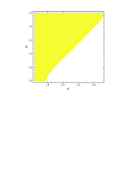
Figure 1: (Color online) The stability domain for fundamental solitons ($S=0$), which is situated on the left-hand side of the plotted curve (the shaded area), in the parameter plane of ($\varepsilon$, $\Omega$), as predicted by the variational approximation, which pertains to the CGL equation with the axisymmetric trapping potential (4). Other parameters are fixed as said above, i.e., $\delta=1/2$, $\mu=1$, and $\nu=-0.1$.

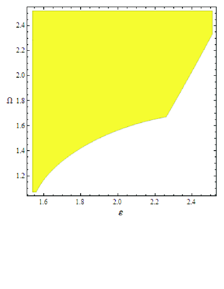
Figure 2: (Color online) The same as in Fig. 1, but for vortex solitons with $S=1$.

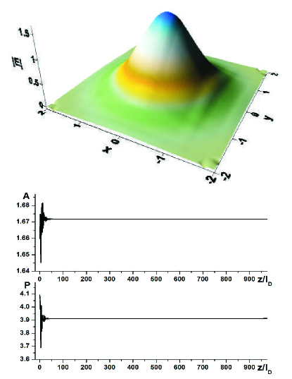
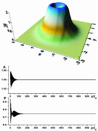
Figure 3: (Color online) Left and right panels display the self-trapping of stable fundamental ($S=0$) and vortical ($S=1$) solitons, respectively, from inputs predicted by the variational approximation, at parameter values $\Omega=1.5$, $\varepsilon=2.2$ for $S=0$, and $\Omega=1.7$, $\varepsilon=2.22$ for $S=1$. The 3D images are the established shapes of the solitons, while plots $A(z/l_{D})$ and $P(z/l_{D})$ show the evolution of the amplitude and total power, see Eq. (6), with $z$ measured in units of the respective diffraction lengths, $l_{D}$.

The VA for dissipative systems, elaborated in Ref. Vladimir , is applied here to look for axisymmetric vortex solutions to Eq. (2) with potential (4), using the following ansatz, written in polar coordinates $r$ and $\theta$:

$$E=A_{0}A\left(\frac{r}{R_{0}R}\right)^{S}\exp\left[R_{0}^{-2}\left(-\frac{r^{2}}{2R^{2}}+iCr^{2}\right)+iS\theta+i\psi\right].$$ (5)

Here, $S$ is the integer vorticity, and real variational parameters are amplitude $A$, width $R$, wave-front curvature (spatial chirp) $C$, and phase $\psi$, that all may be functions of $z$. The ansatz includes normalization factors, $A_{0}=3\cdot 2^{-\left(S+1\right)}\sqrt{\left[3^{3S}\left(2S\right)!\right]/\left[2\left(3S\right)!\right]}$ and $R_{0}=2^{S+1/2}A_{0}^{-1}\sqrt{(S+1)!/\left(2S\right)!}$. A natural characteristic of the soliton is its total power,

$$P=2\pi\int_{0}^{\infty}\left|E(r)\right|^{2}rdr,$$ (6)

which takes value $P=A^{2}R^{2}$ for ansatz (5) (in fact, normalization factors $A_{0}$ and $R_{0}$ were introduced so as to secure this simple expression for $P$).

Skipping technical details, the application of the generalized VA technique, along the lines of Ref. Vladimir , leads to the following system of the first-order evolution equations for the parameters of ansatz (5):

$$\frac{dA}{dz}=\frac{A}{R_{0}^{2}}\left[\frac{3+2S}{2}\varepsilon A^{2}-\frac{5+3S}{4}\mu A^{4}-R_{0}^{2}\delta-2C\right],$$ (7)

$$\frac{dR}{dz}=\frac{R}{2R_{0}^{2}}\left(4C-\varepsilon A^{2}+\mu A^{4}\right),$$ (8)

$$\frac{dC}{dz}=\frac{1}{2R_{0}^{2}}\left(\frac{1}{R^{4}}-\frac{A^{2}}{R^{2}}-\nu\frac{A^{4}}{R^{2}}-4C^{2}-\Omega^{2}R_{0}^{4}\right),$$ (9)

$$\frac{d\psi}{dz}=\frac{(S+1)}{R_{0}^{2}}\left(\frac{3}{2}A^{2}+\frac{5}{4}\nu A^{4}-\frac{1}{R^{2}}\right).$$ (10)

The VA predicts steady states as fixed-point solutions to Eqs. (7)-(9). A straightforward analysis yields two such solutions:

$$A^{2}=\frac{2}{3\mu}\left[\varepsilon\pm\sqrt{\varepsilon^{2}-3\mu R_{0}^{2}\delta\left(S+1\right)^{-1}}\right]\equiv\left(A^{\pm}\right)^{2},$$ (11)

$$R^{2}=2\left[A^{2}(1+\nu A^{2})+\right.$$

$$\left.\sqrt{A^{4}\left[(1+\nu A^{2})^{2}+(\varepsilon-\mu A^{2})^{2}\right]+4\Omega^{2}R_{0}^{4}}\right]^{-1},$$

$$C=\left(A^{2}/4\right)\left(\varepsilon-\mu A^{2}\right).$$

In particular, the nonzero value of $C$ (the wave’s front curvature) in the stationary solution is an essential difference from stationary solitary vortices in conservative models described by the NLS equations.

Further, the calculation of eigenvalues of small perturbations around the fixed points demonstrates that solution $A^{+}$ is stable, while $A^{-}$ is not, cf. Ref. Vladimir . Finally, the VA predicts stability domains for the fundamental ($S=0$) solitons and vortices with $S=1$ in the plane of the free parameters, $\varepsilon$ and $\Omega$. The domains are displayed, respectively, in Figs. 1 and 2, cf. Ref. S.A.D.B.PRB . In these plots, the vertical borders of the stability regions on the left-hand side correspond to the existence condition of solution (11), i.e., $\varepsilon>\sqrt{3\mu R_{0}^{2}\delta\left(S+1\right)^{-1}}$. In particular, for $S=0$ it is $\varepsilon>2\sqrt{2/3}\approx 1.63$, and for $S=1$, the existence region is $\varepsilon>8/\left(3\sqrt{3}\right)\approx 1.54$. These existence limits are found to be in excellent agreement with the corresponding values obtained from direct numerical simulations reported below in Fig. 4.

The accuracy of the solutions for dissipative solitons and vortices predicted by the VA was checked by running direct simulations of the full CGL equation (2), using the respective wave forms, given by Eqs. (5) and (11), as initial conditions. Typical results of such simulations over 1000 diffraction lengths are displayed in Fig. 3, for the solitons with $S=0$ and $S=1$. It is seen that the input wave forms predicted by the VA quickly relax into the finally established soliton shapes, which are shown in Fig. 3.

III Numerical results for vortices in the axisymmetric trapping potential

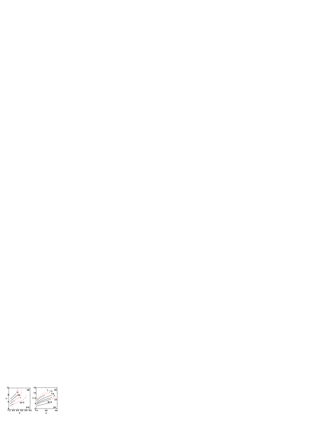
Figure 4: (Color online) The total power, $P$, versus the cubic gain, $\varepsilon$, for families of (a) fundamental solitons ($S=0$) and (b) vortices with $S=1$ at different values of the trapping frequency in potential (4). Solid lines: stable solutions; dotted lines: unstable ones.

Figure 5: (Color online) Examples of stable dissipative solitons with vorticities $S=0$ and $S=1$, for $\varepsilon=1.8$ and potential (4) with $\Omega=2$. Panels (a,c) and (b,d) display the amplitude and phase distributions, respectively.

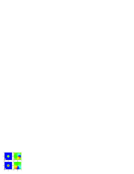
Figure 6: (Color online) The recovery of a perturbed stable vortex soliton with $S=1$ at $\varepsilon=1.8$ and $\Omega=2$, in the case of the axisymmetric potential (4): (a) and (b) initially perturbed amplitude and phase distributions; (c) and (d) self-cleaned amplitude and phase distributions, at $z=200$.

Figure 7: (Color online) The spontaneous breakup of an unstable vortex with $S=1$, which is shown in panels (a) and (b), into a stable dipole soliton, displayed in (c) and (d) at $z=400$. The parameters are $\varepsilon=1.8$ and $\Omega=0.5$, for the axisymmetric potential (4).

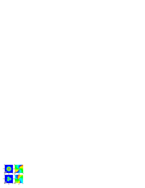
Figure 8: (Color online) The breakup of an unstable vortex with $S=2$, which is shown in panels (a) and (b), into a stable tripole, displayed in (c) and (d) at $z=340$. The parameters are $\varepsilon=1.7$ and $\Omega=0.5$.

Figure 9: (Color online) The generation of a robust rotating tripole in potential (4) from an input cluster formed by three Gaussians with phase differences $2\pi/3$ between them. Left panels: the input field (a), and the established field amplitude $|A(x,y)|$ at $z=300$ (c) and at $z=303$ (e). Right panels: the phase of the input field (b), and the phases of the established pattern at $z=300$ (d) and at $z=303$ (f). The parameters are $\varepsilon=1.7$ and $\Omega=0.5$.

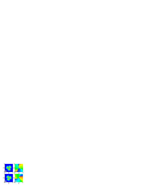
Figure 10: (Color online) The recovery of a perturbed stable tripole, at $\varepsilon=1.7$ and $\Omega=1$, in the axisymmetric trapping potential (4): (a) and (b) perturbed initial distributions of the amplitude and phase; (c) and (d) self-cleaned amplitude and phase distributions at $z=200$.

Figure 11: Power $P$ versus cubic gain $\varepsilon$ for stable dipole solitons (a) and stable tripole solitons (b) trapped in the axisymmetric potential (4), at different values of frequency $\Omega$.

Figure 12: (Color online) The amplitude distribution of the periodic potential, $V(x,y)=p\left[\cos\left(2x\right)+\cos\left(2y\right)\right]$, for $p=1$.

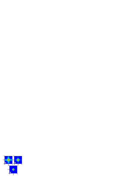
Figure 13: (Color online) The shapes of stable compact (“crater-shaped”) vortices with $S=1$ for $\beta=0$ and $\varepsilon=1.8$. The strength of the periodic potential (3) is $p=1$ (a), $p=2$ (b), and $p=5$ (c).

Figure 14: (Color online) Top: the amplitude (a) and phase (b) of a perturbed compact vortex (“crater”) with $S=1$, for $\beta=0$, $\varepsilon=2$, and $p=2$, in the axisymmetric potential (4). Bottom: the amplitude (c) and phase (d) of the self-cleaned vortex soliton at $z=200$.

Figure 15: Power $P$ versus cubic gain $\varepsilon$ for families of stable compact vortices (“craters”) with $S=1$, at several values of strength $p$ of the periodic potential (3), for $\beta=0$ (a) and $\beta=0.1$ (b).

Figure 16: The same as in Fig. 15, but for families of stable fundamental ($S=0$) solitons.

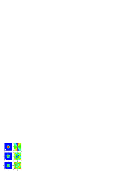
Figure 17: (Color online) A typical example of the generation of a stable quadrupole from an input ring-like field distribution with vorticity $S=2$ (see Eq. 14). Here $p=2$, $\varepsilon=1.8$, and $\beta=0$. (a) input, $z=0$; (b) $z=20$; (c) $z=112$.

Figure 18: Power $P$ versus cubic gain $\varepsilon$ for families of stable quadrupoles at different values of the periodic-potential’s strength, $p$, for $\beta=0$ (a) and $\beta=0.1$ (b).

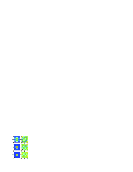
Figure 19: (Color online) The amplitude and phase structure of stable square-shaped quadrupoles for $\beta=0$ and $\varepsilon=2$. The strength of the periodic potential (3) is $p=1$ (a)-(b), $p=2$ (c)-(d), and $p=5$ (e)-(f).

Looking for axisymmetric solutions to Eq. (2) with potential (4) in the numerical form, we substitute $E(z,x,y)=U(z,r)\exp(iS\theta)$, which yields the evolution equation for complex amplitude $U(z,r)$:

$$iU_{z}+\frac{1}{2}\left(U_{rr}+\frac{1}{r}U_{r}-\frac{S^{2}}{r^{2}}U\right)-\frac{1}{2}\Omega^{2}r^{2}U$$

$$+(1-i\varepsilon)|U|^{2}U+(\nu+i\mu)|U|^{4}U+i\delta U=0.$$ (12)

We note that stationary solutions to Eq. (12) must decay exponentially at $r\rightarrow\infty$, and as $r^{|S|}$ at $r\rightarrow 0$.

Stationary dissipative solitons, both fundamental ($S=0$) and vortical ones, were generated as attractors by direct simulations of Eq. (12). To this end, we simulated Eq. (12), starting with the input field in the form of the Gaussian corresponding to vorticity $S$,

$$U_{0}(r)=A_{0}r^{S}\exp\left[-\left(r^{2}/w_{0}^{2}\right)\right],$$ (13)

with real constants $A_{0}$ and $w_{0}$, until the solution would self-trap into a stable dissipative soliton. The so found established solutions can be eventually represented in the form of $U(z,r)=u(r)\exp\left(ikz\right),$ where propagation constant $k$ is, as  a matter of fact, an eigenvalue determined by parameters of Eq. (12).

The simulations of Eq. (12) were run using a 2D Crank-Nicolson finite-difference scheme, with transverse and longitudinal stepsizes $\Delta r=0.05$ and $\Delta z=0.002$. The resulting nonlinear finite-difference equations were solved using the Picard iteration method, and the ensuing linear system was then dealt with using the Gauss-Seidel elimination procedure. To achieve reliable convergence, eight Picard and six Gauss-Seidel iterations were sufficient. The wave number, $k$, was found as the value of the $z$-derivative of the phase of $U(z,r)$. The solution was considered as the established one if $k$ ceased to depend on $z$ and $r$, up to five significant digits. After a particular stationary solution was found by the direct integration of Eq. (12), it was then used as the initial configuration for a new run of simulations, with slightly modified values of the parameters, aiming to generate the solution corresponding to the new values.

When localized states could not self-trap in the course of the evolution, or existed temporarily but eventually turned out to be unstable, $U\left(z,r\right)$ would eventually decay to zero, or evolve into an apparently random pattern filling the entire integration domain. Naturally, the decay to zero was observed when the cubic-gain coefficient, $\varepsilon$, was too small. In the opposite case, with $\varepsilon$ too large, the random pattern was generated.

If the simulations of Eq. (12) converged to stationary localized modes, their full stability was then tested by adding white-noise perturbations at the amplitude level of up to $10\%$, and running direct simulations (in the Cartesian coordinates) of the underlying equation (2). In the course of the stability tests, the evolution of both the total norm, $P(z)$, and the amplitude of the solution was monitored. The solution was identified as a stable one if its amplitude and shape had relaxed back to the unperturbed configuration.

Results of the numerical analysis are summarized in Fig. 4, which represents both stable (solid lines) and unstable (dotted lines) soliton families with $S=0$ and $S=1$, in terms of the dependence of total power $P$ on nonlinear gain $\varepsilon$. The stability of each family is limited to a particular interval, $\varepsilon_{0}<\varepsilon<\varepsilon_{\mathrm{cr}}$ (as said above, at $\varepsilon>\varepsilon_{\mathrm{cr}}$ the solitons evolve into a random pattern filling the entire transverse domain).

Both the VA and direct simulations predict that the stability of the vortices requires relatively large values of trapping frequency $\Omega$. Note that the fundamental solitons ($S=0$) have a stability domain at $\Omega=0$ [see Fig. 4(a)], in accordance with Ref. Lucian . For some values of $\Omega$, the stability intervals predicted by the VA are in good agreement with those produced by the direct simulations: compare, for example, the intervals for the fundamental solitons at $\Omega=1$ in Figs. 1 and 4(a), and for the vortices with $S=1$ at $\Omega=2$ in Figs. 2 and 4(b). However, the agreement is worse in some other cases. Indeed, the VA gives only an approximate prediction for the stability of the zero-vorticity solitons, because ansatz (5) does not accommodate all possible modes of the instability.

Higher-order vortex solitons, with $S\geq 2$, are found to be completely unstable. If vortices with $S=1$ are unstable, they spontaneously split into stable dipoles, whereas those with $S=2$ split into tripoles, see below. Typical examples of the amplitude and phase structure of stable dissipative solitons with vorticities $S=0$ and $S=1$ are displayed in Fig. 5. For the same case, the recovery of the vortex soliton perturbed by the random noise at the $10\%$ amplitude level is displayed in Fig. 6.

IV Dipoles and tripoles in the axisymmetric trap

As said above, the evolution of those vortices with $S=1$ which are unstable, and of the vortices with $S=2$ (recall they all are unstable), leads to their breakup into other types of robust modes, viz., dipoles and tripoles, which feature phase shifts $\pi$ and $2\pi/3$, respectively, between their components. Typical examples of the breakup are displayed in Figs. 7 and 8.

Both the dipole and tripole modes can also be readily generated from initial clusters, formed, respectively, by two Gaussians with the phase shift of $\pi$ between them, or by three Gaussians with phase differences $2\pi/3$. An example of the formation of a stable tripole from the cluster is shown in Fig. 9. Notice the fast rotation of the tripole, which is clearly seen from comparison of panels 9(c) and 9(e). The rotation is possible thanks to the absence of the diffusion, as there is no effective friction that would brake the motion of solitons, cf. Ref. Sakaguchi . Nevertheless, the dipoles generated by the direct numerical simulations do not feature the rotation.

The stability of the dipoles and tripoles was verified by means of systematic direct simulations of initially perturbed patterns, similar to how it was done above for the fundamental solitons and vortices with $S=1$. The random perturbations were imposed at the amplitude level of $10\%$. A typical example of the relaxation of a perturbed stable tripole is displayed in Fig. 10 (the self-cleaning of stable dipoles is quite similar).

Results of the systematic analysis of the stability of the dipole and tripole modes are summarized in terms of the respective $P=P(\varepsilon)$ curves in Fig. 11, cf. Fig. 4 for the fundamental and $S=1$ solitons. The dipole and tripole modes are stable in the intervals of $\varepsilon$ in which curves $P=P(\varepsilon)$ are plotted.

V Stability of crater-shaped vortices and square-shaped quadrupoles in the periodic grating

In this section we consider the model based on the CGL equation (2) with the periodic potential taken as per Eq. (3). Our first objective is to construct the CSVs with $S=1$, which are squeezed, essentially, into a single cell of the grating potential, and identify their stability regions (if any). Note that choosing $p>0$ in Eq. (3) implies the presence of a potential maximum at the center of the grating cell, $x=y=0$. This choice complies with the expected minimum of the local power (the “hole”) at the center of the compact vortex.

Families of relevant solutions were generated by simulating Eq. (2) with potential (3), starting with a Gaussian input corresponding to vorticity $S$, in the form of

$$E_{0}(x,y)=a_{0}\exp\left[-\left(r-r_{0}\right)^{2}/w_{0}^{2}\right]\exp(iS\theta)$$ (14)

[cf. input (13) which created vortices in the axisymmetric parabolic trap (4)], with real constants $a_{0},r_{0}$, and $w_{0}$, in anticipation of a self-trapping of the input field distribution into a ring-shaped pattern with a radius close to $r_{0}$. The so found established dissipative solitons can be eventually represented, as before, in the form of $E(x,y,z)=u(x,y)\exp\left(ikz\right),$ with some propagation constant $k$. This propagation constant was found as the value of the $z$-derivative of the phase of $E(z,x,y)$, at the eventual stage of the evolution, when $k$ ceased to depend on $x$, $y$ and $z$, up to five significant digits. The stability of the solitons was then tested, as before, against random perturbations with the relative amplitude of up to $10\%$.

As in the previous section, the Crank-Nicolson algorithm was used for the numerical simulations, with transverse and longitudinal stepsizes $\Delta x=\Delta y=0.1$ and $\Delta z=0.005$, for the grating strength $p=1$. For larger values of $p$, it was necessary to use smaller stepsizes: $\Delta x=\Delta y=0.08$, $\Delta z=0.004$ for $p=2$, and $\Delta x=\Delta y=0.06$, $\Delta z=0.003$ for $p=5$. Using the same algorithm as mentioned above, the nonlinear finite-difference equations were solved using the Picard iteration method, and the resulting linear system was handled by means of the Gauss-Seidel iterative procedure. To achieve good convergence, ten Picard and five Gauss-Seidel iterations were needed.

In Fig. 12 we show an illustrative plot of the 2D periodic potential (3) with strength $p=1$. The numerical simulations demonstrate that fully stable CSVs may be indeed supported by the periodic potential (3), see Figs. 13 and 14. This result is significant, as no example of stable compact vortices, squeezed into a single cell of the supporting lattice, was earlier reported in 2D CGL models. A set of typical examples of stable craters is displayed in Fig. 13, and the stability of such vortices (in the form of the self-cleaning against random perturbations) is illustrated by Fig. 14. Further analysis (not shown here) demonstrate that the shape of the craters and their self-cleaning after the addition of random perturbations seem essentially the same if the diffusion term with a small coefficient $\beta$ is added (which means that the grating’s potential remains a stronger stabilizing factor than the weak diffusion, if any).

In Fig. 15, the CSV families with $S=1$ are represented, as before, by the corresponding $P(\varepsilon)$ curves, which are plotted in intervals of values of the cubic gain $\varepsilon$ where the CSVs are stable. For the sake of comparison, in Fig. 16 we display similar diagrams for the fundamental solitons ($S=0$) in the same model. In Figs. 15 and 16, we additionally display the stability domains found at a small nonzero value of the diffusion parameter, $\beta=0.1$. The comparison demonstrates that the stability regions for both the fundamental solitons and compact vortices shift to larger values of $\varepsilon$ at $\beta>0$, which is natural, as a larger value of the cubic gain is needed to compensate the loss incurred by the diffusion term.

Stable CSVs with vorticities $S=2$ have not been found in direct simulations of Eq. (2) with the periodic potential; instead, families of robust compact square-shaped quadrupoles, into which unstable vortices with $S=2$ are spontaneously transformed, were found at different values of the periodic-potential’s strength, $p$. A typical example of the transformation, for $a_{0}=1.2$, $r_{0}=0.7$, and $w_{0}=1$, is displayed in Fig. 17. The stability of the quadrupoles against random perturbations was tested in the same way as done above for the vortices with $S=1$. The results are again summarized by means of the respective $P(\varepsilon)$ curves, which are displayed, both for $\beta=0$ and $\beta=0.1$, in Fig. 18. Finally, in Fig. 19 we show typical examples of the amplitude and phase structure of compact square-shaped quadrupoles for $\beta=0$, $\varepsilon=2$, and three different values of the strength of the periodic potential, $p=1,2$, and $5$.

VI Conclusions

The major objective of this work was to build stable compact crater-shaped vortices, with topological charge $S=1$, in the complex Ginzburg-Landau model which is relevant to modeling laser cavities, as it does not include the artificial diffusion term. Instead, the stabilization of the compact vortices is provided by external potentials, which we took in two different forms: as the axisymmetric parabolic trap (4), and the periodic grating’s potential (3). In the experiment, the effective axisymmetric potential can be realized by means of a simple focusing lens inserted into the cavity. In both cases, stability regions for the crater-shaped vortices have been identified. Parallel to that, the stability regions of the fundamental solitons ($S=0$) were also found, for the sake of the comparison. In the case of the axisymmetric potential, those crater-shaped vortices which are unstable split into robust dipoles. All the vortices with $S=2$ are unstable, splitting into stable tripoles, that may freely rotate. The stability regions for the dipole and tripole modes were identified too. As concerns the periodic potential, it cannot stabilize crater-shaped vortices with $S>1$. Instead, families of stable compact square-shaped quadrupoles were found to exist at different values of the strength of the periodic potential.

A challenging extension suggested by the present work is to find stable compact solitons with embedded vorticity in the three-dimensional (spatiotemporal) version of the complex Ginzburg-Landau equation with the periodic potential. This possibility is especially interesting because this model does not support stable compound vortices latest .

References

- (1) I. S. Aranson and L. Kramer, Rev. Mod. Phys. 74, 99 (2002); B. A. Malomed, in Encyclopedia of Nonlinear Science, p. 157, A. Scott (Ed.), Routledge, New York, 2005.
- (2) N. Akhmediev and A. Ankiewicz (Eds.), Dissipative Solitons: From Optics to Biology and Medicine, Lect. Notes Phys. 751 (Springer, Berlin, 2008).
- (3) N. N. Rosanov, Spatial Hysteresis and Optical Patterns (Springer, Berlin, 2002); S. Barland et al., Nature (London) 419, 699 (2002); Z. Bakonyi, D. Michaelis, U. Peschel, G. Onishchukov, and F. Lederer, J. Opt. Soc. Am. B 19, 487 (2002); E. A. Ultanir, G. I. Stegeman, D. Michaelis, C. H. Lange, and F. Lederer, Phys. Rev. Lett. 90, 253903 (2003); P. Mandel and M. Tlidi, J. Opt. B: Quantum Semiclass. Opt. 6, R60 (2004); N. N. Rosanov, S. V. Fedorov, and A. N. Shatsev, Appl. Phys. B 81, 937 (2005); C. O. Weiss and Ye. Larionova, Rep. Progr. Phys. 70, 255 (2007); N. Veretenov and M. Tlidi, Phys. Rev. A 80, 023822 (2009); P. Genevet, S. Barland, M. Giudici, and J. R. Tredicce, Phys. Rev. Lett. 104, 223902 (2010).
- (4) B. A. Malomed, Physica D 29, 155 (1987); O. Thual and S. Fauve, J. Phys. (Paris) 49, 1829 (1988); S. Fauve and O. Thual, Phys. Rev. Lett. 64, 282 (1990); W. van Saarloos and P. C. Hohenberg, Phys. Rev. Lett. 64, 749 (1990); V. Hakim, P. Jakobsen, and Y. Pomeau, Europhys. Lett. 11, 19 (1990); B. A. Malomed and A. A. Nepomnyashchy, Phys. Rev. A 42, 6009 (1990); P. Marcq, H. Chaté, R. Conte, Physica D 73, 305 (1994); N. Akhmediev and V. V. Afanasjev, Phys. Rev. Lett. 75, 2320 (1995); H. R. Brand and R. J. Deissler, Phys. Rev. Lett. 63, 2801 (1989); R. J. Deissler and H. R. Brand, ibid. 72, 478 (1994); V. V. Afanasjev, N. Akhmediev, and J. M. Soto-Crespo, Phys. Rev. E 53, 1931 (1996); J. M. Soto-Crespo, N. Akhmediev, and A. Ankiewicz, Phys. Rev. Lett. 85, 2937 (2000); H. Leblond, A. Komarov, M. Salhi, A. Haboucha, and F. Sanchez, J. Opt. A: Pure Appl. Opt. 8, 319 (2006); W. H. Renninger, A. Chong, and F. W. Wise, Phys. Rev. A 77, 023814 (2008); J. M. Soto-Crespo, N. Akhmediev, C. Mejia-Cortes, and N. Devine, Opt. Express 17, 4236 (2009); D. Mihalache and D. Mazilu, Rom. Rep. Phys. 61, 175 (2009); D. Mihalache, J. Optoelectron. Adv. Mat. 12, 12 (2010); Y. J. He, B. A. Malomed, D. Mihalache, F. W. Ye, and B. B. Hu, J. Opt. Soc. Am. B 27, 1266 (2010).
- (5) B. A. Malomed, D. Mihalache, F. Wise, and L. Torner, J. Opt. B: Quantum Semiclass. Opt. 7, R53 (2005).
- (6) A. S. Desyatnikov, Y. S. Kivshar, and L. Torner, Progr. Opt. 47, 291 (2005).
- (7) W. J. Firth and D. V. Skryabin, Phys. Rev. Lett. 79, 2450 (1997); L. Torner and D. V. Petrov, Electron. Lett. 33, 608 (1997); D. V. Petrov, L. Torner, J. Martorell, R. Vilaseca, J. P. Torres, and C. Cojocaru, Opt. Lett. 23, 1787 (1998).
- (8) V. I. Petviashvili and A. M. Sergeev, Dokl. AN SSSR 276, 1380 (1984) [Sov. Phys. Doklady 29, 493 (1984)].
- (9) L.-C. Crasovan, B. A. Malomed, and D. Mihalache, Phys. Rev. E 63, 016605 (2001); Phys. Lett. A 289, 59 (2001).
- (10) D. Mihalache, D. Mazilu, F. Lederer, Y. V. Kartashov, L.-C. Crasovan, L. Torner, and B. A. Malomed, Phys. Rev. Lett. 97, 073904 (2006); D. Mihalache, D. Mazilu, F. Lederer, H. Leblond, and B. A. Malomed, Phys. Rev. A 76, 045803 (2007); ibid. 75, 033811 (2007).
- (11) J. Lega, J. V. Moloney, and A. C. Newell, Phys. Rev. Lett. 73, 2978 (1994); Physica D 83, 478 (1995).
- (12) H. Leblond, B. A. Malomed, and D. Mihalache, Phys. Rev. A 80, 033835 (2009).
- (13) A. Szameit, J. Burghoff, T. Pertsch, S. Nolte, and A. Tünnermann, Opt. Exp. 14, 6055 (2006).
- (14) J. W. Fleischer, M. Segev, N. K. Efremidis, and D. N. Christodoulides, Nature 422, 147 (2003).
- (15) H. Leblond, M. Salhi, A. Hideur, T. Chartier, M. Brunel, and F. Sanchez, Phys. Rev. A 65, 063811 (2002); A. Komarov, H. Leblond, and F. Sanchez, Phys. Rev. E 72, 025604(R) (2005); M. Salhi, A. Haboucha, H. Leblond, F. Sanchez, Phys. Rev. A 77, 033828 (2008).
- (16) B. B. Baizakov, B. A. Malomed, and M. Salerno, Europhys. Lett. 63, 642 (2003); T. Mayteevarunyoo, B. A. Malomed, B. B. Baizakov, and M. Salerno, Physica D 238, 1439 (2009).
- (17) J. Yang and Z. H. Musslimani, Opt. Lett. 28, 2094 (2003); J. Wang and J. Yang, Phys. Rev. A 77, 033834 (2008).
- (18) D. N. Neshev, T. J. Alexander, E. A. Ostrovskaya, Y. S. Kivshar, H. Martin, I. Makasyuk, and Z. Chen, Phys. Rev. Lett. 92, 123903 (2004); J. W. Fleischer, G. Bartal, O. Cohen, O. Manela, M. Segev, J. Hudock, and D. N. Christodoulides, ibid. 92, 123904 (2004).
- (19) R. Driben, B. A. Malomed, A. Gubeskys, and J. Zyss, Phys. Rev. E 76, 066604 (2007).
- (20) R. Driben and B. A. Malomed, Eur. Phys. J. D 50, 317 (2008).
- (21) A. Gubeskys and B. A. Malomed, Phys. Rev. A 76, 043623 (2007).
- (22) H. Sakaguchi and B. A. Malomed, Europhys. Lett. 72, 698 (2005).
- (23) H. Sakaguchi and B. A. Malomed, Phys. Rev. A 79, 043606 (2009).
- (24) T. J. Alexander and L. Bergé, Phys. Rev. E 65, 026611 (2002); D. Mihalache, D. Mazilu, B. A. Malomed, and F. Lederer, Phys. Rev. A 73, 043615 (2006); L. D. Carr and C. W. Clark, Phys. Rev. Lett. 97, 010403 (2006).
- (25) V. Skarka and N. B. Aleksić, Phys. Rev. Lett. 96, 013903 (2006); N. B. Aleksić, V. Skarka, D. V. Timotijević, and D. Gauthier, Phys. Rev. A 75, 061802 (2007); V. Skarka, D. V. Timotijević, and N. B. Aleksić, J. Opt. A: Pure Appl. Opt. 10, 075102 (2008).
- (26) B. A. Malomed, in: Progr. Optics 43, 71 (E. Wolf, editor: North Holland, Amsterdam, 2002).
- (27) V. Skarka, N. B. Aleksić, M. Derbazi, and V. I. Berezhiani, Phys. Rev. B 81, 035202 (2010).
- (28) H. Sakaguchi, Physica D 210, 138 (2005); G. Wainblat and B. A. Malomed, ibid. 238, 1143 (2009).
- (29) D. Mihalache, D. Mazilu, F. Lederer, H. Leblond, and B. A. Malomed, Phys. Rev. A 81, 025801 (2010).