Non-equilibrium frequency-dependent noise through a quantum dot: A real time functional renormalization group approach

Abstract

We construct a real time current-conserving functional renormalization group (RG) scheme on the Keldysh contour to study frequency-dependent transport and noise through a quantum dot in the local moment regime. We find that the current vertex develops a non-trivial non-local structure in time, governed by a new set of RG equations. Solving these RG equations, we compute the complete frequency and temperature-dependence of the noise spectrum. For voltages large compared to the Kondo temperature, $eV\gg k_{B}T_{K}$, two sharp anti-resonances are found in the noise spectrum at frequencies $\hbar\omega=\pm eV$, and correspondingly, two peaks in the ac conductance through the dot.

Introduction. Not only the current flowing through a system, but also its fluctuations (noise) carry crucial information on the physics that governs transport landauer . Zero-frequency noise (shot noise) has been used, e.g., to reveal the fractional charge of the quasiparticle excitations in the fractional quantum Hall liquid glattli . The low-frequency electrical noise has been extensively studied in various systemsblanter and is by now relatively well understood. However, even more information is stored in the finite-frequency (FF) current noise: It has been predicted that the FF noise is sensitive to the statistics of the quasiparticles statistics and a crossover between different quantum statistics can be potentially observed as function of frequency, similar to the one observed as a function of temperature Heiblum . Moreover, in the quantum regime characterized by frequencies higher than the applied voltage or temperature, the FF noise is a powerful tool to reveal the characteristic time scales of the probed system gabelli as well as the dynamics of the excitations or the importance of interactions.

Due to their small size, transport through quantum dots (QD) is strongly influenced by the Coulomb blockade. In particular, QDs with an odd number of electrons behave as artificial magnetic impurities and exhibit the Kondo effect david , a paradigmatic many-body phenomenon corresponding to the screening of the spin of the quantum dot by the conduction electrons of the leads at temperatures $T$ below the Kondo temperature, $T_{K}$. QDs thus provide an ideal test ground to study non-equilibrium transport in the presence of strong interactions. While the conductance of a QD in the Kondo regime is well understood by now glazman-review , much less is known about current-fluctuations. Though these are promising quantities to characterize the out of equilibrium Kondo effect, nevertheless, most experiments focused so far on measurements of the average current franceschi02 ; paaske06 ; grobis08 , and even results on low-frequency noise measurements have only appeared recently delattre09 . While the effect of ac voltage on the non-equilibrium Kondo effect has been studied experimentally relatively longtime ago kogan04 , no FF noise measurements have been reported so far to our knowledge. Theoretically, most studies focused on shot noise: a non-monotonous bias-dependence of the shot noise with a maximum at $eV\sim k_{B}T_{K}$ has been found at $T\ll T_{K}$ meir02 , and a universal ratio $5/3e$ between the shot noise and the backscattering current at $T=0$ has been predicted for the $SU(2)$ Kondo effect sela06 .

The purpose of this work is to provide a general analysis of the finite-frequency current noise through a quantum dot in the local moment regime. To achieve this, we construct a real time functional renormalization group (FRG) scheme on the Keldysh contour to study frequency-dependent transport and noise through a Kondo quantum dot. Our formalism reproduces the scaling equations of Rosch et al. rosch for the vertex function. However, we find that the current vertex also develops a non-trivial non-local structure in time, governed by a new set of RG equations. Such structure of the current vertex turns out to be unavoidable to guarantee current conservations and is necessary to calculate the finite frequency current noise in a controlled manner. Solving this set of RG equations, we compute the complete frequency and temperature dependent noise spectrum through the dot. Our approach is valid at any frequency $\omega$, voltage $V$ and temperature $T$ provided that ${\rm max}\{eV,k_{B}T\}>k_{B}T_{K}$. For frequencies $\hbar\omega\gg k_{B}T_{K}$, we find sharp anti-resonances in the voltage dependence of the noise spectrum at $eV=\hbar\omega$, which gradually disappear with increasing temperature. The absorption noise is also found to exhibit strong anomalies at $\hbar\omega=eV$, and we find similar anomalies in the non-equilibrium ac conductance, too, where a split non-equilibrium Kondo resonance is observed. Precursors of the noise anomaly have been found in the zero-temperature symmetrized noise at finite frequency, as first computed at the Toulouse point of the Kondo model schiller , and later confirmed by a non-equilibrium one-loop perturbative calculation schoeller . However, logarithmic singularities are completely absent at the rather special Toulouse point schiller , while the method of Ref. schoeller was not accurate enough to capture fine details of the anomaly.

Model. In this paper, we focus our attention to the local moment regime of the quantum dot, where we can describe the electron on the dot as a spin $S=1/2$ moment which couples to electrons in the left and right electrodes through an exchange interaction glazman-review ,

$$H_{\rm int}=\frac{1}{2}\sum_{\alpha,\beta=L,R}\sum_{\sigma,\sigma^{\prime}}j_{\alpha\beta}\;\mathbf{S}\;\psi_{\alpha\sigma}^{\dagger}{\mathbf{\mathbf{\sigma}}}_{\sigma\sigma^{\prime}}\psi_{\beta\sigma^{\prime}}\;.$$ (1)

Here $\mathbf{\sigma}$ stands for the three Pauli matrices, the fields $\psi_{\alpha\sigma}=\int c_{\alpha\sigma}(\xi)e^{-|\xi|a}\;d\xi$ destroy electrons of spin $\sigma$ in leads $\alpha\in\{L,R\}$, with $1/a$ a high energy cut-off  . The dynamics of $\psi_{\alpha\sigma}$ is governed by the non-interacting Hamiltonian, $H_{0}=\sum_{\alpha,\sigma}\int{\rm d}\xi\;(\xi+\mu_{\alpha})\;c^{\dagger}_{\alpha\sigma}(\xi)c_{\alpha\sigma}(\xi)$, with $\mu_{\alpha}=eV_{\alpha}$, the chemical potential shift of lead $\alpha$.

To describe the spin using standard field-theoretical methods, we make use of Abrikosov’s pseudo-fermion representation Abrikosov : we introduce a fermion operator $f^{\dagger}_{s}$ for each spin component, $s=\pm 1/2$, and represent the spin operator as $\hat{S}^{i}\to\sum_{s,s^{\prime}}\frac{1}{2}\;f^{\dagger}_{s}\sigma^{i}_{s,s^{\prime}}f_{s^{\prime}}$ with the additional constraint, $\sum_{s}f^{\dagger}_{s}f_{s}=1$.

We then employ a path integral formalism on the Keldysh contour. In this approach each fermionic field is replaced by two time-dependent Grassmann fields living on the upper and lower Keldysh contour ($\kappa=1,2$), respectively, and the dynamics is determined by the Keldysh action, ${\cal S}={\cal S}_{\rm lead}+{\cal S}_{\rm spin}+{\cal S}_{\rm int}$. The parts ${\cal S}_{\rm lead}$ and ${\cal S}_{\rm spin}$ describe the conduction electrons and the spin in the absence of interaction. They are quadratic in the fields, and determine the non-interacting Green’s functions epaps .

The interaction part of the action, ${\cal S}_{\rm int}$, is diagonal in the Keldysh indices and is initially local in time. However, elimination of high energy degrees of freedom in course of the RG procedure generates retardation effects, and the interaction becomes non-local. We find that, with a good approximation, it can be expressed as

$${\cal S}_{\rm int} = \sum_{\kappa}\sum_{\alpha,\beta}s_{\kappa}\;\frac{1}{4}\int{\rm d}t_{1}\;{\rm d}t_{2}\;g_{\alpha\beta}(t_{1}-t_{2})\;$$ (2)

$$\bar{f}^{\kappa}(T_{12})\vec{\sigma}f^{\kappa}(T_{12})\cdot\bar{\psi}^{\kappa}_{\alpha}(t_{1})\vec{\sigma}\psi_{\beta}^{\kappa}(t_{2})\;,$$

where $T_{12}=(t_{1}+t_{2})/2$ and $s_{\kappa}=\pm 1$ for the upper and lower Keldysh contours, respectively. The initial (bare) coupling function $g_{\alpha\beta}(t)$ is local in time, and is given by $g^{(0)}_{\alpha\beta}(t)=j_{\alpha\beta}\;\delta(t)$. The justification for this structure, Eq. (2), is straightforward: The spin evolves very slowly, and its time evolution can be very well approximated by the one in the absence of interactions at electronic time scales. However, conduction electrons have fast dynamics, and their retardation effects become important as one approaches smaller energy scales.

Functional RG. We construct the RG equations by expanding the action in ${\cal S}_{\rm int}$ and rescaling the cutoff parameter $a\to a^{\prime}$. An integro-differential equation is obtained for the functions $g_{\alpha\beta}(t)$, which becomes simple in Fourier space,

$$\frac{{\rm d}{\bf g}(\omega)}{{\rm d}l}={\bf g}(\omega)\;{\bf q}(\omega,a)\;{\bf g}(\omega)\;.$$ (3)

Here $l=\ln(a/a_{0})$ is the scaling variable, $a_{0}$ is the initial value of the cut-off time, and we introduced the matrix notation, $g_{\alpha\beta}\to{\bf g}$. The matrix ${\bf q}(\omega,a)$ is a cut-off function, which depends somewhat on the precise cut-off scheme, but for practical purposes is well-approximated by the function $q_{\alpha\beta}(\omega,a)\approx\delta_{\alpha\beta}\;\Theta(\frac{1}{a}-|\omega-\mu_{\alpha}|)$ at $T=0$ temperature rosch . The scaling equation, Eq. (3), is identical to the one obtained in a more heuristic way in Ref. rosch , however, in our real time functional RG formalism the derivation is rather straightforward and simple long . We remark that the usual poor man’s RG procedure can be recovered by dropping the time-dependence of $g_{\alpha\beta}$, and replacing the generated non-local couplings by local ones, $g_{\alpha\beta}(t)\to\delta(t)\;\int{\rm d}t\;g_{\alpha\beta}(t)$, which corresponds to setting $\omega\to 0$ in Eq. (3).

Our primary purpose is to compute current-current correlation functions. To do that, we first define the left and right current operators from the equation of motion, giving $\hat{I}_{L}(t)=-\hat{I}_{R}(t)=\sum_{\alpha\beta}\frac{e}{2}v^{L}_{\alpha\beta}\hat{\bf S}(t)\cdot\hat{\psi}^{\dagger}_{\alpha}(t)\mathbf{\sigma}\hat{\psi}_{\beta}(t)$, with the current vertex matrices defined as

$${\bf v}^{L}=-{\bf v}^{R}=\begin{pmatrix}0&-i\;j_{LR}\\ i\;j_{LR}&0\end{pmatrix}\;.$$ (4)

In the path integral language, it is useful to introduce a corresponding generating functional,

$$Z[h_{\alpha}^{\kappa}(t)]\equiv\langle e^{-i\;\sum_{\kappa,\alpha}\int{\rm d}t\;h_{\alpha}^{\kappa}(t)I^{\kappa}_{\alpha}(t)}\rangle_{\cal S}\;,$$ (5)

from which the current-current correlation functions can be generated by functional differentiation with respect to $h_{\alpha}^{\kappa}(t)$. A systematic investigation of the leading logarithmic diagram series shows that the expression of the current field, $I^{\kappa}(t)$, necessarily becomes non-local in time under the RG procedure, and acquires a form,

$$I^{\kappa}_{L}(t) = \frac{e}{4}\sum_{\kappa}\sum_{\alpha\beta}\int{\rm d}t_{1}{\rm d}t_{2}\;V_{\alpha\beta}^{L}(t_{1}-t,t-t_{2},a)\;$$ (6)

$$\bar{f}^{\kappa}(t)\vec{\sigma}f^{\kappa}(t)\cdot\bar{\psi}^{\kappa}_{\alpha}(t_{1})\vec{\sigma}\psi^{\kappa}_{\beta}(t_{2})\;.$$

The physical motivation of the double time-structure is simple: in the renormalized theory it is not enough to know the times electrons enter and leave the dot ($t_{1,2}$), but the time of the current measurement, $t$, must also be kept track of.

It is relatively straightforward to derive the scaling equations from the perturbative expansion of Eq. (5), and we obtain

$$\frac{{\rm d}{\bf V}^{L}(\omega_{1},\omega_{2})}{{\rm d}l} = {{\bf V}^{L}(\omega_{1},\omega_{2})}\;{\bf q}(\omega_{2},a)\;{\bf g}(\omega_{2})\;$$ (7)

$$+ {\bf g}(\omega_{1})\;{\bf q}(\omega_{1},a)\;{{\bf V}^{L}(\omega_{1},\omega_{2})}\;.$$

This equation needs be solved parallel to the scaling equation, Eq. (3) with the boundary condition, ${\bf V}^{L/R}(\tau_{1},\tau_{2},a_{0})=\delta(\tau_{1})\;\delta(\tau_{2})\;{\bf v}^{L/R}$. Though the renormalized couplings ${\bf g}_{L}(\omega)$ drive the scaling of the current vertexes, ${\bf V}_{L}(\omega_{1},\omega_{2},a_{0})$, there seems to be no simple connection between these too. In other words, it is unavoidable to introduce the renormalized current vertexes within the functional RG scheme to compute time-dependent current correlations. The above extension seems to be also necessary to guarantee current conservation: Eq. (7) is linear in ${\bf V}^{L}$, and therefore the condition $I^{\kappa}_{L}(t)+I^{\kappa}_{R}(t)\equiv 0$ is automatically satisfied, for any value of the cut-off, $a$. On the other hand, we could not find any way to generate a current field from just the renormalized action, Eq. (2), such that it respects current conservation.

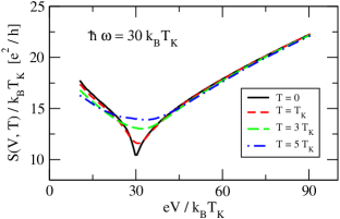
Figure 1: (color online) Voltage-dependence of the symmetrical noise, as computed by FRG for $\hbar\omega=30\;k_{B}T_{K}$.

We solved Eqs. (3) and (7) numerically to obtain ${\bf g}$ and ${\bf V}^{L/R}$. Both display singularities at frequencies $\hbar\omega=\pm eV/2$ epaps . With the couplings ${\bf g}(\omega_{1})$ and the current vertexes ${\bf V}^{L/R}(\omega_{1},\omega_{2})$ in hand, we then proceeded to compute the noise through the device, by doing perturbation theory with the renormalized action. For the Fourier transform of the absorption and emission noise components $S_{LL}^{>}(t)\equiv\langle\hat{I}_{L}(t)\hat{I}_{L}(0)\rangle$, and $S_{LL}^{<}(t)\equiv\langle\hat{I}_{L}(0)\hat{I}_{L}(t)\rangle$, we obtain $S_{LL}^{>}(\omega)=S_{LL}^{<}(-\omega)$, with

$$S_{LL}^{>}(\omega) = \frac{e^{2}}{2}\;S(S+1)\int\frac{{\rm d}\tilde{\omega}}{2\pi}\;{\rm Tr}\{{\bf V}^{L}(\tilde{\omega}_{-},\tilde{\omega}_{+})$$ (8)

$${\bf G}^{>}(\tilde{\omega}_{+}){\bf V}^{L}(\tilde{\omega}_{+},\tilde{\omega}_{-}){\bf G}^{<}(\tilde{\omega}_{-})\}\;.$$

Here $\tilde{\omega}_{\pm}=\tilde{\omega}\pm\frac{\omega}{2}$, and the bigger and lesser Green’s functions $G_{\alpha\beta}^{>/<}(\omega)=\pm i\;2\pi\;\delta_{\alpha\beta}\;f(\pm(\omega-\mu_{\alpha}))$.

Results. The symmetrized noise spectrum, $S_{LL}(\omega)\equiv\frac{1}{2}[S^{>}_{LL}(\omega)+S^{<}_{LL}(\omega)]$ is plotted in Fig. 1 for $\hbar\omega=30\;k_{B}T_{K}$ as a function of voltage, $V$. Clearly, the noise spectrum shows rather strong features at the bias voltages, $eV\approx\hbar\omega$. The appearing dips are clear fingerprints of the non-equilibrium Kondo effect, and they gradually vanish as we increase the temperature, $T$ . The increase in the noise with decreasing $V$ at low voltages can be understood as being the consequence of increasing spin relaxation time, resulting in an increased Kondo conductance through the dot. At high voltages, on the other hand, increased photon emission is mainly responsible for the increasing noise, thereby giving the V-shaped pattern.

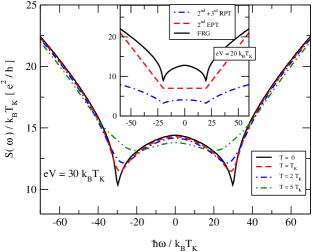
Figure 2: (color online) Temperature-dependence of the symmetrical noise, as computed by FRG. Inset: Comparison with third order renormalized perturbation theory (RPT) using a reduced cut-off, $\tilde{a}=\hbar/10eV$ and the corresponding couplings $j_{LR}(\tilde{a})$, and effective second order perturbation theory with renormalized couplings $j_{LR}(\tilde{a}=\hbar/eV)$, but still using the original bandwidth. None of these methods are able to get close to the FRG results.

Similar features appear in the frequency-dependent symmetrized noise (see Fig. 2). It is instructive to compare the FRG results with perturbation theory, giving

$$S^{>}_{LL}(t) = -e^{2}\;\frac{3}{4}|j_{LR}|^{2}\cos(eVt)\Bigl{\{}\frac{1}{(t-i\;a)^{2}}$$ (9)

$$+ 2(j_{LL}+j_{RR})\frac{\ln(1+i\;t/a)}{t(t-2\;i\;a)}+\dots\Bigr{\}}\;.$$

The curves in the inset of Fig. 2 are obtained by taking the Fourier transform of this expression. While the perturbative result also exhibits singular features at $\hbar\omega=\pm eV$, however, it does not reproduce the precise shape of the anomaly, even if we use renormalized parameters, $j_{\alpha\beta}\to j_{\alpha\beta}(eV)$ obtained by solving the usual leading logarithmic scaling equations.

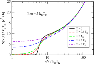
Figure 3: (color online) Voltage and temperature-dependence of the emission noise as computed through FRG for $\hbar\omega=5k_{B}T_{K}$.

Experimentally, it may be more convenient to measure separately the emission or absorption noise components at a fixed finite frequency, $S_{e/a}(\omega>0)\equiv S^{<}(\pm\omega)$, as function of the bias voltage basset . As shown in Fig. 3, at $T=0$ the emission noise vanishes at voltages $V<\hbar\omega/e$ due to energy conservation, and has an abrupt logarithmic singularity at $V=\hbar\omega/e$ at temperatures $T\ll T_{K}$, which is gradually smeared out for $k_{B}T>eV$.

Another quantity which may be easier to access experimentally is the non-equilibrium finite frequency linear conductance, defined as the current response of the system to an external time-dependent variation of one of the lead potentials. According to a formula of Safi safi , this can be expressed as

$${\rm Re}\,G_{LL}(\omega,V)=\frac{1}{\hbar\omega}(S_{LL}^{>}(\omega)-S_{LL}^{<}(\omega))\;.$$ (10)

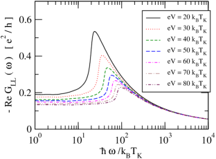
Figure 4: (color online) The ac conductance for $\omega>0$.

Notice that $G_{LL}(0,V)$ is just the usual non-equilibrium differential conductance, $G_{LL}(0,V)=\partial_{V_{L}}\langle\hat{I}_{L}\rangle$, while $G_{LL}(\omega,V\to 0)$ corresponds to the usual equilibrium ac conductance sindel . ${\rm Re}\,G_{LL}(\omega,V)$ is an even function of $\omega$ and exhibits two peaks at $\hbar\omega=\pm eV$, associated with the non-equilibrium Kondo effect meir02 (see Fig. 4) . This confirms that the dips in the noise are related to the splitting of the Kondo resonance at a finite bias.

Summary. We have developed a real-time functional renormalization group approach. We have shown that the current vertex becomes non-local in time under renormalization which turns out to be necessary in order to ensure non-equilibrium current conservation. Within this formalism, we have been able to calculate the voltage and temperature dependence of the current noise at finite frequency and the non-equilibrium ac conductance, quantities which are within experimental reach basset .

Acknowledgment. We would like to thank J. Basset, R. Deblock, H. Bouchiat, and B. Reulet for interesting discussions. This research has been supported by Hungarian grants OTKA Nos. NF061726, K73361, Romanian grant CNCSIS PN II ID-672/2008, the EU GEOMDISS project, and Taiwan’s NSC grant No.98-2918-I-009-06, No.98-2112-M-009-010-MY3, the MOE-ATU program and the NCTS of Taiwan, R.O.C.. C.H.C. acknowledges the hospitality of Yale University.

References

- (1) R. Landauer, Nature 392, 658 (1998).
- (2) L. Saminadayar et al., Phys. Rev. Lett. 79, 2526 (1997); R. de-Piciotto et al., Nature (London) 389, 162 (1997).
- (3) Ya. M. Blanter and M. B\a”uttiker, Phys. Rep. 336, 1 (2000).
- (4) I. Safi, P. Devillars, and T. Martin, Phys. Rev. Lett. 86, 4628 (2001); S. Vishveshwara, ibid 91, 196803 (2003); C. Bena and C. Nayak, Phys. Rev. B 73, 155335 (2006).
- (5) A. Bid, et al., Phy. Rev. Lett. 103, 236802 (2009).
- (6) J. Gabelli and B. Reulet, Phys. Rev. Lett. 100, 026601 (2008).
- (7) D. Goldhaber-Gordon et al., Nature 391, 156 (1998); S. M. Cronenwett et al., Science 281 540 (1998).
- (8) L.I. Glazman, M. Pustilnik, Lectures notes of the Les Houches Summer School 2004 in ”Nanophysics: Coherence and Transport,” eds. H. Bouchiat et al. (Elsevier, 2005), pp. 427-478.
- (9) S. De Franceschi et al., Phys. Rev. Lett 89, 156801 (2002).
- (10) J. Paaske et al., Nature Phys. 2, 460 (2006).
- (11) M. Grobis et al., Phys. Rev. Lett. 100, 246601 (2008).
- (12) T. Delattre et al., Nature Phys. 5, 208 (2009).
- (13) A. Kogan, S. Amasha, M.A. Kastner, Science 304, 1293 (2004).
- (14) Y. Meir and A. Golub, Phys. Rev. Lett. 88, 116802 (2002).
- (15) E. Sela, Y. Oreg, F. von Oppen, an J. Koch, Phys. Rev. Lett. 97, 086601 (2006); A. O. Gogolin and A. Komnik, Phys. Rev. Lett. 97, 016602 (2006).
- (16) A. Rosch, J. Kroha, and P. W\a”olfle, Phys. Rev. Lett. 87, 156802 (2001); A. Rosch, J. Paaske, J. Kroha, and P. W\a”olfle, ibid 90, 076804 (2003).
- (17) A. Schiller and S. Hershfield, Phys. Rev. B 58, 14978 (1998).
- (18) T. Korb, F. Reininghaus, H. Schoeller, and J. K\a”onig, Phys. Rev. B 76, 165316 (2007).
- (19) A. A. Abrikosov, Physics 2, 5 (1965).
- (20) See supplementary EPAPS document.
- (21) C.P. Moca et al., in preparation.
- (22) J. Basset, H. Bouchiat, and R. Deblock, . arXiv:1006.0892.
- (23) I. Safi, arXiv:0908.4382 (see also I. Safi, C. Bena, and A. Cr\a’epieux, Phys. Rev. B 78 205422 (2008) ).
- (24) M. Sindel, W. Hofstetter, J. von Delft, and M. Kindermann, Phys. Rev. Lett. 94, 196602 (2005).