CHEMICAL ENRICHMENT IN THE FAINTEST GALAXIES: THE CARBON AND IRON ABUNDANCE SPREADS IN THE BOÖTES I DWARF SPHEROIDAL GALAXY AND THE SEGUE 1 SYSTEM

Abstract

We present an AAOmega spectroscopic study of red giant stars in Boötes I, which is an ultra-faint dwarf galaxy, and Segue 1, suggested to be either an extremely low-luminosity dwarf galaxy or a star cluster. Our focus is quantifying the mean abundance and abundance dispersion in iron and carbon, and searching for distant radial-velocity members, in these systems.

The primary conclusion of our investigation is that the spread of carbon abundance in both Boötes I and Segue 1 is large. For Boötes I, four of our 16 velocity members have [C/H] $\lesssim$ –3.1, while two have [C/H] $\gtrsim$ –2.3, suggesting a range of $\Delta$[C/H] $\sim$ 0.8. For Segue 1 there exists a range $\Delta$[C/H] $\sim$ 1.0, including our discovery of a star with [Fe/H] = –3.5 and [C/Fe] = +2.3, which is a radial velocity member at a distance of 4 half-light radii from the system center. The accompanying ranges in iron abundance are $\Delta$[Fe/H] $\sim$ 1.6 for both Boötes I and Segue 1. For [Fe/H] $<$ –3.0, the Galaxy’s dwarf galaxy satellites exhibit a dependence of [C/Fe] on [Fe/H] which is very similar to that observed in its halo populations. We find [C/Fe] $\sim$ 0.3 for stars in the dwarf systems that we believe are the counterpart of the Spite et al. (2005) “unmixed” giants of the Galactic halo and for which they report [C/Fe] $\sim$ 0.2, and which presumably represents the natal relative abundance of carbon for material with [Fe/H] = –3.0 to –4.0.

Our second conclusion is confirmation of the correlation between (decreasing) luminosity and both (decreasing) mean metallicity and (increasing) abundance dispersion in the Galaxy’s dwarf satellites. This correlation extends to at least as faint as M_V = –5, and may continue to even lower luminosities. The very low mean metallicity of Segue 1, and the high carbon dispersion in Boötes I, consistent with inhomogeneous chemical evolution in near zero-abundance gas, suggest these ultra-faint systems could be surviving examples of the very first bound systems.

1 INTRODUCTION

The dwarf spheroidal (dSph) galaxies associated with the Milky Way provide important potential insight into the $\Lambda$CDM paradigm, the manner in which the baryonic material in low luminosity systems is chemically enriched, and the formation of the halo populations of the Galaxy (see Klypin et al. 1999; Moore et al. 1999; Tolstoy, Hill, & Tosi 2009, and references therein). Recent studies of the newly discovered ultra-faint, high mass-to-light ratio, dwarf systems (e.g. Belokurov et al. 2006, 2007) place intriguing constraints not only on the minimal baryonic masses with which a galaxy can form, but also on the dark matter they contain and the interplay between dark and luminous material in the production of the chemical elements at the earliest times. A crucial aspect of the ongoing discussion is the nature of the lowest luminosity ultra-faint systems. For example, while Geha et al. (2009) identify Segue 1 as an ultra-faint dwarf galaxy, Niederste-Ostholt et al. (2009) have suggested instead “it is a star cluster, originally from the Sagittarius galaxy”.

The chemistry of the ultra-faint systems is providing critical constraints on their masses and their evolutionary histories, particularly by focusing on the most metal-poor stars. Kirby et al. (2008) first reported stars with [Fe/H] as low as –3.3, together with large abundance spreads, in several ultra-faint dwarfs. Norris et al. (2008), in a study of Boötes I, found a similar result, with their most metal-poor star having [Fe/H] = –3.4. Kirby et al. (2008) also established that the mean metallicity of the dSphs continues to decrease with declining luminosity, down to the faint limit of the ultra-faint systems.

Frebel et al. (2010a) obtained the first relative abundances of extremely metal-poor stars in the ultra-faint systems, reporting not only a range in Fe within each galaxy, but also in carbon, where two of three stars in UMa II were found to have [C/Fe] = 0.5 and 0.8 at [Fe/H] = –3.2. Their work has been followed by further high-resolution, moderate $S/N$ analyses of additional giants with [Fe/H] $<$ –3.0 in the dwarf galaxies (Segue 1: Geha et al. 2009; Draco: Cohen & Huang 2009; Boötes I: Feltzing et al. 2009, Norris et al. 2010; Sculptor: Frebel, Kirby, & Simon 2010b). Perhaps the most interesting result of these recent studies is that at [Fe/H] $\sim$ –3.7, the relative abundances of a large number of elements are quite similar to those found in the majority of Galactic halo giants (Frebel, Kirby, & Simon 2010b (8 elements); Norris et al. 2010 (15 elements)). A second result is the report of surprisingly large values for the ratio of abundances of two $\alpha$-elements, specifically [Mg/Ca], for one star in Draco (Fulbright et al. 2004), two stars in Hercules (Koch et al. 2008), and one star in Boötes I (Feltzing et al. (2009), most simply interpreted in terms of inhomogeneous mixing of supernova ejecta.

The present paper reports further results on the abundance ranges in the ultra-faint dwarf Boötes I (M${}_{V,\,total}$ $\sim$ –6.3; Belokurov et al. 2006, Martin, de Jong, & Rix 2008) – in particular, evidence for a large range in the abundance of carbon – together with evidence for abundance spreads of both carbon and iron in Segue 1 (M${}_{V,\,total}$ $\sim$ –1.5; Belokurov et al. 2007, Martin et al. 2008). Section 2 presents observational material, while Sections 3 and 4 present radial velocities of stars in the fields of Boötes I and Segue 1 and address the question of galaxy membership. In Section 5, we present atmospheric parameters $T_{\rm eff}$, log $g$, and [Fe/H], while in Sections 6 and 7 we reconsider the question of membership of two apparently C-rich, extremely metal-poor stars in Segue 1, and present relative carbon abundances, [C/Fe], for 16 radial-velocity candidate members in Boötes I and three radial-velocity candidate members of Segue 1. The available data show that of four radial-velocity candidate members of Segue 1 for which data of sufficient quality are available, one is carbon-rich and extremely metal-poor ([Fe/H] = –3.5, [C/Fe] = +2.3), similar to the extremely rare carbon enriched metal-poor (CEMP) stars having [Fe/H] $\lesssim$ –3.5 in the Galactic halo. In Section 8 we discuss our results for abundance spreads and dispersions and their implications for the formation, chemical enrichment, and evolution of ultra-faint galaxies. We show how the comparably massive globular cluster $\omega$ Cen is consistent with the inferred self-enrichment. We continue the discussion and summarize our results in Section 9.

2 OBSERVATIONAL MATERIAL

Candidate red giant members of Boötes I and Segue 1 were observed with the Anglo-Australian Telescope/AAOmega fiber-fed spectrograph combination during 2007 April 18–20 and 2006 May 23–29 (Boötes I only; the 2006 run was the first major visitor use of the new AAOmega facility and these data sets were used to optimize and enhance the data reduction system, 2dfdr; final data calibration and reduction used what is now the public 2dfdr system). This instrument provides simultaneous spectra of 400 targets (science targets plus dedicated sky fibers) over a field of 2 degrees in diameter. The light is split by a dichroic into blue and red regions and sent to two separate spectrographs; only the blue spectra from the 2007 dataset will be discussed in this paper. These spectra have resolution ${\cal{R}}=5000$ and cover the wavelength range 3850–4540 Å.

Stellar targets for observation were selected from the SDSS DR4 data set, based on their position in the relevant color-magnitude diagram, using the selection masks from the discovery papers (Boötes I: Belokurov et al. 2006; Segue 1: Belokurov et al. 2007).

2.1 Boötes I

We obtained useful spectra for stars in the magnitude range 17.5 $\lesssim$ g $\lesssim$ 21 (–1.6 $\lesssim$ M_g $\lesssim$ 1.9 for a distance of 65 kpc (Martin et al. 2008)). The input target list included stars up to one degree from the galaxy center, equivalent to four half-light radii (r_h) (Belokurov et al. 2006; Martin et al. 2008), and contained blue-horizontal branch candidates (one of which proved to be a quasar). Only the stars lying on the red giant locus will be discussed and analyzed in this paper. The observed color-magnitude diagram of such stars with velocity information is shown in Figure 1, while the distribution on the sky is shown in Figure 2.

2.2 Segue 1

We obtained useful spectra for stars in the magnitude range 17 $\lesssim$ g $\lesssim$ 21.5 (0.4 $\lesssim$ M_g $\lesssim$ 4.7 for a distance of 23 kpc (Martin et al. 2008)). We again selected targets many times the nominal half-light radius (4.4 ′, Martin et al. 2008) from the center of this system, exploiting the wide-field capability of the AAOmega system. Our target sample of 323 stars extended to 40′ from the galaxy center, corresponding to $\sim$ 9r_h. As for the Boötes I field, the observed color-magnitude diagram of those stars for which we obtained velocity information is shown in Figure 3, while the distribution on the sky is shown in Figure 4. Note the wide color range, due to the poorly known location of the red giant branch of this system. Segue 1 is close enough that a direct comparison may be made with the fiducial locus of the metal-poor globular cluster M92, derived from the SDSS imaging data (An et al. 2008) and adjusted to the same reddening and distance of Segue 1; this is the smooth curve in Figure 3.

3 RADIAL VELOCITIES AND MEMBERSHIP

Heliocentric radial velocities were determined using the HCROSS routine within the FIGARO package (see http://www.starlink.rl.ac.uk/star/docs/sun86.htx/node425.html). This performs a cross-correlation between the program stellar spectrum and a template, and determines the relative radial velocity. An associated confidence level and formal error are estimated (see Heavens 1993); we accept only velocities with confidence = 1 or 1.0000 since experience shows those to have the cleanest cross-correlation function and negligible rate of spurious results. We excised the strong Ca II H & K lines from the correlation analysis, although this made an insignificant difference in most cases. Further, there were defects on the CCD that affected a small wavelength range in a subset of spectra and we also calculated cross-correlations with that wavelength region (typically around 4380 Å) excised. The G-giant standard star HD171391 (heliocentric radial velocity of +6.9 km s^-1), for which spectra were obtained during the same observing run as the ultra-faint system candidates, was used as the template since it provided more reliable cross-correlation than the alternative twilight-sky template for lower signal-to-noise spectra. We calculated a weighted mean (using the formal errors from the cross-correlation package as weights) of the velocities from the two different wavelength ranges, when both existed. We have also removed a handful of stars which turned out to be velocity-variable (binaries?), or variable stars, or to have photometry inconsistent with being a single star. This resulted in a sample of 122 stars in the Boötes I field with reliable velocities, and 134 in the Segue 1 field. The observational data and derived heliocentric velocities are given in Table 1 (Boötes I) and Table 2 (Segue 1). The open symbols in Figure 1 and in Figure 2 indicate all those stars with reliable velocities. The data were taken over several nights, with a wide variety of sky conditions, with the resultant total integration times in 2007, for example, being 9.5 hr and 7.5 hr, for Boötes I and Segue 1, respectively. The limitations of field acquisition, fiber placement and weather mean that apparent magnitude is not a perfect predictor of signal-to-noise.

Our internal accuracy on one observation, from repeat observations of 6 stars in the Boötes I field from 2006 and 2007 is 10 km s^-1 with a mean offset of 6 km s^-1 if stars with confidence = 1.0000 are included, and 7 km s^-1 with a mean offset of $-1.5$ km s^-1 if only the 4 stars with confidence = 1 are included. As noted in Norris et al. (2008), external errors on our radial velocities may be estimated from comparison with Martin et al. (2007). Using only the velocities relative to the G-star template, HD171391, the six stars from our 2007 dataset in common with Martin et al. have a mean offset of $-2.7$ km s^-1 and a dispersion of 13 km s^-1; this is dominated by one star, Martin et al.’s ID = 58, for which they report an unusually large velocity error of 7.2 km s^-1, compared to less than 2 km s^-1 for the remaining 5 stars in common. Removing that star from the comparison gives a mean offset of 3 km s^-1 and a dispersion of 2.3 km s^-1. This particular subsample has, on average, higher signal-to-noise than is typical for our observations. We estimate from our repeats and standard-star observations that at typical $S/N$ our velocities have combined internal and external errors $\sim 10$ km s^-1.

3.1 Membership

3.1.1 Boötes I

Muñoz et al. (2006) and Martin et al. (2007) reported a systemic heliocentric radial velocity of $\sim 100$ km s^-1, with an internal dispersion of $\sim 7$ km s^-1, for Boötes I. The histogram of our radial velocities is given in Figure 5, with the local maximum at around 100 km s^-1 being due to members of Boötes I. With random errors of the radial velocities of $\sim 10$ km s^-1, our data are clearly incapable of resolving the internal kinematics of Boötes I. (Our wide-field observations were designed to identify candidate radial-velocity members out to large distances on the sky for abundance study.) Boötes I, at 65 kpc, is sufficiently distant that interloper giant stars from the smooth stellar halo are unexpected, but field main sequence stars could contaminate our candidate members of Boötes I. The line-of-sight is towards Galactic latitude $\sim+70^{\circ}$, so that all Galactic components will have a mean velocity close to zero. Star-count models, including the Besançon model of the Galaxy (Robin et al. 2003), predict that stars in the Milky Way will have a distribution of heliocentric radial velocities that peaks at $\sim-5$ km s^-1; matching our selection criteria (as well as we can) to the Besançon model interface predicts that of Galactic stars, $\sim 6\%$ will be observed to have heliocentric radial velocities at values higher than 75 km s^-1. Thus with our sample size of 122 stars, we expect of order eight Galactic stars at high positive velocities. The Besançon model predictions are indicated in Figure 5 and provide a satisfactory match to the distribution at lower velocities. The extra peak due to the presence of Boötes I is quite pronounced; the thin vertical dotted lines indicate the bin edges that contain our velocity range for candidate radial-velocity members, $85\leq V_{helio}$ (km s^-1) $<130$ (the bin edges are 80 km s^-1 and 140 km s^-1 and there are no other stars with velocities in these bins). There are 36 stars in this range, with a mean velocity of $105$ km s^-1 and a dispersion of $20$ km s^-1. There is a total of 40 stars with velocities above 75 km s^-1, so one might expect that of order four of the those in the range we have selected as candidate radial-velocity members of Boötes I are in fact Galactic contaminants, based on the Besançon model predictions.

The filled symbols in Figures 1 and 2 indicate our candidate radial-velocity members. These candidates are also flagged in the final column in Table 1.

Figure 6 shows the distribution of velocities as a function of projected radial distance from the galaxy’s center. It is apparent from this figure that we identify radial-velocity members well beyond the nominal half-light radius. The outer parts of Boötes I will likely be more susceptible to field contamination, and we can investigate this by testing the observed distribution of velocities at distant projected locations against a Gaussian, representing the field Galaxy with no superposed dwarf galaxy. There are 56 stars that are more distant than 35′ (2.7 half-light radii, or 4.5 exponential scale-lengths) from the center of Boötes I, where there is a gap in the distribution of candidate members in Figure 6. These stars have a velocity distribution that is in fact well-represented by a Gaussian, with mean velocity of $-11$ km s^-1 and dispersion of 75 km s^-1 (not dissimilar to the Besançon predictions). Adopting this Gaussian model, we calculate the fraction of these stars which would lie by chance in the velocity interval $85-130$ km s^-1 (our selection for members of Boötes I) to be 7%, or four stars out of our 56. The number of candidate radial-velocity members of Boötes I in this range of parameter space is six. That is, we have only moderate confidence in our detection of member stars of Boötes I beyond 35′, based on velocity alone. That said, high-resolution, relatively high-$S/N$ data recently obtained for Boo–980, which lies at 3.9r_h and which we shall present elsewhere (Frebel et al. 2010c, in prep.), lead to a (preliminary) radial velocity of 99.0 $\pm$ 0.5 km s^-1 (internal error) and abundance [Fe/H] = –2.9 $\pm$ 0.2 that support its membership.

For completeness, repeating the fit to a Gaussian for the stars projected within the inner 35 ′, and fitting only to stars outside the nominal velocity membership range, predicts three contaminating field stars in the list of 30 candidate members. Again this predicted total of seven contaminants agrees with the Besançon model predictions.

3.1.2 Segue 1

We noted in Section 1 the competing suggestions of Geha et al. (2009) and Niederste-Ostholt et al. (2009) that the Segue 1 system comprises either an ultra-faint dwarf or material originating in the Sgr dSph. Given the possibility that it might actually comprise two distinct components, together with its extremely small baryonic mass ($\sim$ 1000M_⊙, Martin et al. 2008), one might not be surprised to find that the establishment of membership is problematic. We shall see that this is indeed the case.

The histogram of radial velocities for the Segue 1 field is given in Figure 7. Geha et al. (2009) reported a value of 206 km s^-1 for the systemic radial velocity of Segue 1, with an internal velocity dispersion of 4.3 km s^-1. Again our data cannot resolve the internal kinematics, and we may expect true members to be scattered into $\pm 2\sigma$ of the systemic velocity, where here $\sigma=10$ km/s, our random error. Our velocity distribution shows a reasonably well-defined local enhancement, of nine stars, between 185 $\leq v_{helio}$(km s^-1) $<$ 230; these stars occupy the three bins indicated in the histogram of Figure 7. We use this range to define our candidate members. Extending the range to 170 $<v_{helio}$(km s^-1) $<$ 250 would add one star at each end, for a total of 11 candidate radial-velocity members; the plots here show only the nine candidates with 185 $\leq v_{helio}$(km s^-1) $<$ 230. Figure 8 shows the distribution of velocities as a function of projected radial distance from the system’s center. It is apparent from these figures that we identify candidate radial-velocity members well beyond the nominal half-light radius.

The Galactic coordinates of Segue 1 are ($\ell,\,b$) $\sim$ (220^∘, +50^∘) and, as discussed in Geha et al. (2009), the velocity distribution of Galactic stars is expected to peak well below the systemic velocity of Segue 1. The Besançon model predictions discussed in Geha et al. (2009) lead to the expectation that only 2.5% of the total sample of Galactic stars should have velocities in the range 190 $<v_{helio}$ (km s^-1) $<$ 220. However, the Besançon model, which assumes smooth standard kinematics for the field stars, is of limited usefulness in this line-of-sight, given the known presence of the Sagittarius stream.

We may make a crude estimate of possible contamination directly from our own velocity distribution function, since this presumably includes some of the Sgr stream and other local halo structures which are not included in the Besançon model. Our velocity distribution declines roughly linearly in number, from the peak around 0 km s^-1 to close to zero objects at $\sim 200$ km s^-1. Simply extrapolating that decline under the velocity range of Segue 1 is an uncertain process, but suggests that up to four of the nine candidates could be field contaminants. Given the complexity of the local field, and the possible similarity of kinematics between Segue 1, some part of the Sgr streams, and possibly the nearby Orphan stream (Belokurov et al. 2007), no robust ab initio spatial distribution model is available to motivate a joint position-velocity membership criterion (see Niederste-Ostholt et al. 2009, for an extended discussion).

Whatever Segue 1 is or was associated with, it has the color-magnitude diagram (CMD) of an old metal-poor population, and the derived luminosity function above the turnoff and on the RGB must be consistent with stellar evolution. Application of such consistency checks is very uncertain. Geha et al. (2009) identify two (blue) horizontal branch members and one might consider scaling from this to the expected number of RGB members. However, as shown by Niederste-Ostholt et al. (2009), there may be a significant number of BHB interlopers from the Sgr stream, so the status of the two HB stars ascribed by Geha et al. to Segue 1 cannot be taken as assured. The total luminosity of Segue 1 could in principle be used to predict the number of members on the RGB, for example by assuming a stellar population identical to that of the metal-poor globular cluster M3 (for which Renzini & Fusi Pecci (1988) have tabulated the relative memberships of different evolutionary stages). The spatial distribution of our candidate members does not match well that used in the estimate of the total luminosity (Belokurov et al. 2006), and indeed the general membership uncertainties of stars in this line of sight mean that the estimated luminosity itself is uncertain. Keeping this complication in mind, Table 2 of Renzini & Fusi Pecci shows that M3 contains 342 RGB stars for every $3\times 10^{4}$L_⊙, leading to the expectation of 4 RGB stars for Segue 1, adopting a value of 350L_⊙. This estimate includes stars all the way down to the base of the RGB, for which $M_{g}\sim+3.0$, or $g\sim 19.8$ for stars at the distance of Segue 1. Seven of our candidate radial-velocity members are brighter than this limit, suggesting indeed that a significant fraction, around half, are non-members. It is not possible to say which stars are the contaminants and which are bona fide members. Although, as may be seen from Table 2, only 4/7 of our candidates are within 3 half-light radii, using this information involves assumptions about the (unknown) dynamical state of the system. As we note below, our chemical abundance data do not allow resolution of this uncertainty, but offer several possible interpretations of the nature of Segue 1.

We complete this section by noting that there is also evident in Figure 8 a significant sample of stars with velocity 300 km s^-1, which are distributed broadly across the field, and which are not predicted by models with standard Galactic kinematics. Such a local peak in the velocity distribution was also found by Geha at al. (2009), who tentatively identify it with tidal debris from the Sagittarius dSph. We discuss this stream further using additional spectra in a separate paper (Frebel et al. 2010d, in prep.).

4 STARS WITH RELATIVELY HIGH-$S/N$ AAOMEGA SPECTRA

Of some 98 Boötes I candidates having spectra with more than 200 counts per 0.34 Å pixel at 4150 Å, and which hence had sufficient $S/N$ for a determination of metal abundance based on the Ca II K line strength (see Norris et al. 2008), 16 fell in the radial-velocity range 90 $<$ V_r $<$ 115 km s^-1, consistent with a high probability of being Boötes I members. Table 3 presents basic data for these objects, where columns (1)–(3) contain the star name, radial distance from the center of the galaxy, and radial velocity, respectively. These stars have a mean velocity of 105 km s^-1, and a dispersion of $6.5$ km s^-1.

We note here for completeness that had we increased the radial-velocity limits for candidate membership to the range 85–130 km s^-1 adopted above in Section 3.1.1, two further objects would have been admitted as putative members. These are Boo–2 and Boo–71 in Table 1, which have velocities 123 and 91 km s^-1, and distances from system center of 15.4′ and 19.6′, respectively. For Boo–71 we obtain [Fe/H] = –2.2, using the technique described in Norris et al. (2008). For Boo–2, however, our spectrum is of rather poor quality and we hesitate to report an abundance – very roughly we estimate [Fe/H] $\sim$ –2.5. While these objects are clearly worthy of further consideration, we shall not discuss them further here.

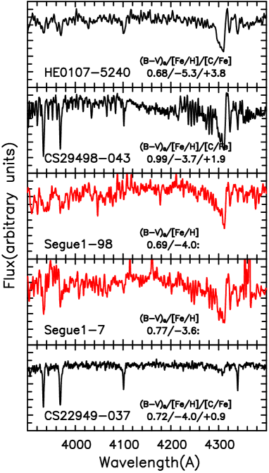
Figure 10: Comparison of the spectra of the putative C-rich stars Seg 1–7 and Seg 1–98 with those of extremely Fe-poor, C-rich Galactic halo giants of similar color ($T_{\rm eff}$) (from ANU’s 2.3m telescope). The spectra have been continuum-normalized and broadened to resolution of FWHM = 2.5 Å. Individual panels list (B-V)₀/[Fe/H]/[C/H], as indicated, from Aoki et al. (2002), Christlieb et al. (2004), McWilliam et al. (1995), and the present work.

For the Segue 1 candidates, we shall consider here only those stars having spectra with more than 200 counts per 0.34 Å pixel at 4150 Å and velocities in the range 185–230 km s^-1 following the discussion in Section 3.1.2. The data for the five Segue 1 candidates that meet these criteria are given in the first five rows of Table 4 (which has the same column structure as Table 3). Their spectra are presented in Figure 9 over the wavelength range 3900–4400 Å. One sees immediately that these spectra are not what one might have expected for a sample of objects taken from a stellar system with a monomodal abundance distribution. Two things are obvious. First, there is a large range in the strength of the G-band at 4300 Å; and second, the Ca II H & K lines (at 3968 Å and 3933 Å) differ widely from star to star within the group. In particular, Seg 1–7 and Seg 1–98 have weak and somewhat ill-defined Ca II lines and very strong G-bands. Such behavior is not unprecedented in extremely metal-poor stars of the Galactic halo. Figure 10 compares the spectra of these two stars with those of the halo, extremely metal-poor, C-rich giants CS22949–037, CS29498–043, and HE0107–5240 (obtained with the Double Beam Spectrograph on ANU’s 2.3m telescope on Siding Spring Mountain), which collectively have –5.4 $<$ [Fe/H] $<$ –3.8 and 0.9 $<$ [C/Fe] $<$ 3.8 (McWilliam et al. 1995; Aoki et al. 2002; Christlieb et al. 2004). One consequence of the apparent carbon-richness of the two Segue 1 objects is that the contamination by CH lines in the region of the Ca K line may lead to erroneously overestimated iron abundances derived from the K line on low resolution spectra (see e.g. Christlieb et al. 2002; Frebel et al. 2005; and Beers & Christlieb 2005).

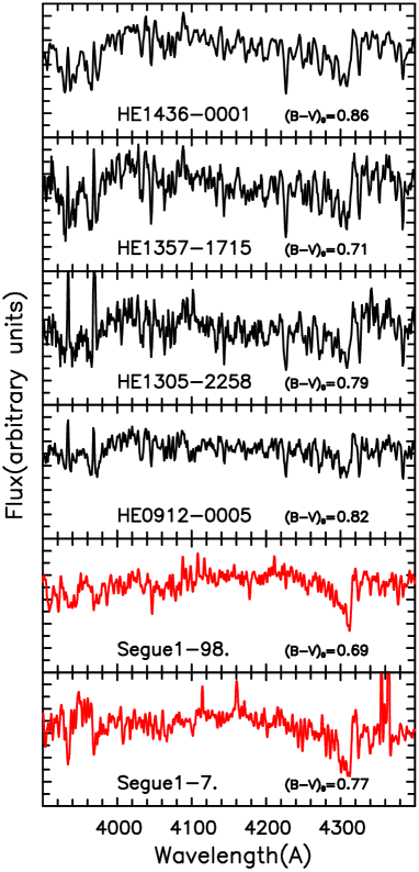
Figure 11: Comparison of the spectra of Seg 1–7 and Seg 1–98 with those of extremely metal-poor stars from the Hamburg ESO Survey found serendipitously to have Ca II H&K emission cores. See text for discussion.

There are also two mundane explanations of the weak Ca II lines in Seg 1–7 and Seg 1–98 that one should consider. The first is that the effect is due to the relatively low $S/N$ of our spectra. The second is that both stars are high-velocity (V_r $\sim$ 200 km s^-1) stars with Ca II H & K lines that have emission cores. We searched our collection of some 3000 medium resolution (FWHM $\sim$ 2.5 Å) spectra of Hamburg ESO Survey (HES) metal-poor candidates (see Norris et al. 2007) for stars that have weak Ca II H & K lines as the result of core emission, and found some 10 objects with relatively weak H & K emission leading to weak overall H & K line absorption. In Figure 11 we compare the spectra of Seg 1–7 and Seg 1–98 with four of these objects. There is clearly not a good match between the spectra of the HES stars and those of the candidate Segue 1 stars. However, one might imagine that if in the candidate Segue 1 stars there were weaker emission features than those seen in the HES stars in Figure 11 the abundances we derived for the candidate Segue 1 stars could be erroneous.

5 ATMOSPHERIC PARAMETERS

To determine relative carbon abundances ([C/Fe]) in what follows, we shall also need the atmospheric parameters effective temperature ($T_{\rm eff}$), surface gravity (log $g$), and metal abundance ([M/H]), where for simplicity we shall assume [M/H] = [Fe/H]. In Tables 3 (for Boötes I) and 4 (for Segue 1) we present data that we have used for this purpose. Columns (4)–(6) contain $ugriz$ photometry for $g$, $(g-r)_{0}$, and $(r-z)_{0}$ from Data Release 7 of the Sloan Digital Sky Survey (Abazajian et al. 2009), where the colors have been corrected for reddenings corresponding to E$(B-V)$ = 0.02 (Belokurov et al. 2006) and 0.032 (Geha et al. 2009), for Boötes I and Segue 1, respectively. From our spectra of the Segue 1 objects in Table 4, we measured values of the Ca II K line-strength index, K^′, defined by Beers et al. (1999), which are presented in column (7) of Table 4. For Boötes I, K^′ values from Norris et al. (2008) are included in column (7) of Table 3.

As described in Norris et al. (2010), $T_{\rm eff}$ and log $g$ can be estimated for metal-poor red giants in dSph systems by using $ugriz$ photometry together with the synthetic $ugriz$ colors of Castelli and the Yale–Yonsei (YY) Isochrones (Demarque at al. 2004) with an age of 12 Gyr, and the assumption that the stars lie on the red giant branch of the system.

For the Boötes I and Segue 1 stars investigated here, values of $T_{\rm eff}$ and log $g$ were obtained for each of $(g-r)_{0}$ and $(r-z)_{0}$, and also $(B-V)_{0}$ (see below). A check on these atmospheric parameters was obtained by using a technique similar to that described by Norris et al.  in which the absolute magnitude M_V – derived from the apparent magnitude and distance modulus of the parent system – replaces color, together with the adoption of the Yale-Yonsei Isochrones and the assumption that the stars lie on the red giant branch of the parent dSph. To determine the estimated values of absolute visual magnitude M_V, we used the Lupton (V, $g$)– transformation, together with our adopted reddening, the distance moduli of Martin et al. (2008), and the assumption A_V = 3 $\times$ E($B-V$). Then, for the YY isochrone of assumed abundance [Fe/H] (and the above age of 12 Gyr), by interpolation in the ($T_{\rm eff}$, M_V)– and (log $g$, M_V)– relationships defined by the isochrone we determine the values of $T_{\rm eff}$ and log $g$ corresponding to the derived value of M_V. Agreement between the atmospheric parameters obtained from $ugriz$ colors with those from absolute magnitude for Boötes I was excellent: for the 16 stars in Table 3 we obtained average differences $\langle$$\Delta$$T_{\rm eff}$$\rangle$ = 70K and $\langle$$\Delta$log $g$$\rangle$ = 0.2. For Segue 1, on the other hand, the agreement was considerably poorer, with $\langle$$\Delta$$T_{\rm eff}$$\rangle$ = 230K and $\langle$$\Delta$log $g$$\rangle$ = 0.5. If, however, we exclude Seg 1–42, the hottest star in the sample, and for which the two $T_{\rm eff}$ and log $g$ estimates differ by 440K and 0.9 dex respectively, we obtain $\langle$$\Delta$$T_{\rm eff}$$\rangle$ = 140K and $\langle$$\Delta$log $g$$\rangle$ = 0.4. We shall return to this point below, once we have discussed the abundances of the putative Segue 1 members.

Metal abundances were determined in two ways. First, we used the calibration of Beers et al. (1999), which permits one to determine [Fe/H], given observed values of K^′ and (B–V)₀. In order to do this, we determined (B–V)₀ from the values of $(g-r)_{0}$ in Tables 3 and 4. For stars with $(g-r)_{0}$ $>$ 0.545 (corresponding to $(B-V)_{0}$ $>$ 0.7), we adopted the transformation $(B-V)_{0}$ = 1.197$\times$$(g-r)_{0}$ + 0.049, appropriate for metal-poor red giants, following Norris et al. (2008). This applied for all but two objects (Seg 1–31 and Seg 1–42), for which we adopted $(B-V)_{0}$ = 0.916$\times$$(g-r)_{0}$ + 0.187, from Zhao & Newberg (2006), valid for metal poor-stars over the range –0.15 $<$ $(g-r)_{0}$ $<$ 0.55.

The second method of abundance determination involves model atmosphere analysis of high-resolution, high $S/N$, spectra obtained with VLT/UVES (Norris et al. 2010, for Boo$-$1137), and with VLT/UVES/Flames for a further seven of the Boötes I stars, which will be reported elsewhere (Gilmore et al. 2010 in prep.).

The atmospheric parameters for Boötes I and Segue 1 are presented in Table 3 and 4, where columns (8)–(9) contain $T_{\rm eff}$ and log $g$ obtained from colors as described above, while column (10) presents [Fe/H] (except for Seg 1–7 and Seg 1–98), based on the above two methods, where the tabulated abundance gives precedence to the UVES based value if available, failing which the AAOmega K^′-based result is used.

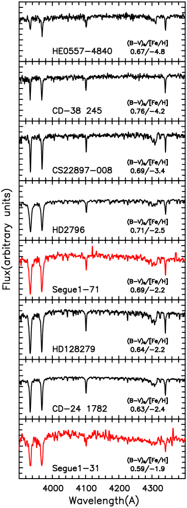
Figure 12: Comparison of the spectra of the C-normal Segue 1 stars with C-normal Galactic halo giants of similar color ($T_{\rm eff}$) (from ANU’s 2.3m telescope). The spectra have been continuum-normalized and broadened to resolution of FWHM = 2.5 Å. Individual panels list (B-V)₀/[Fe/H] from Cayrel et al. (2004), Chiba & Yoshii (1998), and Norris et al. (1985), as described in the text.

Our abundances for Segue 1 deserve comment. For Seg 1–31 and Seg 1–71, we derive relatively high values of [Fe/H] = –1.9 and –2.2, respectively. To give the reader a feeling for the case for the high abundances of these objects, we compare their spectra in Figure 12 with those of Galactic halo giants having similar colors, and abundances in the range –4.8 $<$ [Fe/H] $<$ –2.2. (The colors of the Galactic stars are taken from Cayrel et al. (2004), Norris, Bessell, & Pickles (1985), and Norris et al. (2007), while their abundances come from Cayrel et al. (2004), Chiba & Yoshii (1998), and Norris et al. (2007).) Examination of the spectra, in the region of the Ca II H & K lines (3900–4000 Å), clearly supports our relatively high abundances. That said, we recall that Geha et al. (2009) have reported a red giant in Segue 1 (their star 3451364) with [Fe/H] = –3.3. We note then that the Segue 1 spectra in Figure 12 have much stronger Ca II H & K lines than seen in CS22897–008 (in the third panel from the top), which has [Fe/H] = –3.4, similar to the abundance of the Geha et al. star. Said differently, there appears to exist a large abundance range ($\Delta$[Fe/H] $\sim$ 1 dex) within the sample of candidate members of Segue 1.

The abundances of the more-enriched candidate members of Segue 1 are, however, close to that of a typical field halo star at the distance of Segue 1 (the outer halo of Carollo et al. 2007). Further, there are clear indications of an abundance gradient from the core of the Sgr dSph to its tidal streams, with a mean metallicity [Fe/H] $\sim$ –1 derived from M giants (at heliocentric distances greater than $\sim 10$ kpc; Chou et al. 2007) and –1.8 from RR Lyrae stars in the leading arm, at heliocentric distances of $\sim 50$ kpc (Vivas, Zinn, & Gallart 2005). These results suggest that at [Fe/H] $\sim$ –1.5 – –2, both field halo stars and Sgr debris would be hard to distinguish from members of Segue 1, given that some models of the Sgr streams predict similar velocities (e.g. Niederest-Ostholt et al. 2009).

For the two putative C-rich objects in Segue 1, we also derived [Fe/H] using the Beers et al. (1999) formalism, which leads to ${\rm[Fe/H]=-3.6}$ and –4.0 for Seg 1–7 and Seg 1–98, respectively. At this stage we regard these values as uncertain for the reasons discussed in Section 4. We shall defer further discussion of them until Section 6.

It is somewhat difficult to estimate realistic errors for $T_{\rm eff}$ and log $g$ that include both internal and potential external errors. The cited errors in the DR7 $ugriz$ colors propagate to relatively small errors in $T_{\rm eff}$ and log $g$, and it is probably more realistic to concentrate on systematic effects. One measure of this could be the internal spread in the results of the three methods based on calibrations of $(g-r)_{0}$, $(r-z)_{0}$, and $(B-V)_{0}$ described above. We find that the averages of the standard error of the mean for the 16 Boötes I objects in Table 3 are $\langle$$\Delta$$T_{\rm eff}$$\rangle$ = 40K and $\langle$$\Delta$log $g$$\rangle$ = 0.1. These are somewhat smaller that the average differences of $\langle$$\Delta$$T_{\rm eff}$$\rangle$ = 70K and $\langle$$\Delta$log $g$$\rangle$ = 0.2 obtained above from colors and absolute magnitude (i.e. assuming that the stars are indeed red giants at the distance of Segue 1). We adopt the larger differences as error estimates in what follows. For the five Segue 1 stars we find average differences of $\langle$$\Delta$$T_{\rm eff}$$\rangle$ = 90K and $\langle$$\Delta$log $g$$\rangle$ = 0.2; and if we exclude Seg 1–42, the problematic star discussed above, these values become $\langle$$\Delta$$T_{\rm eff}$$\rangle$ = 100K and $\langle$$\Delta$log $g$$\rangle$ = 0.3.

We now return to the issue of the discrepant values of $T_{\rm eff}$ and log $g$ obtained above for Seg 1–42 from estimates based on color and absolute magnitude. While this object appears to be the hottest of the stars in Table 4, it is also the most metal-rich, with [Fe/H] = –1.5. Given that this is fundamentally at odds with basic concepts of evolution on the red giant branch (more metal-rich stars should be cooler), and our assumption that Seg 1–42 lies on the giant branch of Segue 1, we shall exclude Seg 1–42 from further consideration, on the assumption it is not a red giant member of Segue 1. In what follows we shall adopt mean errors of $\sigma$($T_{\rm eff}$) = 140K and $\sigma$(log $g$) = 0.4 for the four remaining candidate Segue 1 giants, the larger of our two estimates obtained when we exclude Seg 1–42 from consideration. We note parenthetically here that the differences between our two methods of deriving atmospheric parameters are commensurate, to within these errors, with the assumption that the other stars in Table 4 lie on the RGB of Segue 1.

Abundance errors for Boötes I are $\sigma$[Fe/H] = 0.35 for data obtained with AAOmega (Norris et al. 2008) and $\sigma$[Fe/H] = 0.15 for the results from VLT/UVES and VLT/Flames/UVES (Norris et al. 2010; Gilmore et al. 2010 in prep.). For Seg 1–31 and Seg 1–71 we adopt $\sigma$[Fe/H] = 0.4.

6 FURTHER ASSESSMENT OF THE PUTATIVE SEGUE 1 C-RICH, EXTREMELY METAL-POOR STARS

It is difficult to over-emphasize the implications of Segue 1 membership of the two C-rich, extremely metal-poor candidates Seg 1–7 and Seg 1–98. Put most simply, C-rich stars, having [Fe/H] $\lesssim$ –3.3 are extremely rare: few are known, and only some seven have been analyzed in detail. The existence of such objects in the ultra-faint dwarfs would have strong implications for these systems being building blocks of the Galaxy’s outer halo.

After the analysis reported here was complete, we sought to obtain high-resolution, high $S/N$ data for both Seg 1–7 and Seg 1–98. There were two significant developments. First, Evan Kirby and Joshua Simon informed us that they have near-infrared spectra for Seg 1–98 that yield much higher values of [Fe/H] than suggested here, and generously permitted us to examine several of their spectra. We accept their argument, and shall not consider that object further in this paper. Further data are needed to clarify the inconsistency.

Second, in April 2010, we obtained spectra taken with VLT/UVES of Seg 1–7 with resolution R = 35,000, and $S/N$ = 40/0.027 Å pixel at 4300 Å. We shall report the analysis of these data at a later time. Suffice it here to say that our preliminary analysis yields a radial velocity of 204.3 $\pm$ 0.1 km s^-1 (internal error), while for atmospheric parameters $T_{\rm eff}$ = 4960K and log $g$ = 1.9 (from Table 4), and using techniques described in Norris et al. (2010), our preliminary analysis yields [Fe/H] = –3.5, and [C/Fe] $\sim$ +2.5 for this object. We shall retain Seg 1–7 in our analysis, and list this value of [Fe/H] (which agrees well with that reported in the previous section) in Table 4. Finally, for completeness and the discussion that follows, we also include the data of Geha et al. (2009) for their red giant 3451364 in the final row of Table 4.

7 CARBON ABUNDANCES

AAOmega spectra of the Boötes I members in Table 3 were presented in the wavelength range 3900–4400 Å in Figure 1 of Norris et al. (2008), to which we refer the reader. In that figure one sees a clear and relatively large range in the strength of the G-band (of the CH molecule) at 4300 Å. We analyze these band strengths below to determine carbon abundances.

Using the atmospheric parameters in Tables 3 and 4, we have computed (1D/LTE) model atmosphere synthetic spectra in the region of the G-band 4270–4335 Å using the procedures described by Stanford et al. (2007, and references therein), to which we refer the reader for details. Suffice it here to say that the spectrum synthesis code was that of Cottrell & Norris (1978), the models used were those of Kurucz (1993), and the CH $gf$ values of Kurucz were modified by 0.5 dex to provide a fit between the observed and synthetic model atmosphere spectrum of the Sun. As a further test of the procedure, we determined the relative carbon abundance for the archtypical metal-poor red giant HD 122563 using the observed spectrum and atmospheric parameters ($T_{\rm eff}$ = 4650K, log $g$ = 1.4, [Fe/H] = –2.7) of Ryan et al. (1996) and adopting [O/Fe] = +0.6. The value obtained was [C/Fe] = –0.35, in good accord with the value of –0.4 reported by Sneden (1973) and by Cayrel et al. (2004).

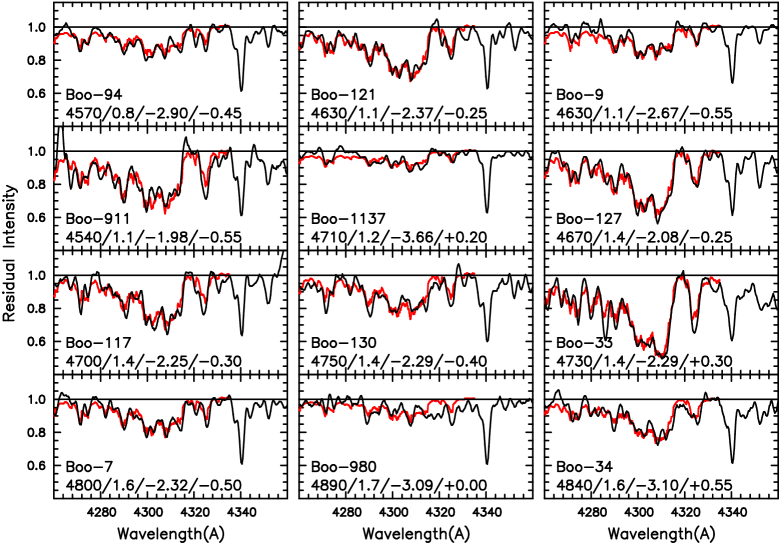
Figure 13: Comparison of the observed spectra (black lines) of 12 red giants in Boötes I with the best fitting synthetic spectra (red lines) in the region of the G-band of the CH molecule. The stellar identification and T_eff/log $g$/[Fe/H]/[C/Fe] are presented in each panel. (The corresponding spectra of the stars in the range 3900–4400 Å may be found in Figure 1 of Norris et al. (2008).)

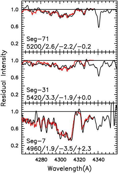
Figure 14: Comparison of the observed spectra (black lines) of the three putative radial velocity members of Segue 1 with the best fitting synthetic spectra (red lines) in the region of the G-band. Stellar identification and T_eff/log $g$/[Fe/H]/[C/Fe] are presented in each panel.

The fits of the synthetic spectra to the present observations are shown in Figure 13 for Boötes I, for the 12 stars in Figure 1 of Norris et al. (2008) (there presented over the larger range 3900–4400 Å) and in Figure 14 for Segue 1. The derived abundances, [C/H], are presented in column (11) of Tables 3 and 4. Their accuracy is estimated to be ${\Delta}$[C/H] = 0.2 and 0.4, for Boötes I and Segue 1, respectively, which include the propagation of errors in the atmospheric parameters $T_{\rm eff}$, log $g$, and [Fe/H] given in Section 5 above (of which the first is the most significant), and the fitting error. [C/H] for Boo$-$1137 in Table 3 has also been determined by Norris et al. (2010) using high-resolution, high $S/N$ VLT/UVES spectra, interpreted using the MOOG code of Sneden 1973) (see Norris et al. 2010 for details) and the models of Castelli & Kurucz (2003; http://wwwuser.oat.ts.astro.it/castelli/grids.html). They determined [C/H] $=-3.41$, in good accord with the value of [C/H] = –3.46 in Table 3.

8 ABUNDANCE SPREADS AND DISTRIBUTIONS

8.1 Carbon Abundances in the Dwarf Spheroidal Galaxies of the Milky Way

8.1.1 The Spread of [C/H] in Boötes I and Segue 1

The first conclusion of our investigation is that the spread of carbon abundance in both Boötes I and Segue 1 is large. For the former, four of the 16 objects in Table 3 have [C/H] $\lesssim$ –3.1, while two have [C/H] $\gtrsim$ –2.3, suggesting a range of $\Delta$[C/H] $\sim$ 0.8. In Table 4 one finds that for Segue 1 there exists a range $\Delta$[C/H] $\sim$ 1.0. These results are relatively robust to errors in the atmospheric parameters assumed in the analysis: for example, representative errors of $\Delta$$T_{\rm eff}$ = 100K, $\Delta$log $g$ = 0.3, and $\Delta$[Fe/H] = 0.3, cause errors in [C/H] of 0.2, 0.1, and 0.0, respectively. (The ranges in [C/Fe] in Boötes I and Segue 1 $\Delta$[C/Fe] are $\sim$ 1.0 and $\sim$ 2.5, respectively. We discuss the dispersion in [C/Fe] below.)

8.1.2 Relative Carbon Abundance, [C/Fe], as a Function of Metallicity and Absolute Magnitude

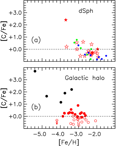
Figure 15: [C/Fe] as a function of [Fe/H] for Galactic dwarf satellite (upper panel) and halo (lower panel) red giants. In the upper panel the ultra-faint Boötes I and Segue 1 are represented by open and filled red stars, respectively, while the filled green and blue circles come from Frebel et al. (2010a) for the ultra-faint UMa II and Com, and from Cohen & Huang (2009) for the Draco dSph, respectively. The open and filled red circles in the lower panel represent the “mixed” and “unmixed” stars of Spite et al. (2005), while the filled black symbols represent the C-rich extremely iron-poor giants HE0107–5240 ([Fe/H] = –5.40, Christlieb et al 2004), HE0557–4840 ([Fe/H] = –4.75, Norris et al. 2007), CS22949–037 ([Fe/H] = –3.97, Spite et al. 2005), CS29498–043 ([Fe/H] = –3.75, Aoki et al. 2002) and CS22957–027 ([Fe/H] = –3.38, Norris et al. 1997).

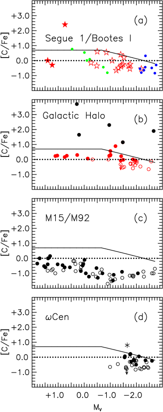
Figure 16: The dependence of [C/Fe] on absolute magnitude, M_V, for (a) the ultra-faint Boötes I and Segue 1 (open and filled stars), respectively, and UMa II and Com (filled green circles) from Frebel et al. (2010a), together with data from Cohen & Huang (2009) for the Draco dSph (filled blue circles), (b) extremely metal-poor giants of the Galactic halo (symbols as in Figure 14), (c) the globular clusters M15 (open symbols) and M92 (filled symbols; from Langer et al. 1986 and Trefzger et al. 1983), and (d) $\omega$ Cen, where filled and open circles refer to CO-strong and CO-weak stars, respectively, and the asterisk stands for a CH star (from Norris & Da Costa 1995). The horizontal dotted line lies at the solar value, [C/Fe] = 0.0, while the continuous line corresponds to the division of Aoki et al. (2007) between C-rich and C-normal stars. See text for discussion.

In Figure 15 we compare the behavior of relative abundance [C/Fe] as a function of [Fe/H] for Boötes I, Segue 1, other dwarf systems, and for the Galactic halo. In the upper panel the open and filled stars represent red giants in Boötes I and Segue 1, respectively, while the filled green circles stand for stars in the ultra-faint dwarfs UMa II and Com from Frebel et al. (2010a) and the filled blue ones for stars in the more luminous Draco dSph (from Cohen & Huang (2009). The lower panel presents results for red giants in the Galactic halo taken from Spite et al. (2005), where open and filled red circles denote their “mixed” and “unmixed” stars. As we shall see in Figure 16 the incidence of “mixed” stars increases with increasing luminosity. Filled black circles represent stars with large enhancements of C and N (and often O) from Aoki et al. (2002), Cayrel et al. (2004), Christlieb et al. (2004), Norris, Ryan, & Beers (1997), and Norris et al. (2007) (see the figure caption for identifications). While there is a clear similarity between the two panels, some caution is warranted. The sample in the lower panel of the figure is not unbiased. Of the 39 objects plotted, 30 come from the HK survey (Beers, Preston, & Shectman 1992), two from the HES (HE0107–5240 (Christlieb et al. 2004) and HE0557–4840 (Norris et al. 2007), both with [Fe/H] $<$ –4.4), and five from brighter miscellaneous sources (all with [Fe/H $>$ –3.0). There have been strenuous endeavors to observe all stars in the HK survey with [Fe/H] $<$ –3.0: to our knowledge, as a result of this comprehensive effort, some 35 of the red giants in the HK survey in the range –4.2 $<$ [Fe/H] $<$ –3.0 now have high quality abundance analyses, 23 of which appear in Figure 15. Given the fact that Spite et al. (2005) chose to observe stars with [Fe/H] $<$ –2.5, the data in the lower panel are therefore very incomplete above that limit. In contrast, the two HES stars in the figure, with [Fe/H] $<$ –4.4, represent only the (extremely important) low abundance tail of the HES distribution.

Figure 16 presents the behavior of [C/Fe] as a function of absolute visual magnitude, M_V. The upper panel (a) presents results for the red giants in Boötes I, Segue 1, and dwarf galaxies as defined in Figure 15, while panels (b)–(d) contain data for three other stellar populations of the Milky Way. Panel (b) presents giants of the Galactic halo (the sample presented in Figure 15. Note that the incidence of “mixed” stars of Spite et al. (2005) (the open symbols) increases as one moves to higher luminosity, consistent with the interpretation of increased importance of mixing as the star ascends the giant branch, crossing the “red giant branch bump” (see Gratton et al. 2000). Panel (c) contains giants in the globular clusters M15 (open circles) and M92 (filled circles) (Langer et al. 1986; Trefzger et al. 1983), both of which have [Fe/H] $\sim$ –2.2, with little or no internal dispersion in iron abundance. Finally, (d) presents results for the brightest giants in the Galaxy’s most massive and chemically inhomogeneous globular cluster $\omega$ Centauri (from the chemically biased sample of Norris & Da Costa 1995, hereafter ND). (Open and filled circles refer to CO-weak and CO-strong objects (of which more below), while the asterisk represents a CH star.) $\omega$ Cen has been proposed to have once been the core of a nucleated dwarf galaxy, captured long ago by the Milky Way (see Bekki and Freeman 2003, and references therein) so that the spread of chemical abundances reflects evolution within the deeper potential well of the host galaxy (e.g. Bekki and Norris 2006; Marcolini et al. 2007). If, alternatively, $\omega$ Cen itself possessed a high enough baryonic mass to retain some ejecta from evolved stars and supernovae (e.g. Norris et al. 1996; Gnedin et al. 2002) it is simply another example of a self-enriching system and would be expected to show similar scalings to those of the dwarf galaxies. We favor this second model below.

One sees a large range of [C/Fe] in these panels. For heuristic purposes we also show the continuous line corresponding to the division of Aoki et al. (2007) between C-rich and C-normal stars of the Galactic halo, taking account of mixing, and associated carbon reduction, as stars ascend the RGB.

8.1.3 Red Giants as Probes of Galactic Carbon Enrichment

The data in Figure 16 encapsulate the difficulties one encounters in seeking to interpret the observed carbon abundances of red giants in the old stellar populations of the Milky Way system in terms of galactic chemical enrichment. Not only must one understand the yields of the supernovae that enriched successive stellar generations; one must also deal with the poorly understood effects of evolutionary mixing that occurs as old stars ascend the red giant branch.

It is difficult to see how the results for M15 and M92 in Figure 16(c), where [C/Fe] decreases as one moves up the giant branch – accompanied by increasing [N/Fe] (Langer et al. 1986, and references therein) – can be explained in any other way than by evolutionary mixing involving the CN-cycle (see e.g. Langer et al. 1986), superimposed on the carbon abundance profile of the protosystems from which these clusters formed. M15 and M92 have [Fe/H] $\sim$ –2.2, which lies within $\Delta$[Fe/H] = 0.3 dex of the mean abundance of Boötes I. Why then do the Galactic field halo stars and the Boötes I stars in Figure 16(a) not share the extreme evolutionary mixing signature of low carbon on the upper giant branch that one sees for M15 and M92 (Figure 16(c))? One obvious difference that distinguishes the giants of a given globular cluster is their small age range, which is essentially zero, while there is no reason to assume this holds for either the Galactic halo or Boötes I. That said, it remains unclear why this should produce the above abundance differences.

8.1.4 Similarities between the [C/Fe] Distributions of the Ultra-Faint Dwarf Galaxies and the Galactic Halo

The above caveats concerning evolutionary mixing effects notwithstanding, consideration of Figure 15 and the upper two panels of Figure 16 suggests a strong similarity between the carbon abundance distributions of the red giants of the Galaxy’s dwarf galaxies and halo. At first glance it might also appear that the available data for the brighter giants in $\omega$ Cen share this similarity. Given, however, the biased nature of the ND sample introduced by their selection towards the chemical extremes of the cluster, such a conclusion would be premature. All one can say is that at least some stars in $\omega$ Cen show abundance patterns like those of the halo and Boötes I.

If one accepts that the carbon abundance signatures of the Galaxy’s dwarf galaxies and halo are essentially the same, and the conclusion of Spite et al. (2005) that giants with [Fe/H] $\lesssim$ –2.5 comprise “mixed” and “unmixed” stars, with the “unmixed” group “reflecting the abundances of the early Galaxy”, one might suggest this could well apply also to the ultra-faint dwarfs. The hypothesis is testable. According to Spite et al. (2005, see their Figures 6–8) the “mixed” stars have low C and high N (consistent with dredge up of CNO processed material), together with strong Li dilution, while the “unmixed” objects show no evidence for C to N conversion, and only moderate Li depletion. More data to determine nitrogen and lithium abundances in the dwarf galaxies are clearly needed to address the question.

Regardless of whether or not the abundances have been modified by stellar evolutionary effects, the data in the upper panel of Figure 15 show that the present relative carbon abundances [C/Fe] of stars in the Galaxy’s ultra-faint dwarf satellites are similar to those of stars in its halo, and in the range –3.5 $<$ [Fe/H] $<$ –2.5 has the value [C/Fe] $\sim$ 0.3.

8.2 Metallicity Distribution Functions

8.2.1 Boötes I

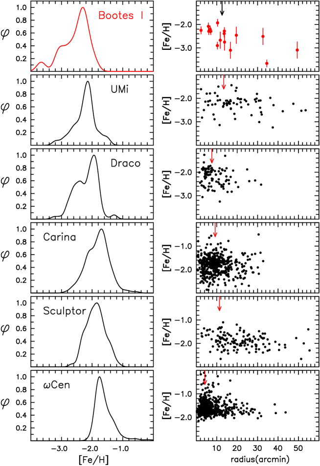
Figure 17: Left: Metallicity distribution functions for Boötes I and Galactic dwarf spheroidal satellites. Right: [Fe/H] vs elliptical radial distance for Boötes I and the other systems shown in the left panels (except for $\omega$ Cen, for which radial distance is plotted). The arrows on the upper x-axes indicate the position of half-light radius. For the other systems, the data have been taken from Winnick (2003, UMi and Draco), Koch et al. (2006, Carina), Battaglia et al. (2008, Sculptor), and Norris et al. (1996, $\omega$ Cen).

Accurate iron abundances are now available for 16 radial-velocity candidate members of Boötes I, and if we restrict this to those within 2.5r_h (at which radius, adopting the surface brightness of Martin et al. (2008), the probability of membership is 0.20 of its value at r_h), this number decreases to 15. The outlier, Boo–980, lies at 3.9r_h and has [Fe/H] = –3.1, rather suggestive of membership. The upper panels of Figure 17 then present the metallicity distribution function (MDF) (left panel) and the dependence of [Fe/H] versus elliptical radius (right panel) for all 16 Boötes I stars, while the lower panels show the results for Galactic dSph systems and $\omega$ Cen (where, for the latter, radial distance is employed in the right panel). To improve their formal accuracy, we replaced the Boötes I AAOmega abundances for Boo–7, 121, and 911 presented in Table 3, for which we have no high-resolution abundances, with values from Feltzing et al. (2009). There are three points to note about Boötes I. First, in comparison with the steep rise in the MDF seen in $\omega$ Cen between [Fe/H] = –2.2 and –1.8, its MDF has a slow increase from lowest abundance to the MDF peak, covering [Fe/H] = –3.7 to –2.3, similar to that seen in the dSphs, with recent dSph abundance results only accentuating the low metallicity tails to their MDFs; second, of the dSph systems with published data for individual stars, it has the highest percentage of objects with [Fe/H] $<$ –3.0; and third, while there are too few objects to permit a strong statement, it appears to have a (marginally significant with these data) radial abundance gradient. Such a gradient is seen in some of the other dSph systems, as reported by Winnick (2003), Tolstoy et al. (2004), and Koch et al. (2006).

8.2.2 Segue 1

We noted in Section 1 that Geha et al. (2009) provided the first spectroscopic abundance estimate for Segue 1. They analyzed a single radial-velocity member (their star 3451364, with velocity 215.6 km s^-1, 9.5 km s^-1 larger than the systemic velocity), and assuming it to be a red giant reported [Fe/H] = –3.3 $\pm$ 0.2, based on spectrum synthesis in the CaT wavelength ($\sim$ 8300–8700 Å) region. As discussed in Sections 4–6, we have three objects with reliable abundances and radial velocities consistent with membership of the Segue 1 system, and one other velocity candidate (Seg 1–98) with inconsistent blue and red abundance estimates. Of these four stars, two (Seg 1–31 and Seg 1–71) are relatively metal rich ([Fe/H] $\sim$–2.0), while the C-rich star Seg 1–7 is extremely metal-poor, with [Fe/H] = –3.5. These four velocity member stars may still, statistically, include a chance non-member. It is thus probable, but not certain, that there exists a large [Fe/H] range in the Segue 1 system. Clearly, four objects are too few to say much about the MDF, other than to reiterate our earlier statement that this system, at face value, is not monometallic. Additionally, there remains the open question of whether we are looking at an ultra-faint dwarf (Geha et al. 2009), tidal debris from the Sgr dSph (Niederste-Ostholt et al. 2009), or a mixture of both.

8.2.3 Comparison of metallicity means and dispersions with those of other Milky Way dwarf galaxies

Kirby et al. (2008) first reported that the mean metallicity of dwarf galaxies continues to decrease as one proceeds from the more luminous dSphs to the low absolute magnitudes of the ultra-faint systems. We discuss here how our results for Boötes I and Segue 1 compare with their relationship, and also investigate the behavior of metallicity dispersion, $\sigma$([Fe/H]).

In Table 5 we present mean metallicities, $\langle$[Fe/H]$\rangle$, and dispersions about the mean $\sigma$([Fe/H]) (i.e. standard deviations) for Milky Way dwarf satellites and the chemically inhomogeneous globular cluster $\omega$ Cen, together with other data and their sources. Columns (1)–(3) contain identification, absolute visual magnitude M${}_{V,\,total}$ and its source, (4)–(5) present mean metallicity and its error, (6)–(7) the abundance dispersion and its error, and (8)–(9) give the number of stars in each sample and the sources of the abundance data. In compiling the table we chose abundance determinations that met the following criteria: (1) the observed stars were chosen without chemical bias, which could result, for example, if selection were biased toward the color extremes in the CMD in an effort to sample the abundance extremes of the system and (2) first preference was given to investigations that determined [Fe/H] from observations that included features of Fe as a primary observable. In determining uncertainties in the abundance dispersions, we followed the precepts of Da Costa et al. (1977), which explicitly remove the effects of instrumental and statistical abundance errors in the determination of dispersion. For Boötes I, we used the data in Table 3, to which we assign measurement errors of 0.15 dex for the ten high-resolution analyses (including the three Feltzing et al. (2009) stars discussed in Section 7.1), on the one hand, and 0.35 dex for the six remaining AAOmega-based result, on the other, while for the Segue 1 objects we adopted $\Delta$[Fe/H] = 0.4 dex for Seg 1–31 and Seg 1–71) and 0.2 dex for the Geha et al. red giant and Seg 1–7. For the other systems we assumed abundance errors of 0.2 dex for the ultra-faint dwarfs, UMi, and Draco (based on error estimates in Kirby et al. (2008) and data of Winnick (2003)), and 0.10 dex for the other dSphs and $\omega$ Cen (following Battaglia et al. (2008), Helmi et al. (2006), and Norris et al. (1996)).

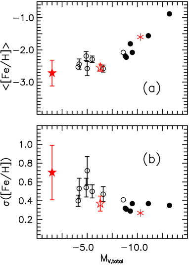
Figure 18: (a) Mean metallicity, $\langle$[Fe/H]$\rangle$, and (b) metallicity dispersion, $\sigma$[Fe/H], versus system absolute magnitude, M${}_{V,\,total}$, for the dwarf galaxy satellites of the Milky Way and $\omega$ Cen. The filled and open circles refer to values for the dSphs and ultra-faint dwarf galaxies from the literature, respectively while the open and filled stars represent Boötes I and Segue 1, respectively, from the present work. The parameters for Segue 1 assume all four stars discussed in the text (Seg 1–7, 31, 71, and 3451364) are indeed members. $\omega$ Cen is shown as the asterisk. See Table 5 for data and their sources. Error bars are not plotted when they are smaller than 0.10 and 0.05 for $\langle$[Fe/H]$\rangle$ and $\sigma$[Fe/H], respectively.

Figure 18 presents mean metallicities and dispersions about the mean as a function of integrated absolute visual magnitude M${}_{V,\,total}$. Inspection of the figure shows the continued decrease in mean [Fe/H] as one proceeds to lower absolute magnitude, first reported by Kirby et al. (2008), together with an apparent increase in the abundance dispersion. Whether or not this trend continues to the luminosity of Segue 1 is uncertain, being sensitive to membership assignments. The two Segue 1 stars with [Fe/H] $\sim$ –2. may be field interlopers. The two very metal-poor stars are offset in either velocity (Seg 1–3451364) or position (Seg 1–7) from the reported systemic values. More data are clearly required for Segue 1 to test this suggestion more rigorously. That said, an increased abundance spread is intuitively consistent with inhomogeneous stochastic enrichment in very low-baryonic-mass and low-metallicity systems, enriched by very few supernova events.

8.3 The Carbon-Rich, Extremely-Metal-Poor Star in Segue 1

Seg 1–7 has a spectrum that is similar to those of the C-rich, extremely-metal poor stars of the Galactic halo. As emphasized above, more work is needed to investigate the possible connection between the parent populations of the Galaxy’s dwarf satellites and halo. The question is an important one for an understanding of chemical enrichment at the very earliest times. As one proceeds to lowest abundance in the Galactic halo (i.e. to the oldest stars) one finds that the fraction of C-rich objects increases – indeed all stars to date with [Fe/H] $\lesssim$ –4.3 are C-rich (see e.g. Norris et al. 2007). Further, efforts to understand the intriguing relative abundance distributions of C-rich stars with [Fe/H] $\lesssim$ –3.5, many of which are characterized by enhanced values of some, or all, of [C/Fe], [N/Fe], [O/Fe], and [Mg/Fe] of order 1–2 dex, have led to the proposal of severely non-canonical supernovae at the earliest times and lowest metallicities, involving for example “mixing and fallback” during explosion (see Iwamoto et al. 2005, and references therein). While it has been proposed that the elemental abundances of the most metal-poor stars in the field halo can be explained by the explosions of zero-metallicity massive stars with a Salpeter IMF over the range 15–40M_⊙ (Joggerst et al. 2010), we note that these objects do not produce the extreme CNO abundances of a significant fraction of CEMP stars with [Fe/H] $<$ –3.5. If more exotic supernovae are a natural feature of the evolution of extremely metal-poor massive stars, they may have also left their signatures in the lowest abundance stars within the ultra-faint systems.

9 DISCUSSION AND SUMMARY

The primary conclusion of our investigation is that the spread of carbon abundance in both Boötes I and Segue 1 is large. For Boötes I, four of the 16 objects in Table 3 have [C/H] $\lesssim$ –3.1, while two have [C/H] $\gtrsim$ –2.3, suggesting a range of $\Delta$[C/H] $\sim$ 0.8. In Table 4 one finds that for Segue 1 there exists a range $\Delta$[C/H] $\sim$ 1.0. (For iron, the accompanying ranges are $\Delta$[Fe/H] $\sim$ 1.6 for both Boötes I and Segue 1.) A related result is that for [Fe/H] $<$ –3.0 the Milky Way’s dwarf satellites exhibit a dependence of [C/Fe] on [Fe/H] that is very similar to that observed for the Galaxy’s halo. We find [C/Fe] $\sim$ 0.3 for stars in the ultra-faint systems that we believe are the counterpart of the Spite et al. (2005) “unmixed” giants of the Galactic halo and for which they report [C/Fe] $\sim$ 0.2. Of particlar interest is that the Segue 1 system contains an extremely metal-poor, carbon-rich star, with [Fe/H] = –3.5, [C/Fe] = +2.3.

The second conclusion is confirmation of the correlation between (decreasing) luminosity and (decreasing) mean metallicity in dwarf galaxies, Figure 18. This luminosity-metallicity correlation is consistent with models of a mass-metallicity relation in which system mass (predominantly dark matter) provides the potential well to (at least partially) retain supernova ejecta, while the supernova rate is never so high that it evacuates all the remaining gas before further star formation can happen – that is, self-limiting star formation with steady gas loss. It is also consistent with models where there is no system mass-metallicity relation, where all (dark matter) potential wells are similar, and the wide range of surviving luminosities depends on a gas-loss rate driven by very different star formation rates, in the extreme cases implying a very short duration of star formation before system gas loss. Consideration of the dispersion in stellar abundances and in stellar abundance ratios is necessary to quantify the efficiency of mixing of enrichment, and the number of supernovae whose ejecta were retained during continuing star formation. The first model is consistent with stellar abundances reflecting enrichment by the mixed ejecta of many supernovae, the second predicts substantial star to star scatter in enrichment patterns.

More fundamentally, the existence of this relation shows that the observed dwarfs are not drastically stripped remnants of initially more luminous systems, which by the luminosity-metallicity relation, would have been more metal-rich. This robust conclusion is surprising, as generic hierarchical galaxy formation models require that the few dwarf galaxies that are currently found within the inner halo of the Milky Way should be short-lived debris near final disruption, from an initally much more luminous state.

The continuation of this relation to luminosities below that of Boötes I remains to be proven. The available data are equally consistent with a correlation continuing down to Segue 1, at M_V = –2, and a correlation flattening at the luminosity of Boötes I, M_V = –6.

The other clear feature of the metallicity distribution functions shown in Figure 17 is the special status of $\omega$ Cen, which is unique in not having a tail of stars to very low metallicity. The simplest explanation of this is that it formed from gas that had been substantially pre-enriched prior to its own formation, which is not the case for any known dSph galaxy. This argues strongly against the hypothesis that $\omega$ Cen is the surviving remnant/core of the bulk of a dSph parent, but rather argues that $\omega$ Cen is a luminous star cluster. (A similar situation may also pertain to the globular cluster M54 and the bulk of the disintegrating Sgr dSph.) The essential difference between dSphs and $\omega$ Cen is most likely that for the former it was primarily dark matter that facilitated self enrichment from material having very low initial abundance, while proto-$\omega$ Cen contained sufficient baryonic mass to retain some stellar ejecta and so host later generations of star formation (perhaps within a larger parent containing dark matter which had experienced some chemical evolution and provided the pre-enrichment).

9.1 What is Segue 1?

The nature of Segue 1 remains the subject of active discussion: while Geha et al. (2009) identify it as an ultra-faint dwarf galaxy, Niederste-Ostholt et al. (2009) suggest that it is probably a disrupted system, perhaps initially a star cluster, associated with the Sagittarius galaxy. This latter identification was made on the basis of the complex system morphology, combined with the likelihood that interlopers from the Sgr stream both contaminate the abundance distribution function, and, if present, would inflate the derived velocity dispersion of Segue 1 and contribute to an (erroneous) identification as an ultra-faint galaxy. In this study we do not contribute to the kinematic analysis usefully. What of our abundances? Our results are summarized in Table 4, and discussed above.

We have two radial-velocity candidate members with [Fe/H] $\sim$ $-2.$, and two with [Fe/H] $\sim$ $-3.5$, one of which has a somewhat offset velocity (by $\sim$10 km s^-1 from the systemic value), the other with a somewhat offset spatial position (by 17′ from galaxy center). We must allow for the possibility of significant contamination of our sample.

This unsatisfactory data set allows three possible options. (1) At least three of the four stars are system members. In that case Segue 1 indeed has a broad range of iron abundances, comparable to that seen in the more luminous dSphs, and a “mean” abundance, insofar as a patently bimodal distribution function can be so characterized, implying that Segue 1 is (or was) embedded in a sufficiently massive (dark) halo to retain supernova ejecta, and self-enrich. That is to say, Segue 1 was, and may still be, an ultra-faint galaxy; (2) The two most metal-poor stars, including the carbon-rich star, are contaminants from the Sgr dwarf. In this case Segue 1 has no detected metallicity dispersion, has mean metallicity similar to that of other Sgr globular clusters, and Segue 1 is another Sgr star cluster. The two extremely metal-poor stars then require separate explanation. (3) The two most metal-rich stars, which have abundances similar to those of member stars in the Sgr dwarf, are interlopers, with abundances similar to those of other Sgr debris. In this case Segue 1 is an extremely metal-poor star cluster embedded in Sgr debris.

Each possibility is interesting. Statistically, given the rarity of extremely metal-poor carbon-enhanced stars, we slightly favor option (1), that Segue 1 is indeed an exceptionally low-luminosity galaxy, whose abundances suggest it is the lowest luminosity, most primitive dwarf galaxy yet discovered. (To us, possibility (2), that both extremely metal-poor stars are interlopers from a relatively metal-richer Sgr seems unlikely, given their rarity, while (3), that we are dealing with a star cluster of very low mass ($\sim$ 1000M_⊙, Martin et al. 2008), raises questions concerning the survival of the system against disruption.) The apparent bimodal abundance distribution, if it survives larger data sets, suggests a very low star formation rate at early times, perhaps even with a pause after formation of the early stars with [Fe/H] $\sim$ –3.5 (including the carbon-rich object) and/or extremely inhomogeneous mixing of ejecta in the local ISM. The implied low star formation rate is also consistent with survival of Segue 1 as a system with continuing gas retention. It is probable that Segue 1 is associated with Sgr, rather than that it is an isolated system, so that Segue 1 is a sub-halo of Sgr, and hence has recently become a sub-sub-halo of the Milky Way. The extremely low representative metallicity of Segue 1 is consistent with it being an extremely early system, with its earliest surviving stars showing an element pattern suggesting enrichment by the first generation of near zero-metal supernovae. The consistency of Segue 1 with a continuous luminosity-metallicity relation argues strongly that Segue 1 has always been an ultra low-luminosity system. It is not tidal debris from an initially much more luminous system. Thus Segue 1 becomes a candidate survivor from the dark ages, pre-reionization.

Table 1: OBSERVATIONAL DATA AND DERIVED HELIOCENTRIC VELOCITIES FOR STARS IN THE BOÖTES I FIELD

ID	${\rm RA}_{2000}$	${\rm Dec}_{2000}$	g	i	X	Y	R	$v_{helio}$	Candidate
					(′)	(′)	(′)	(km s-1)	member?
2	13 59 2.33	+14 30 23.2	18.33	17.34	$-$15.4	0.4	15.4	123	y
3	13 58 59.98	+14 23 40.5	18.31	17.21	$-$16.0	$-$6.3	17.2	$-$38	n
7	13 59 35.53	+14 20 23.7	18.31	17.29	$-$7.4	$-$9.6	12.1	106	y
8	13 59 38.62	+14 19 15.9	19.03	18.20	$-$6.6	$-$10.7	12.6	106	y
9	13 59 48.81	+14 19 42.9	17.92	16.75	$-$4.2	$-$10.3	11.1	112	y
23	14 00 1.54	+14 21 54.2	19.89	19.06	$-$1.1	$-$8.1	8.2	105	y
32	14 00 7.06	+14 20 27.0	20.08	19.28	0.3	$-$9.6	9.6	105	y
33	14 00 11.73	+14 25 1.4	18.23	17.16	1.4	$-$5.0	5.2	107	y
34	14 00 21.11	+14 17 27.9	18.74	17.75	3.7	$-$12.5	13.1	111	y
41	14 00 25.83	+14 26 7.6	18.38	17.37	4.8	$-$3.9	6.2	105	y
45	14 00 26.18	+14 27 29.5	19.08	18.24	4.9	$-$2.5	5.5	65	n
53	14 00 40.78	+14 17 22.0	20.06	19.30	8.4	$-$12.6	15.2	14	n
58	13 59 20.47	+14 44 56.9	19.44	18.62	$-$11.0	15.0	18.6	30	n
63	14 00 32.00	+14 43 2.5	18.22	17.13	6.3	13.0	14.5	97	y
66	14 00 40.38	+14 45 44.9	18.17	17.15	8.3	15.8	17.8	$-$76	n
71	13 59 36.79	+14 11 40.8	19.59	18.84	$-$7.1	$-$18.3	19.6	91	y
73	13 59 36.20	+14 14 52.4	19.22	18.42	$-$7.2	$-$15.1	16.8	$-$3	n
74	13 59 43.41	+14 16 1.6	18.83	18.00	$-$5.5	$-$14.0	15.0	27	n
76	14 00 3.02	+14 12 36.0	20.08	19.23	$-$0.7	$-$17.4	17.4	95	y
77	14 00 28.55	+14 13 44.4	18.43	17.41	5.5	$-$16.3	17.2	$-$12	n
78	14 00 14.73	+14 13 13.9	19.30	18.36	2.1	$-$16.8	16.9	105	y
83	13 58 50.77	+14 35 30.4	19.94	19.31	$-$18.2	5.5	19.0	16	n
84	13 58 55.98	+14 40 35.1	18.70	17.72	$-$16.9	10.6	20.0	$-$38	n
85	13 59 15.34	+14 35 52.8	18.85	17.90	$-$12.3	5.9	13.6	$-$4	n
91	13 59 35.66	+14 37 35.0	19.97	19.14	$-$7.3	7.6	10.6	2	n
92	13 59 21.37	+14 36 6.3	17.83	16.68	$-$10.8	6.1	12.4	$-$14	n
94	14 00 31.51	+14 34 3.6	17.53	16.26	6.2	4.1	7.4	94	y
98	13 59 8.12	+14 32 28.1	18.58	17.59	$-$14.0	2.5	14.2	20	n
105	14 00 12.92	+14 33 11.8	19.54	18.72	1.7	3.2	3.6	98	y
111	14 00 22.97	+14 30 45.0	18.55	17.50	4.1	0.8	4.2	$-$45	n
117	14 00 10.49	+14 31 45.5	18.19	17.13	1.1	1.8	2.1	96	y
121	14 00 36.52	+14 39 27.3	17.92	16.72	7.4	9.5	12.0	112	y
127	14 00 14.57	+14 35 52.7	18.15	17.00	2.1	5.9	6.2	99	y
130	13 59 48.98	+14 30 6.2	18.21	17.15	$-$4.1	0.1	4.1	111	y
161	13 59 39.37	+14 26 38.4	20.38	19.67	$-$6.4	$-$3.4	7.3	127	y
162	13 59 46.34	+14 25 11.8	20.36	19.66	$-$4.8	$-$4.8	6.8	91	y
203	13 58 52.92	+14 25 5.3	20.78	20.00	$-$17.7	$-$4.9	18.4	$-$24	n
229	13 59 29.95	+14 14 56.7	20.57	19.83	$-$8.7	$-$15.1	17.4	126	y
237	14 00 42.15	+14 15 20.4	20.51	19.83	8.8	$-$14.7	17.1	5	n
244	13 59 9.10	+14 33 11.3	20.69	19.93	$-$13.8	3.2	14.1	113	y
306	14 03 52.07	+14 14 33.5	19.02	18.06	54.8	$-$15.3	56.9	123	y
337	14 03 27.88	+14 15 10.3	20.23	19.51	48.9	$-$14.7	51.1	$-$144	n
342	14 03 45.02	+14 48 33.9	20.07	19.34	52.9	18.7	56.1	$-$162	n
343	14 03 25.77	+14 23 6.2	17.76	16.54	48.4	$-$6.8	48.9	11	n
354	14 03 18.84	+14 18 25.6	18.00	16.83	46.7	$-$11.5	48.1	$-$39	n
357	14 03 3.33	+13 57 8.8	19.50	18.78	43.0	$-$32.8	54.1	118	y
399	14 03 5.58	+14 31 19.5	18.90	17.90	43.5	1.4	43.5	$-$39	n
414	14 02 41.93	+14 04 56.4	18.15	17.02	37.8	$-$25.0	45.3	$-$12	n
425	14 02 53.39	+14 31 59.3	20.02	19.33	40.5	2.0	40.6	171	n
436	14 02 24.00	+13 51 16.2	19.97	19.20	33.5	$-$38.7	51.2	26	n
463	14 02 14.20	+13 49 54.4	18.54	17.64	31.1	$-$40.1	50.7	63	n
465	14 02 23.66	+14 09 28.6	19.31	18.51	33.4	$-$20.5	39.2	$-$6	n
484	14 02 27.15	+14 23 13.0	20.36	19.61	34.2	$-$6.7	34.8	45	n
492	14 02 19.02	+14 18 25.3	18.42	17.29	32.2	$-$11.5	34.2	$-$12	n
528	14 01 39.94	+13 35 55.1	18.59	17.58	22.8	$-$54.1	58.7	$-$21	n
572	14 01 30.41	+13 48 56.6	19.13	18.22	20.5	$-$41.0	45.9	75	n
574	14 01 41.91	+14 08 43.0	19.66	18.95	23.3	$-$21.3	31.5	$-$145	n
582	14 01 42.53	+14 15 20.1	18.36	17.39	23.4	$-$14.6	27.6	3	n
598	14 01 17.19	+13 38 43.1	20.62	19.87	17.3	$-$51.3	54.1	$-$113	n
625	14 01 45.40	+14 41 54.7	19.86	19.15	24.0	11.9	26.8	85	y
634	14 01 5.84	+13 38 46.4	18.37	17.35	14.5	$-$51.2	53.2	$-$37	n
649	14 01 27.35	+14 24 43.9	20.20	19.54	19.7	$-$5.3	20.4	125	y
653	14 01 22.38	+14 17 24.3	18.31	17.25	18.5	$-$12.6	22.4	29	n
655	14 01 40.25	+14 48 20.2	18.63	17.69	22.8	18.4	29.3	0	n
659	14 01 51.99	+15 10 55.0	19.96	19.28	25.6	40.9	48.3	$-$71	n
684	14 01 50.19	+15 20 6.1	20.75	20.12	25.1	50.1	56.1	32	n
688	14 00 50.29	+13 45 32.4	20.56	19.78	10.8	$-$44.5	45.7	69	n
690	14 01 5.34	+14 11 56.6	20.19	19.46	14.4	$-$18.0	23.1	$-$47	n
693	14 01 32.48	+14 57 23.3	18.79	17.82	20.9	27.4	34.5	$-$140	n
701	14 00 56.44	+14 02 53.3	20.06	19.38	12.2	$-$27.1	29.7	75	n
706	14 00 49.47	+13 54 19.6	19.74	18.87	10.6	$-$35.7	37.2	$-$18	n
720	14 00 30.65	+13 32 18.8	18.67	17.60	6.0	$-$57.7	58.0	$-$32	n
738	14 00 37.22	+13 56 16.3	20.25	19.45	7.6	$-$33.7	34.6	65	n
774	14 00 17.08	+13 39 32.8	19.36	18.47	2.7	$-$50.5	50.5	98	y
815	14 00 51.41	+15 00 41.7	18.62	17.68	11.0	30.7	32.6	$-$42	n
817	14 00 17.29	+14 09 36.5	20.30	19.65	2.7	$-$20.4	20.6	40	n
818	13 59 55.45	+13 31 43.8	20.65	19.93	$-$2.6	$-$58.3	58.3	$-$207	n
822	14 00 9.49	+13 58 21.3	19.30	18.46	0.8	$-$31.6	31.7	$-$21	n
856	13 59 49.55	+13 44 29.9	17.91	16.85	$-$4.0	$-$45.5	45.7	17	n
859	14 00 6.47	+14 16 30.5	19.89	19.10	0.1	$-$13.5	13.5	114	y
870	14 00 37.27	+15 12 18.2	17.81	16.73	7.5	42.3	43.0	$-$8	n
876	13 59 38.53	+13 38 37.1	18.53	17.55	$-$6.7	$-$51.4	51.8	$-$35	n
911	14 00 1.08	+14 36 51.5	17.94	16.82	$-$1.2	6.9	7.0	94	y
912	13 59 39.07	+14 00 14.6	20.94	20.31	$-$6.5	$-$29.8	30.5	$-$27	n
923	13 59 53.76	+14 30 56.0	20.65	19.88	$-$3.0	0.9	3.1	115	y
952	13 59 30.37	+14 02 51.2	20.61	20.00	$-$8.6	$-$27.1	28.5	70	n
980	13 59 12.68	+13 42 55.8	18.51	17.60	$-$12.9	$-$47.1	48.8	106	y
986	13 59 19.21	+13 56 43.0	19.04	18.12	$-$11.4	$-$33.3	35.2	$-$30	n
992	13 59 15.22	+13 52 11.8	20.03	19.29	$-$12.3	$-$37.8	39.8	68	n
1004	13 59 20.47	+14 08 20.4	18.72	17.71	$-$11.0	$-$21.7	24.3	$-$55	n
1049	13 59 37.88	+15 11 39.5	19.24	18.35	$-$6.8	41.7	42.2	$-$20	n
1051	13 58 44.21	+13 41 5.8	19.49	18.76	$-$19.9	$-$48.9	52.8	$-$56	n
1069	13 58 53.22	+14 06 57.8	19.05	18.23	$-$17.6	$-$23.0	29.0	113	y
1082	13 58 34.41	+13 42 7.5	20.22	19.54	$-$22.2	$-$47.9	52.8	0	n
1090	13 58 33.05	+13 49 17.3	20.27	19.61	$-$22.6	$-$40.7	46.5	$-$95	n
1124	13 58 23.90	+13 55 14.8	17.89	16.67	$-$24.8	$-$34.7	42.7	$-$42	n
1126	13 58 16.42	+13 42 49.4	20.74	20.05	$-$26.6	$-$47.1	54.1	$-$52	n
1133	13 58 37.31	+14 23 26.0	20.44	19.75	$-$21.5	$-$6.5	22.5	$-$121	n
1134	13 58 23.81	+14 01 19.5	18.45	17.44	$-$24.8	$-$28.7	37.9	$-$47	n
1137	13 58 33.82	+14 21 8.5	18.11	17.04	$-$22.3	$-$8.8	24.0	108	y
1177	13 58 5.96	+13 56 19.6	18.79	17.90	$-$29.1	$-$33.6	44.5	$-$44	n
1182	13 58 20.67	+14 25 3.7	20.39	19.73	$-$25.5	$-$4.9	26.0	327	n
1186	13 58 32.07	+14 46 3.1	18.93	17.96	$-$22.7	16.1	27.8	$-$15	n
1204	13 58 35.65	+15 05 4.8	20.52	19.79	$-$21.8	35.1	41.3	108	y
1207	13 58 1.58	+14 09 25.0	18.31	17.28	$-$30.2	$-$20.5	36.5	$-$113	n
1225	13 57 41.79	+13 47 16.5	20.56	19.78	$-$35.0	$-$42.7	55.2	2	n
1254	13 57 40.05	+14 02 4.8	20.55	19.91	$-$35.4	$-$27.9	45.1	$-$22	n
1259	13 57 35.61	+13 57 4.9	19.30	18.39	$-$36.5	$-$32.9	49.1	$-$46	n
1260	13 57 42.24	+14 09 43.9	19.44	18.54	$-$34.8	$-$20.2	40.3	$-$78	n
1264	13 57 42.11	+14 12 27.8	18.49	17.39	$-$34.9	$-$17.5	39.0	$-$11	n
1271	13 58 10.50	+15 04 50.4	18.56	17.59	$-$27.9	34.9	44.6	$-$52	n
1297	13 57 32.72	+14 15 49.1	20.32	19.54	$-$37.1	$-$14.1	39.7	$-$115	n
1313	13 57 28.72	+14 18 30.3	19.73	18.96	$-$38.1	$-$11.4	39.8	59	n
1314	13 57 27.50	+14 17 2.8	20.51	19.80	$-$38.4	$-$12.9	40.5	103	y
1349	13 57 2.69	+13 59 18.3	19.05	18.17	$-$44.5	$-$30.6	54.0	$-$100	n
1378	13 56 50.62	+13 54 2.0	20.50	19.74	$-$47.4	$-$35.9	59.5	40	n
1391	13 56 49.09	+13 59 8.2	18.74	17.77	$-$47.8	$-$30.8	56.8	$-$93	n
1439	13 56 50.63	+14 31 58.7	19.50	18.65	$-$47.3	2.1	47.3	17	n
1449	13 56 35.02	+14 11 13.3	18.29	17.28	$-$51.1	$-$18.7	54.4	$-$34	n
1462	13 56 36.17	+14 24 15.0	20.22	19.46	$-$50.8	$-$5.7	51.1	$-$34	n
1473	13 56 19.22	+14 05 49.2	19.61	18.82	$-$55.0	$-$24.1	60.0	19	n
1483	13 56 19.44	+14 22 25.6	18.76	17.81	$-$54.9	$-$7.5	55.4	35	n

Table 2: OBSERVATIONAL DATA AND DERIVED HELIOCENTRIC VELOCITIES FOR STARS IN THE SEGUE 1 FIELD

ID	${\rm RA}_{2000}$	${\rm Dec}_{2000}$	g	i	X	Y	R	$v_{helio}$	Candidate
					(′)	(′)	(′)	(km s-1)	member?
1	10 9 49.84	16 05 9.1	18.21	17.57	39.8	0.3	39.8	$-$67	n
6	10 9 48.59	16 03 52.6	18.73	18.09	39.5	$-$1.0	39.6	9	n
7	10 8 14.45	16 05 1.2	18.05	17.30	16.9	0.1	16.9	194	y
11	10 9 14.95	15 59 48.4	17.97	17.25	31.5	$-$5.1	31.9	301	n
15	10 7 53.60	16 00 33.6	18.90	18.25	11.9	$-$4.4	12.7	76	n
16	10 7 20.53	16 03 16.1	17.67	16.87	4.0	$-$1.6	4.3	$-$32	n
21	10 8 18.89	15 57 50.1	17.85	17.09	18.0	$-$7.1	19.3	50	n
22	10 7 26.19	16 03 54.3	17.47	16.50	5.3	$-$1.0	5.4	$-$4	n
23	10 7 40.13	16 03 9.7	19.95	19.43	8.7	$-$1.8	8.9	298	n
24	10 7 52.01	15 56 23.0	17.25	16.53	11.5	$-$8.5	14.3	48	n
28	10 7 55.19	15 51 23.7	20.28	19.58	12.3	$-$13.5	18.3	$-$17	n
31	10 7 42.72	16 01 6.9	18.59	17.91	9.3	$-$3.8	10.0	211	y
34	10 8 15.24	15 49 19.6	19.71	19.18	17.1	$-$15.6	23.2	$-$11	n
36	10 8 31.87	15 55 23.9	19.72	19.06	21.1	$-$9.5	23.2	167	n
38	10 7 46.02	15 55 24.0	18.80	17.99	10.1	$-$9.5	13.9	$-$128	n
39	10 7 52.76	15 57 39.0	20.26	19.75	11.7	$-$7.3	13.8	0	n
39	10 7 52.76	15 57 39.0	20.26	19.75	11.7	$-$7.3	13.8	9	n
40	10 8 36.49	15 55 40.3	17.59	16.65	22.2	$-$9.2	24.1	81	n
42	10 7 33.00	15 58 34.6	18.73	18.08	7.0	$-$6.3	9.4	195	y
44	10 7 38.95	15 58 15.3	18.30	17.40	8.4	$-$6.7	10.7	30	n
46	10 7 58.23	15 55 25.5	18.28	17.56	13.0	$-$9.5	16.1	$-$2	n
54	10 7 23.72	15 54 7.5	19.71	19.18	4.7	$-$10.8	11.8	108	n
60	10 7 37.57	15 45 18.9	18.41	17.62	8.1	$-$19.6	21.2	47	n
63	10 8 52.37	15 38 29.7	19.02	18.28	26.1	$-$26.4	37.1	49	n
68	10 7 22.54	15 53 33.5	20.00	19.45	4.5	$-$11.4	12.2	$-$9	n
68	10 7 22.54	15 53 33.5	20.00	19.45	4.5	$-$11.4	12.2	$-$9	n
71	10 7 2.46	15 50 55.3	18.46	17.72	$-$0.4	$-$14.0	14.0	212	y
74	10 7 28.04	15 40 23.2	20.26	19.75	5.8	$-$24.5	25.2	10	n
76	10 7 41.99	15 54 56.2	19.63	19.09	9.1	$-$10.0	13.5	24	n
78	10 7 28.05	15 45 53.3	20.05	19.29	5.8	$-$19.0	19.9	$-$54	n
84	10 7 31.49	15 46 13.5	20.68	20.20	6.6	$-$18.7	19.8	44	n
84	10 7 31.49	15 46 13.5	20.68	20.20	6.6	$-$18.7	19.8	57	n
86	10 7 9.01	15 43 27.3	19.62	18.86	1.2	$-$21.5	21.5	111	n
86	10 7 9.01	15 43 27.3	19.62	18.86	1.2	$-$21.5	21.5	115	n
93	10 7 7.60	15 54 26.2	20.34	19.78	0.9	$-$10.5	10.5	$-$23	n
95	10 7 7.65	16 02 43.2	18.53	17.78	0.9	$-$2.2	2.4	$-$41	n
97	10 6 36.93	15 53 25.2	18.83	18.13	$-$6.5	$-$11.5	13.2	43	n
98	10 7 14.58	16 01 54.5	18.84	18.07	2.5	$-$3.0	3.9	199	y
99	10 7 20.47	16 02 3.3	18.68	18.03	4.0	$-$2.9	4.9	25	n
101	10 6 59.01	15 44 18.9	19.75	19.13	$-$1.2	$-$20.6	20.6	307	n
102	10 7 22.39	15 45 19.1	19.87	19.41	4.4	$-$19.6	20.1	96	n
104	10 6 44.62	15 47 1.9	17.44	16.50	$-$4.7	$-$17.9	18.5	41	n
105	10 6 53.97	15 48 56.9	19.07	18.31	$-$2.4	$-$16.0	16.1	$-$77	n
107	10 7 6.88	15 44 42.6	19.45	18.62	0.7	$-$20.2	20.2	154	n
113	10 6 59.91	15 51 26.2	19.74	19.20	$-$1.0	$-$13.5	13.5	$-$15	n
117	10 5 57.65	15 41 51.9	17.52	16.64	$-$16.0	$-$23.0	28.0	173	n
119	10 6 36.03	15 44 13.4	20.71	20.18	$-$6.7	$-$20.7	21.8	17	n
123	10 6 6.83	15 45 36.6	19.11	18.43	$-$13.8	$-$19.3	23.7	114	n
129	10 6 25.44	15 46 45.5	20.21	19.65	$-$9.3	$-$18.2	20.4	12	n
130	10 5 49.10	15 37 43.9	21.49	21.05	$-$18.0	$-$27.2	32.6	$-$68	n
133	10 6 12.02	15 45 48.5	20.08	19.59	$-$12.5	$-$19.1	22.8	327	n
137	10 6 26.43	15 49 37.6	20.11	19.43	$-$9.0	$-$15.3	17.8	82	n
139	10 6 20.04	16 01 2.7	19.23	18.40	$-$10.6	$-$3.9	11.2	95	n
141	10 5 28.24	15 34 40.7	19.91	19.44	$-$23.1	$-$30.2	38.0	57	n
143	10 5 39.93	15 35 47.4	20.20	19.68	$-$20.2	$-$29.1	35.5	$-$67	n
147	10 6 6.39	15 47 9.5	19.38	18.72	$-$13.9	$-$17.8	22.5	35	n
148	10 6 21.43	15 52 28.2	18.98	18.29	$-$10.2	$-$12.4	16.1	100	n
154	10 5 3.32	15 40 48.3	17.52	16.60	$-$29.0	$-$24.1	37.7	95	n
156	10 6 10.80	15 50 36.4	20.22	19.76	$-$12.8	$-$14.3	19.2	$-$8	n
157	10 6 36.70	15 54 13.0	20.27	19.76	$-$6.6	$-$10.7	12.6	$-$20	n
160	10 6 23.32	15 55 4.8	19.75	19.11	$-$9.8	$-$9.8	13.9	81	n
161	10 6 39.33	16 00 8.6	19.46	18.91	$-$5.9	$-$4.8	7.6	269	n
163	10 5 51.38	15 50 21.1	19.23	18.41	$-$17.5	$-$14.6	22.7	137	n
173	10 5 30.59	15 54 18.1	19.80	19.29	$-$22.5	$-$10.6	24.8	305	n
174	10 5 20.06	15 51 23.7	20.07	19.31	$-$25.0	$-$13.5	28.4	3	n
175	10 5 0.99	15 52 59.0	19.62	19.07	$-$29.6	$-$11.9	31.9	$-$15	n
175	10 5 0.99	15 52 59.0	19.62	19.07	$-$29.6	$-$11.9	31.9	$-$28	n
177	10 5 27.03	15 56 34.2	18.39	17.66	$-$23.3	$-$8.3	24.8	94	n
179	10 4 49.96	15 56 22.9	18.49	17.87	$-$32.2	$-$8.5	33.3	83	n
180	10 6 21.88	15 53 3.4	19.18	18.51	$-$10.1	$-$11.9	15.6	$-$23	n
181	10 6 35.55	16 04 15.0	18.69	17.99	$-$6.8	$-$0.7	6.9	69	n
182	10 6 10.62	15 58 30.7	17.40	16.53	$-$12.8	$-$6.4	14.3	$-$11	n
183	10 6 49.05	16 03 48.7	20.57	20.26	$-$3.6	$-$1.1	3.8	185	y
188	10 6 34.93	15 57 16.2	17.32	16.46	$-$7.0	$-$7.6	10.4	72	n
194	10 4 47.97	16 03 48.6	19.54	18.92	$-$32.7	$-$1.1	32.7	139	n
195	10 4 28.53	15 55 59.1	18.05	17.31	$-$37.4	$-$8.9	38.4	76	n
198	10 4 42.58	15 56 47.9	17.25	16.50	$-$34.0	$-$8.1	34.9	11	n
201	10 5 20.71	16 06 36.7	18.03	17.07	$-$24.8	1.7	24.9	95	n
210	10 6 14.87	16 08 58.7	20.10	19.33	$-$11.8	4.1	12.5	45	n
211	10 6 47.73	16 04 25.2	17.98	17.03	$-$3.9	$-$0.5	3.9	34	n
214	10 6 33.62	16 09 8.9	19.47	18.78	$-$7.3	4.2	8.4	7	n
217	10 6 0.16	16 05 18.6	20.20	19.51	$-$15.3	0.4	15.3	242	n
220	10 6 22.36	16 04 52.3	20.60	20.04	$-$10.0	$-$0.0	10.0	199	y
222	10 5 17.23	16 20 35.6	18.08	17.43	$-$25.6	15.7	30.0	105	n
231	10 5 20.36	16 24 39.6	17.47	16.50	$-$24.9	19.8	31.8	$-$14	n
237	10 6 57.78	16 07 35.8	18.73	17.96	$-$1.5	2.7	3.1	86	n
238	10 6 6.74	16 16 48.6	19.66	18.89	$-$13.7	11.9	18.2	9	n
240	10 6 18.00	16 12 20.9	20.14	19.45	$-$11.0	7.4	13.3	146	n
241	10 6 38.68	16 9 42.5	18.66	17.79	$-$6.1	4.8	7.7	75	n
242	10 6 8.75	16 12 52.2	18.57	17.91	$-$13.3	8.0	15.5	69	n
247	10 5 51.62	16 12 54.3	18.21	17.30	$-$17.4	8.0	19.1	73	n
251	10 6 29.98	16 20 12.2	18.14	17.45	$-$8.2	15.3	17.3	35	n
258	10 6 23.61	16 17 59.6	17.66	16.94	$-$9.7	13.1	16.3	123	n
259	10 6 13.78	16 16 58.6	19.62	18.84	$-$12.1	12.1	17.1	21	n
265	10 5 44.53	16 36 11.1	18.69	18.10	$-$19.0	31.3	36.6	$-$62	n
270	10 6 20.86	16 26 24.9	19.74	19.07	$-$10.3	21.5	23.9	226	y
273	10 5 44.64	16 37 37.8	17.56	16.74	$-$19.0	32.7	37.8	46	n
274	10 6 28.54	16 16 33.6	17.78	16.93	$-$8.5	11.6	14.4	$-$44	n
275	10 5 40.52	16 38 55.1	17.97	17.21	$-$20.0	34.0	39.5	71	n
276	10 6 28.86	16 35 6.3	18.74	18.13	$-$8.4	30.2	31.3	91	n
278	10 6 26.25	16 29 45.9	18.34	17.70	$-$9.0	24.9	26.4	46	n
280	10 6 11.70	16 24 58.6	18.87	18.12	$-$12.5	20.1	23.7	$-$37	n
295	10 7 7.58	16 38 49.6	17.89	17.03	0.9	33.9	33.9	$-$9	n
299	10 6 58.49	16 20 45.6	19.84	19.20	$-$1.3	15.8	15.9	295	n
302	10 6 38.05	16 42 45.2	17.73	16.77	$-$6.2	37.8	38.3	$-$46	n
311	10 7 7.57	16 43 48.2	17.76	16.81	0.9	38.9	38.9	10	n
312	10 7 39.91	16 29 21.3	18.71	17.84	8.6	24.4	25.9	141	n
318	10 7 10.08	16 06 23.9	19.19	18.43	1.5	1.5	2.1	213	y
325	10 7 29.83	16 29 50.7	17.59	16.60	6.2	24.9	25.7	35	n
326	10 7 39.36	16 18 19.4	18.05	17.30	8.5	13.4	15.9	105	n
327	10 8 20.61	16 34 51.7	18.26	17.48	18.4	30.0	35.1	$-$5	n
331	10 7 43.47	16 22 59.3	18.28	17.41	9.5	18.1	20.4	42	n
333	10 8 19.15	16 23 46.8	19.08	18.45	18.0	18.9	26.1	16	n
335	10 7 30.00	16 20 11.8	17.37	16.56	6.2	15.3	16.5	64	n
338	10 8 39.66	16 28 26.7	19.16	18.58	22.9	23.6	32.9	288	n
340	10 8 11.98	16 38 15.2	17.82	16.99	16.3	33.3	37.1	4	n
342	10 8 1.37	16 22 17.3	18.54	17.82	13.8	17.4	22.2	37	n
343	10 8 33.19	16 37 52.3	19.10	18.50	21.4	33.0	39.3	144	n
345	10 8 46.20	16 29 27.8	17.69	16.83	24.5	24.6	34.7	$-$20	n
346	10 8 11.13	16 23 9.1	19.50	18.94	16.1	18.2	24.3	98	n
352	10 8 16.68	16 31 38.9	17.76	17.00	17.4	26.7	31.9	102	n
355	10 8 25.17	16 16 51.2	19.18	18.48	19.5	12.0	22.9	24	n
356	10 7 22.63	16 08 47.3	18.83	18.10	4.5	3.9	5.9	$-$12	n
358	10 9 7.00	16 27 52.9	19.39	18.76	29.5	23.0	37.4	133	n
358	10 9 7.00	16 27 52.9	19.39	18.76	29.5	23.0	37.4	145	n
370	10 8 20.27	16 17 32.4	17.70	16.75	18.3	12.6	22.2	$-$23	n
371	10 8 10.23	16 11 32.0	18.41	17.75	15.9	6.6	17.2	22	n
372	10 8 8.44	16 21 54.5	19.07	18.27	15.5	17.0	23.0	102	n
382	10 7 47.17	16 08 37.8	18.42	17.62	10.4	3.7	11.0	$-$60	n
387	10 8 28.30	16 09 12.8	19.34	18.74	20.2	4.3	20.7	14	n
388	10 8 22.51	16 05 14.2	17.97	17.23	18.9	0.3	18.9	$-$14	n
388	10 8 22.51	16 05 14.2	17.97	17.23	18.9	0.3	18.9	$-$7	n
390	10 8 52.27	16 07 45.7	18.22	17.37	26.0	2.9	26.2	35	n
391	10 8 50.08	16 01 52.3	17.89	17.03	25.5	$-$3.0	25.7	$-$13	n

Table 3: OBSERVATIONAL DATA AND DERIVED ATMOSPHERIC PARAMETERS FOR CANDIDATE MEMBER STARS OF BOÖTES I

Star	R	$v_{helio}$	g	(g-r)0	(r-z)0	K′	$T_{\rm eff}$	log $g$	[Fe/H]	[C/H]	[C/Fe]
	($\arcmin$)	(kms-1)				(Å)	(K)	(cgs)
(1)	(2)	(3)	(4)	(5)	(6)	(7)	(8)	(9)	(10)	(11)	(12)
7	12.1	106	18.30	0.693	0.450	7.49	4800	1.6	$-$2.32	–2.82	–0.50
8	12.6	106	19.02	0.551	0.349	4.53	5090	2.3	$-$2.75	–2.15	0.60
9	11.1	112	17.92	0.803	0.538	6.62	4630	1.1	$-$2.67	–3.22	–0.55
33	5.2	107	18.23	0.736	0.474	5.17	4730	1.4	$-$2.29	–1.99	0.30
34	13.1	111	18.74	0.647	0.452	4.94	4840	1.6	$-$3.10	–2.55	0.55
41	6.2	105	18.38	0.697	0.475	8.13	4750	1.6	$-$1.93	–2.58	–0.65
78	16.9	105	19.30	0.619	0.391	6.10	4950	1.9	$-$2.46	–2.61	–0.15
94	7.4	94	17.52	0.872	0.575	6.63	4570	0.8	$-$2.90	–3.35	–0.45
117	2.1	96	18.21	0.746	0.492	8.78	4700	1.4	$-$2.25	–2.55	–0.30
121	12.0	112	17.92	0.811	0.525	7.62	4630	1.1	$-$2.37	–2.62	–0.25
127	6.2	99	18.16	0.773	0.493	9.47	4670	1.4	$-$2.08	–2.33	–0.25
130	4.1	111	18.21	0.707	0.475	6.60	4750	1.4	$-$2.29	–2.69	–0.40
911	7.0	94	17.96	0.793	0.597	8.47	4540	1.1	$-$1.98	–2.53	–0.55
980	48.8	106	18.49	0.610	0.437	4.14	4890	1.7	$-$3.09	–3.09	0.00
1069	29.0	113	19.05	0.553	0.371	5.57	5050	2.2	$-$2.51	–2.86	–0.35
1137	24.0	108	18.10	0.718	0.517	3.06	4710	1.2	$-$3.66	–3.46	0.20

Table 4: OBSERVATIONAL DATA AND DERIVED ATMOSPHERIC PARAMETERS FOR CANDIDATE MEMBER STARS OF SEGUE 1

Star	R	$v_{helio}$	g	(g-r)0	(r-z)0	K′	$T_{\rm eff}$	log $g$	[Fe/H]	[C/H]	[C/Fe]
	($\arcmin$)	(kms-1)				(Å)	(K)	(cgs)
(1)	(2)	(3)	(4)	(5)	(6)	(7)	(8)	(9)	(10)	(11)	(12)
7	16.9	194	18.05	0.596	0.354	1.86	4960	1.9	$-3.5$	$-$1.2	$+2.3$
31	10.0	211	18.61	0.436	0.293	6.00	5420	3.3	$-1.9$	$-$1.9	$0.0$
42	9.4	195	18.75	0.441	0.204	7.71	5570	3.7	$-1.5$	…	…
71	14.0	212	18.49	0.527	0.282	6.77	5200	2.6	$-2.2$	$-$2.4	$-0.2$
98	3.9	199	18.86	0.528	0.284	0.65	5150	2.4	…	…	…
3451364	3.6	216	18.9	0.48	…	…	5190	2.8	$-3.3$	…	…

Table 5: ABSOLUTE MAGNITUDES, MEAN METALLICITIES, & METALLICITY DISPERSIONS FOR DWARF SPHEROIDAL GALAXIES AND $\omega$ CENTAURI

Galaxy	M${}_{V,\,total}$	Source	$\langle$[Fe/H]$\rangle$	s.e.($\langle$[Fe/H]$\rangle$)	$\sigma$([Fe/H])	s.e.($\sigma$([Fe/H)])	No.	Source
(1)	(2)	(3)	(4)	(5)	(6)	(7)	(8)	(9)
Fornax	–13.2	1	–0.88	0.06	0.35	0.04	36	2
Sculptor	–11.1	1	–1.56	0.04	0.37	0.03	93	2
$\omega$ Cen	–10.3	3	–1.60	0.01	0.27	0.01	517	4
Sextans	–9.5	1	–2.08	0.03	0.37	0.02	202	5
Carina	–9.3	1	–1.81	0.02	0.29	0.01	364	5
UMi	–8.9	1	–2.23	0.04	0.31	0.03	70	6
Draco	–8.8	1	–2.19	0.04	0.32	0.02	95	6
CVn I	–8.6	7	–2.08	0.04	0.41	0.02	165	8
Her	–6.6	7	–2.58	0.11	0.47	0.08	20	8
Bootes I	–6.3	7	–2.55	0.11	0.37	0.08	16	9
UMa I	–5.5	7	–2.29	0.10	0.50	0.07	28	8
Leo IV	–5.0	7	–2.58	0.22	0.72	0.15	12	8
CVn II	–4.9	7	–2.19	0.14	0.54	0.10	16	8
UMa II	–4.2	7	–2.44	0.16	0.53	0.11	13	8
Com	–4.1	7	–2.53	0.09	0.40	0.06	24	8
Seg 1	–1.5	7	–2.72	0.40	0.70	0.29	4	9,10

Figure 1: Color-magnitude diagram of the target RGB candidates in Boötes I for which we obtained velocities. The filled circles indicate radial-velocity candidate members.

Figure 2: Distribution of RGB targets with velocities, with respect to the nominal center of Boötes I, with offsets in X and Y given in arcmin. The symbol key follows that of Figure 1, with filled symbols being candidate radial-velocity members. Note that the nominal half-light radius is 13 arcmin (Belokurov et al. 2006).

Figure 3: Color-magnitude diagram of the target stars in the RGB locus in Segue 1 for which we obtained velocities. The filled symbols indicate candidate radial-velocity members. The fiducial of M92 (An et al. 2008), adjusted to the appropriate distance modulus and reddening, is shown as the smooth curve.

Figure 4: Distribution of targets in the RGB locus for which we obtained velocities, with respect to the nominal center of Segue 1, with offsets in X and Y given in arcmin. Filled symbols represent candidate radial-velocity members. Note that the nominal half-light radius is 4.4 ′.

Figure 5: The solid histogram presents our derived heliocentric radial velocities for the Boötes I field, while the dashed histogram shows the predictions of the Besançon model in this line of sight, with our photometric selection and normalized to the number of stars with reliable velocities in our sample that are not candidate members of Boötes I (since this system is not included in the Besançon model). The local peak around $\sim 100$ km s^-1 is due to stars in Boötes I. The vertical dotted lines delineate our selection range for candidate members. Note that some field-star contamination is expected.

Figure 6: Heliocentric radial velocity versus projected radial distance from the center of Boötes I. The velocity range used to identify candidate members of Boötes I is indicated by the dotted horizontal lines, while the filled symbols indicate the candidate members. The half-light radius is indicated by the vertical arrow on the x-axis.

Figure 7: The histogram shows our derived heliocentric radial velocities for the Segue 1 field, with the vertical dotted lines, enclosing a local peak, delineating our selection range for candidate members. The local peak at $\sim 300$ km s^-1 is of unknown origin.

Figure 8: Heliocentric radial velocity versus projected radial distance from the center of Segue 1. The velocity range used to identify candidate members of Segue 1 is indicated by the dotted horizontal lines, and the filled symbols indicate the candidate members. The half-light radius is indicated by the vertical arrow on the x-axis.

Figure 9: Spectra of the five candidate radial velocity members of Segue 1 (continuum-normalized and broadened to a resolution of FWHM = 2.5 Å). Panels are labeled with star name and $g$/$(g-r)_{0}$/[Fe/H].