Interactive Visualization of the Largest Radioastronomy Cubes

Abstract

3D visualization is an important data analysis and knowledge discovery tool, however, interactive visualization of large 3D astronomical datasets poses a challenge for many existing data visualization packages. We present a solution to interactively visualize larger-than-memory 3D astronomical data cubes by utilizing a heterogeneous cluster of CPUs and GPUs. The system partitions the data volume into smaller sub-volumes that are distributed over the rendering workstations. A GPU-based ray casting volume rendering is performed to generate images for each sub-volume, which are composited to generate the whole volume output, and returned to the user. Datasets including the HI Parkes All Sky Survey (HIPASS - 12 GB) southern sky and the Galactic All Sky Survey (GASS - 26 GB) data cubes were used to demonstrate our framework’s performance. The framework can render the GASS data cube with a maximum render time $<0.3$ second with $1024\times 1024$ pixels output resolution using 3 rendering workstations and 8 GPUs. Our framework will scale to visualize larger datasets, even of Terabyte order, if proper hardware infrastructure is available.

1 Introduction

Visualization is the process of generating images of data in order to aid knowledge discovery. Visualization is an integral part of astronomy, playing a role in all stages of research (planning, data monitoring, quality control, analysis, and interpretation) and disemmination (publication, presentation, and public outreach).

Three-dimensional (3D) visualization has proven to be of great value for studying and interpreting spectral data cubes from radiotelescopes (Norris, 1994), and more recently from optical telescopes fitted with integral field units. A spectral data cube is a regular, scalar 3D data lattice. Two axes define (angular) sky coordinates, and the third axis defines a (usually linear) spectral abcissa. While sky coordinates can ordinarily be transformed non-degenerately to a physical (spatial) representation, the same can only be done for the spectral abcissa under special circumstances. Nevertheless, it is standard practice to treat all three axes equally and display both axially-aligned 2D slices, and arbitrary 3D projections of the cube.

3D visualization of spectral data cubes can:

• give improved 3D perception of the data and enhanced comprehension of global properties (e.g. Figure 1 of this paper);

• be employed as a quality control tool to detect and investigate instrumental and data processing errors, (Oosterloo, 1996; Beeson et al., 2004);

• enable innovative quantitative data analysis through the selection and characterization of 3D regions and comparisons with simulations [e.g. Fluke et al. (2010)]; and

• support the discovery of strange phenomena, unexpected relations, or previously unidentified patterns that cannot be accomplished with automated techniques (Beeson et al., 2004).

1.1 Volume rendering

One particularly useful technique for studying 3D data volumes is volume rendering. Here, a color-coded 2D projection of the 3D data is generated by emulating an optical model that describes the interaction of light emitted, absorbed, or reflected by elements that make up that volume [e.g. Drebin et al. (1988); Lacroute and Levoy (1994); Levoy (1990); Schwarz (2007)]. Volume rendering gives the viewer a global picture of a 3D dataset by displaying large and small-scale features, as well as internal and external structures. While rendering of isosurfaces or manually-segmented surfaces can be used to visualize spectral cubes, these techniques frequently fail for two reasons: most astronomical sources do not have well-defined surfaces, especially in the (typically) low signal-to-noise regime of spectral line astronomy; and spectral cubes are not directly representative of (or transformable to) a 3D spatial physical representation, and so interpretation of the surface is difficult. In contrast to surface rendering, volume rendering remains useful where clear feature segmentation cannot be done (Beeson et al., 2003; Gooch, 1995; Oosterloo, 1995).

One of the earliest volume rendering applications in astronomy was in 1992 by Domik and colleagues at the University of Colorado (Domik and Mickus-Miceli, 1992; Brugel, 1993). They introduced a preliminary implementation, which they called “translucent representation”. Despite the limited graphics and processing capabilities available at the time, they favored volume rendering over the other techniques provided in their software suite (such as isosurfaces and data slicing). Contemporary astronomy volume rendering implementations include those that provide domain-specific transfer functions [e.g. the hot gas shader (Oosterloo, 1996)], those that offer effective handling of adaptive grids and different data resolutions (Kaehler et al., 2006; Nadeau et al., 2001; Magnor et al., 2005), and one that addresses the larger-than-memory data size problem (Beeson et al., 2003).

1.2 The larger-than-memory problem

The largest spectral line cubes from surveys carried out with contemporary radiotelescopes are typically several gigabytes (GB) in size. For example, the image cube of the entire southern sky generated from HIPASS data (forthwith, the “HIPASS cube”, Barnes et al., 2001) measures $1721\times 1721\times 1024$ voxels, and expressed as four-byte floats occupies $\sim 12$ GB in memory or on disk. The image cube of the entire sky generated from GASS data (McClure-Griffiths et al., 2009) measures $2502\times 2501\times 1093$ voxels, and occupies $\sim 25$ GB. The next generation of radiotelescopes [e.g. Australian Square Kilometer Array Pathfinder (ASKAP), LOw Frequency ARray (LOFAR), Murchison Widefield Array (MWA) , and Karoo Array Telescope (Meerkat)] will produce even larger cubes. The standard, single-pointing spectral line cube from ASKAP for example is expected to have dimensions of order $6144\times 6144\times 16384$, occupying $\sim 2.5$ terabytes (TB).

Volume rendering of these large cubes—from existing and planned radiotelescopes—at interactive frame rates [i.e. better than $\sim 5$ frames per second (fps)], is well beyond the capability of a single, standalone workstation. The principal limiting factor is memory capacity, and so we refer to this problem as the larger-than-memory data size problem. One “solution” to the larger-than-memory problem is to simply extract a sub-cube whose data can fit in memory and accept that visualising the original spectral cube in its entirety is not possible. While there are circumstances where this is an acceptable solution, it is sometimes impractical (a cube may need to be visualized in 10 or more “pieces”), and there can be significant value in visualising a large data set in its entirety.

Consider for example the depiction of the HIPASS cube in Figure 1. This volume rendering, accomplished with the technique we present in this paper, provides a striking global summary of not just the scientific content of the data—the Magellanic Clouds and Stream (red feature near the centre of the left-facing facet of the cube); the residual continuum emission, after bandpass calibration, in the plane of the Milky Way Galaxy (the green arc-like feature on the left-facing facet); and hundreds of galaxies detected in the 21 cm neutral Hydrogen emission line (short bars running along the spectral axis), which are weakly clustered and more numerous nearby (towards the left)—but also the numerous artefacts present in the processed data. For example, residual continuum emission from the Galaxy extends through the entire spectral space (the ramp associated with the green arc-like feature), with an intensity variation (“ripple”) along the spectral axis correlated on the sky (e.g. the increased intensity on the upper part of the ramp at the centre of the image).

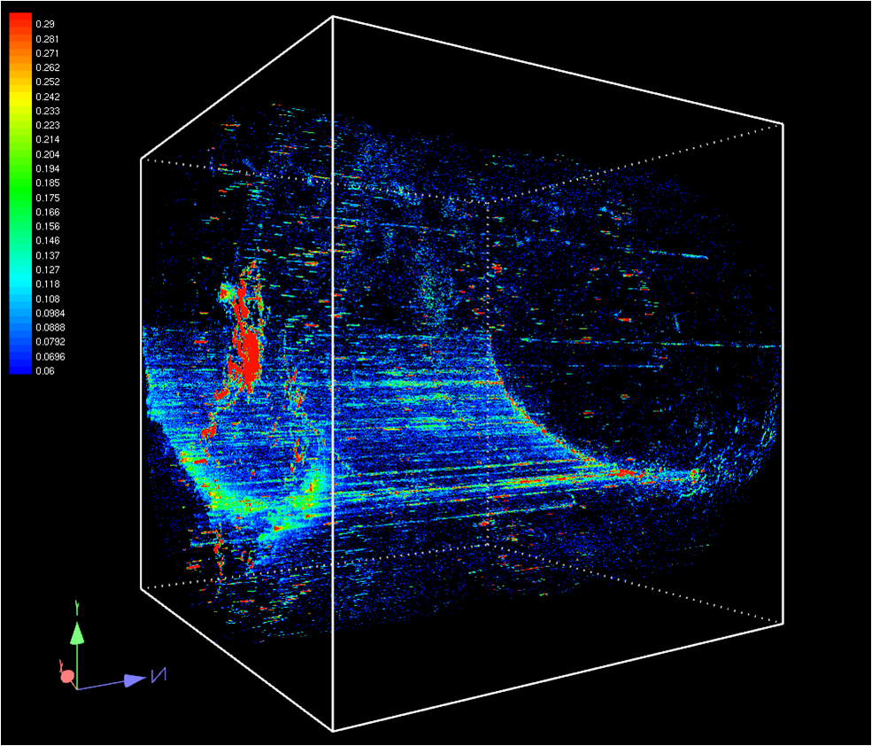
Figure 1: Volume rendering of the HIPASS cube, accomplished with the approach described in this paper. The southern sky cube was generated by Russell Jurek (ATNF) from 387 individual cubes. See Section 1.2 for a description of the features in this cube.

The larger-than-memory problem has been previously examined in astronomy by Beeson et al. (2003) who implemented the distributed shear-warp algorithm (Lacroute and Levoy, 1994) over a Beowulf-style cluster. In their solution (dvr—distributed volume renderer), the volume data was segmented and distributed to cluster nodes, rendered locally, and the (sub-)images were combined by a controlling node using an associative compositing operator. Dvr demonstrated good rendering speeds compared to other solutions at the time, but does not scale well to today’s largest radioastronomy cubes (see their Figure 9). Even if dvr scaled perfectly with no parallelization costs, $\sim 120$ 6-core Westmere processors, with each core handling 20 Mvox sec^-1, would be needed to render the HIPASS cube at 5 fps.

1.3 This work

In this paper, we present a new solution to the larger-than-memory problem, using a significantly smaller computer system than dvr requires for the same input image cube size. Our objective is to provide astronomers with a practical tool to interactively explore and visualize the largest radioastronomy spectral data cubes in real time. Our initial focus is visualizing data from ASKAP, however, it is also applicable to facilities such as LOFAR, ALMA, MWA, and existing large datasets such as the HIPASS cube. We begin with the HIPASS and GASS data cubes as benchmarks to test our solution performance and scalability. Both of these datasets are sufficiently large to provide a valid test of our volume rendering framework (see results section for more details).

This work is about removing a potential technological barrier and enabling astronomers to have a qualitative look at their data as a first step to understanding the complex elements that will occur in the largest radioastronomy datacubes. In particular, we assert that global views can play a vital role as a quality control tool, especially since some of the upcoming facilities (e.g. ASKAP) will not be able to keep all the raw observational data after the initial processing phase. Being able to see the data products from such facilities in a real-time and interactive way may save a lot of precious time and data, and provide opportunities for reprocessing while the raw data products still exist. Furthermore, we anticipate that global views may aid in discovering systematic and non-systematic noise effects, such as signals that vary across the sky due to calibration issues, which may otherwise take huge processing or data reduction effort to determine and extract (e.g. HIPASS data cube in figure 1).

2 Ray casting

A volume rendering is generated by a process called ray casting, which computes the projection of a coloured, semi-transparent volume onto a (finite) 2D viewing plane. The colour and the opacity of each voxel are derived from its data value using a predefined mapping operator called a “transfer function”. For each pixel on the viewing plane, the ray casting process computes a ray originating at this pixel and projects it into the data volume. The ray is traced through the volume, accumulating an aggregate colour and opacity which is assigned to the pixel. The process of compositing any two voxel colours is also defined by the selected transfer function; see Levoy (1990) for a detailed description of the original ray casting algorithm. Although it is a computationally intensive task, ray casting is trivially parallel. This parallel nature has motivated the development of number of parallel ray casting algorithms [e.g. Goel and Mukherjee (1996); Maximo et al. (2008); Scharsach (2005); Jin et al. (2010)].

Graphics Processing Units (GPUs) are the silicon processors used to deliver the computations required for 3D computer graphics. They represent a cheap, commodity hardware (on graphics cards and non-graphics co-processor cards) that can now be utilized as massively-parallel, general purpose computational co-processors, by using software development kits such as CUDA and OpenCL. GPUs have been taken up rapidly by the astronomy computing community [e.g. Hamada et al. (2009); Wayth et al. (2009); Schive et al. (2010)] and in the field of astrophysical visualization, GPUs have been well-utilized for N-body particle data (Kaehler et al., 2006; Li et al., 2008; Szalay et al., 2008; Jin et al., 2010; Becciani et al., 2010). In these examples, GPUs have been used to enhance the rendering speed of the graphics primitives by e.g. $\sim 23$% for the Splotch code (Jin et al., 2010), but these approaches are still limited to datasets that fit within a single machine memory.

Motivated by the appearance of GPUs with large local memory (e.g. 1.7 GB in the AMD ATI Radeon 5970; 1.5 GB in the NVIDIA GX285; up to 4 GB in the NVIDIA Tesla products), and the suitability of the massively-parallel GPU architecture to the ray casting algorithm, we developed a framework which utilizes a heterogeneous CPU and GPU hardware infrastructure, combining shared- and distributed-memory architectures, to yield a scalable volume rendering solution, capable of volume rendering image cubes larger than a single machine memory limit, in real-time and at interactive frame rates. We utilize GPUs as massively-parallel floating point co-processors and consequently, our framework may be suitable for other parallel scientific computing applications, especially those processing or analysing larger-than-memory images.

2.1 Hardware and software architecture

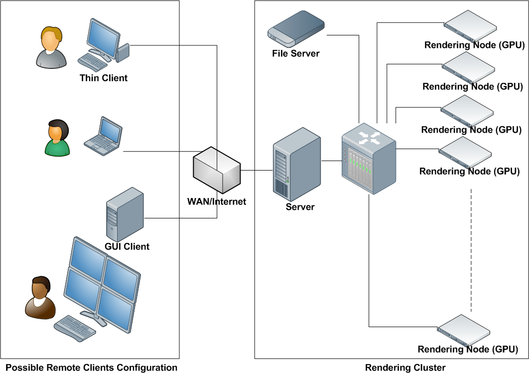
Figure 2: Conceptual diagram for the system hardware architecture. The main system layers are the viewer application, the rendering server, the data/file server, and the rendering client(s). The viewer application may work over different possible remote client’s configuration including Web/Thin client, Desktop machine, or tiled display system.

To address the distributed volume rendering framework, we describe both the hardware and software architecture. Figure 2 shows a conceptual diagram for our hardware architecture. This architecture consists of the following main components:

1. A Cluster of interconnected nodes, each featuring one or more GPU cards and one or more CPU cores;

2. A Server machine, which will schedule tasks, exchange messages between the cluster and the viewer application, for final result composition;

3. Viewer machine(s), which are a regular workstations associated with a display device and I/O mechanism with a connection to the server node; and

4. A File Server, which is a storage node (can be physically any of the processing clients or the server machine) accessible by all the rendering nodes, the server, and the viewer machine.

Based on this architecture configuration, we made the following design assumptions:

• The viewer machine will have only a thin-client application with a small memory and processing requirements. Only a small percentage of the processing will be done on the viewer machine to facilitate the user interactivity, the I/O operations, and the result display. This will make the rendering cluster accessible over geographically distributed locations;

• The final output at arbitrary resolution, can be directed to a single display or a tiled-display system. Although this may decrease the final frame rate, the capability to view a dataset at its full resolution, or even with larger resolution, is very important. For example, some of the small features or details may be hidden if we view ASKAP-size data cubes ($6144\times 6144$ spatial pixels are anticipated) with regular screen resolutions(e.g $1920\times 1200$ for WUXGA is typical); and

• All the rendering nodes and the server can communicate using message passing interface (MPI) . This can be achieved for either a static (the number of cluster nodes is constant) or dynamic cluster (the number of cluster nodes changes with the problem size).

The supporting software architecture utilizes the following software components:

• MPI: for the communication between different rendering nodes and the rendering server;

• NVIDIA Compute Unified Device Architecture (CUDA): for the ray-casting implementation on the GPU;

• Multithreading and message queue: for the communication and management of different GPUs on the same rendering node; and

• TCP direct socket communication: to communicate between the viewer application and the server.

The components described above were integrated in a C++ framework to create a distributed GPU-based rendering farm. This C++ framework orchestrates the process of task distribution, data mapping, compositing, and communication between different GPU kernels, where the actual computation is done. This system assumes that the underlying hardware architecture is heterogeneous, which means that the number of GPUs in each rendering node, the amount of available memory, and possibly even processing power, is different from one node to the next. MPI is used for communication between the different rendering nodes and the rendering server. It has been used because it is the de-facto standard for distributed systems. Only the master thread (i.e. the thread responsible for the local scheduling and communication on each rendering node) on each processing node can communicate directly with the rendering server. Also, the server has no direct control over the processing threads (the threads associate to the GPU units on each node which handle the CUDA kernel invocation and result transfer between GPU memory and the node’s system memory).

The communication between the master thread and the processing threads on each of the rendering nodes is done using a shared Priority Message Queue in a completely asynchronous manner. This method speeds up the communication and minimizes the data sharing between the different threads. Also, it keeps the CUDA function calls within the same thread . When required, any Master thread and the server can communicate together in a synchronous manner. The communication between the server and the viewer application is done through a direct TCP socket. This communication channel is opened and closed via the client and used to transfer control oriented messages and results. The current client implementation uses a QT-based user interface and OpenGL for graphical display and user interaction.

2.2 Rendering overview

The rendering process starts when the user selects a file to render (a menu item on the user interface). The client opens the requested file and loads the associated metadata. The file dimensions, and the recorded minimum and maximum data values are displayed to the user. The user may load the entire cube or a manually specified sub-cube. The user also has the control to use the minimum and the maximum value recorded in the file’s metadata or to ask the server to recalculate the cube minimum and maximum. Next, the file path and the selected cube dimensions are sent to the server to start the data loading process. The server performs a global scheduling task that partitions the cube according to the current rendering nodes. The server then sends a separate file-loading request to each of the processing clients. Each loading request contains the file path and the client’s associated cube portion. In an asynchronous manner, the clients perform a local scheduling task that partitions its associated cube portion, depending on the available GPUs in each client, and start loading data. Once the data is loaded, the data is transferred from the system memory to the GPU memory.

If requested by the user, each GPU calculates the minimum and the maximum of its cube portion, which are then sent back to the server where the global minimum and maximum is calculated. The global minimum and maximum are returned to the client with a data loading confirmation message. The viewer application then generates the color map, which will be used in the rendering, and sends it back to the server as well. After these initialization steps are complete, the server will stay pending for render requests from the viewer application. Whenever the user interacts with the displayed output on the viewer application, the rendering parameters (the transformation and projection matrices) are sent to the server associated with a render request. This render request is distributed over the rendering nodes, which use the GPUs to generate the frame portions and combine (i.e. composite) them. The server performs the final frame composition and sends the result back to the client. The user is also able to perform some other interactions, such as changing the color map, enabling/ disabling spectral channel(s), which are handled in the same manner.

2.3 Data Partitioning

The dataset is partitioned in an object-based manner, which means that each GPU gets only a portion of the data. At the same time each GPU is responsible for generating a portion of the final frame, corresponding to the projection of its assigned data on the current viewing plane using the ray-casting algorithm (Sabella, 1988). The final resultant frame images from each GPU are composited together to produce the final output frame. Figure 3 shows an example data partitioning mechanism. Alternative data partitioning mechanisms could be applied, including more sophisticated techniques like binary space partitioning (Thibault and Naylor, 1987) or an Octree (Samet, 1995).

The data partitioning mechanism affects the final rendering time and the overall performance as we show in Section 3. Based on the data partitioning schema and the viewing angle, the size of the rendering task differs from one GPU to another. Keeping the size of these tasks balanced is an important factor to achieve the highest possible frame rate and interactivity level. We intend to leave further investigation and enhancement to the scheduler as future work. In the current implementation, each scheduling module performs a separate data partitioning decision based on the current longest axis, as shown in Figure 3, so as to achieve a “fair” distribution.

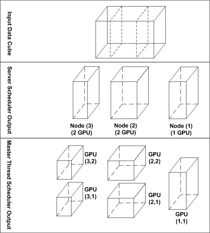
Figure 3: Illustration of the data partitioning process over a cluster configuration of three processing clients. The first and the second processing client have two GPUs, while the third one contains one GPU. The cube partitioning is done based on the longest axis, so in this example the input data cube is partitioned into 3 parts over the X axis. For node 2 and node 3, the longest axis for their assigned cube is the Y axis. Node 1 has only one GPU so no further partition is required.

2.4 Ray-Casting Process

The processing threads are responsible for loading the data portion associated to its assigned GPU and transferring it to the GPU local memory. The GPU memory in our case is the most precious resource, because of the high time cost of data transfer between the GPU memory and the CPU memory, and the limitation of the GPU memory size (will reach 6 GB in the next Fermi GPU , but is limited to 4 GB with the current Tesla cards).

Each processing thread computes a “rendering rectangle”. This rendering rectangle represents the region that the associated GPU is responsible to fill with suitable colors in the final frame. This process is performed using the convex hull algorithm (Graham, 1972); the projection and transformation matrices; and previous knowledge about the extent of the data cube stored in the GPU’s memory. Each ray within the rendering rectangle is tested against the bounding cube for the assigned data portion. In the case where the ray does not intersect with the cube, the current ray sampling process will exit. If the ray intersects with the cube, the entry and exit points are calculated and the sampling distance is determined based on the length of the ray segment, which will be inside the bounding cube. The ray casting kernel employs an early ray-termination mechanism (Levoy, 1990) to speed up the overall rendering process. This mechamism terminates the ray casting process when the accumulated pixel value reach its maximum value. The final output of the ray-casting process is a 2D floating point array of maximum recorded scalar value (in the case of maximum intensity projection) for each pixel.

The usage of these optimization steps minimizes the number of threads needed and the amount of output buffer memory accessed by each GPU, thus speeding up the execution and memory transfer time. We note that these optimization steps do not affect the final output resolution or image quality. Some of these steps are also used to optimize the final frame composition steps, which we now describe.

2.5 Image Composition

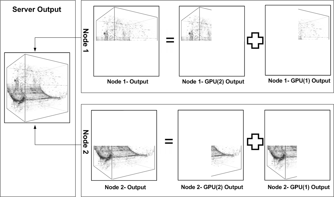
Figure 4: Illustration of the image composition process over a cluster configuration of two processing clients each with two GPUs. A first compositing step occurs on each node, and the final image is combined on the server.

The image composition is performed in two main stages (see Figure 4):

1. Local stage at every rendering node. In this stage, each node is compositing the results generated by its GPUs to generate a single buffer. This composition is done with the guidance of the rendering rectangle for each GPU. Each GPU is executing a composition process only within its rendering rectangle on the final local frame buffer in a sequential manner; and

2. Global stage at the server node. In this stage the server node is compositing the results of all the rendering nodes to generate the final rendering buffer.

The use of this two stage process speeds-up the composition process and minimizes the processing effort required by the server and hence the final rendering time. The final composition complexity and validity depends on the selected transfer function. Lombeyda et al. (2001) provide a mathematical proof that the general alpha-blending volume rendering operator is associative, and can be applied in any blending order.

3 Results

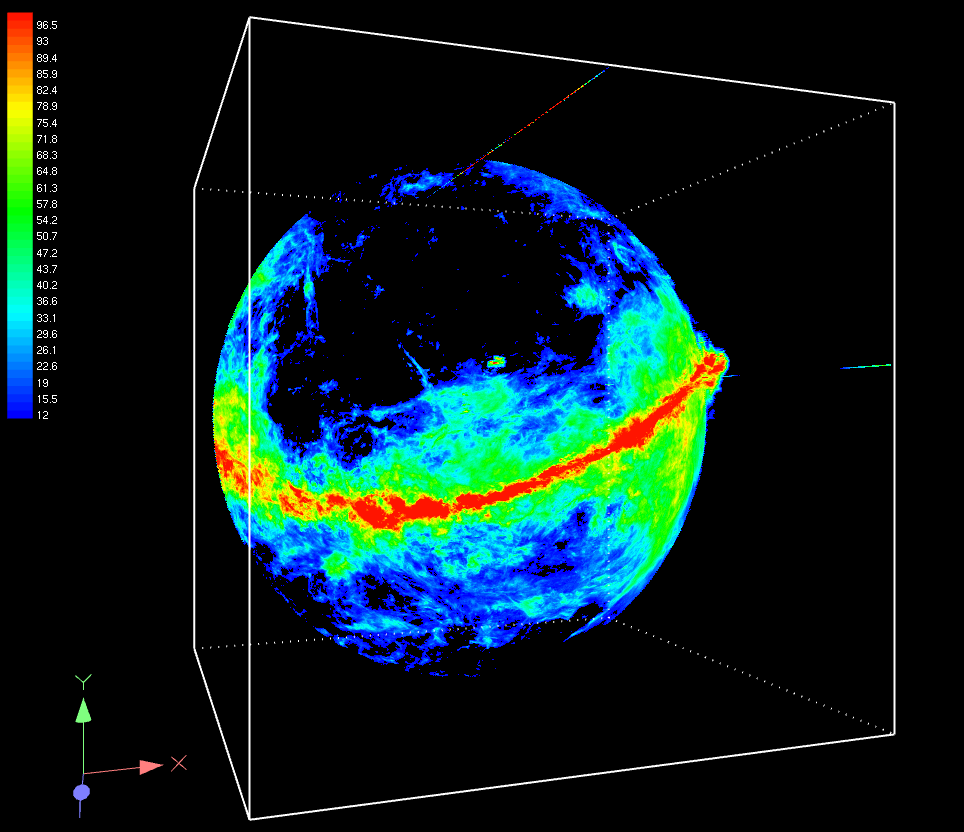
Figure 5: Volume rendering of the GASS cube, accomplished with the approach described in this paper.

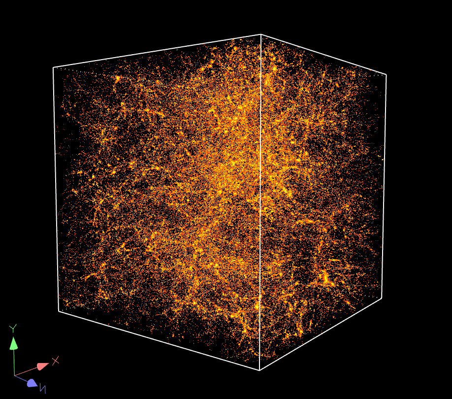
Figure 6: Volume rendering of the Nbody cube, accomplished with the approach described in this paper.

A cluster of four interconnected workstations (the fourth always acting as a server) and nine GPUs (one associated with the server) was used to conduct framework timing tests. The hardware specifications of these workstations are shown in Table 1. Details of the six individual hardware configurations used are shown in Table 2. Tests were performed using a $1024\times 1024$ pixel viewport and a pre-computed sampling distance assuring that each voxel value (intersected by at least one ray) is sampled at least once. The communication is performed over a gigabit Ethernet network. Table 3 shows the details of the datasets used for timing tests. Sample volume rendering are shown for HIPASS cube (Figure 1), GASS cube (Figure 5), and a cube generated from a cosmological N-body simulation (Figure 6, refer Table 3). Although the latter dataset is not from radio astronomy, it demonstrates the applicability of our framework to other 3D data volumes.

We measure the total frame rendering time, $T_{R}$, which is the elapsed time between issuing a rendering request and receiving the rendered frame back. $T_{R}$ is an indication of the number of frames per second that the framework can render, and is a summation of the time spent on different framework sub-processes.

$$T_{R}=\rm{Max}(T_{\rm{ray}(i)})+\rm{Max}(T_{\rm{merge}(j)})+{}$$ (1)

$${}+\rm{Max}(T_{\rm{comm}(j)})+T_{\rm{server}}\pm\epsilon$$

Where $1\leq i\leq\mbox{Number of GPUs}$, $1\leq j\leq\mbox{Number of Workstations}$, $T_{\rm{ray}}$ indicates the time spent on the GPU doing ray tracing, $T_{\rm{merge}}$ is the time spent on each client for local merging, $T_{\rm{comm}}$ is the communication time between each workstation and the server, and $T_{\rm{server}}$ is the time spent by the server doing the global merging. The last component, $\epsilon$, indicates that variation happens due to the overlapping effect and any unexpected delays (see below).

Due to the framework’s distributed behaviour and the heterogeneous hardware, the maximum time spent in each sub-process is dominated by the time spent by the slowest processing element. For example, the ray casting process times vary between different GPUs based on the cube’s orientation, which effects the size of the rendering rectangle of the dataset portion. This affects the number of rays that need to be traced and the path-length of the rays through the volume, which in turn affects the number of sampling operations required for each ray. Overlaps between communication and computation usually eliminate the differences between processing elements, but due to the randomness of this overlapping order, its effect is not constant.

Figure 7 shows a sample timing diagram for the HIPASS cube as a function of cube orientation, using the 2P4G configuration (see Table 2). The rendering time depends on the cube orientation, which is represented by the rotation angle, $\theta$, about the y-axis in degrees. $T_{ray}$ is the dominating factor for the variation in the rendering time with an average near 50%. Also, a small variation between the frame rendering times for opposite angles, ($\theta$ and $180^{\circ}+\theta$), is caused by the early ray termination optimization step in the ray tracing implementation. The value of $\rm{Max}(\rm{T}_{\rm{merge}})$ , $\rm{Max}(\rm{T}_{\rm{comm}})$, and $\rm{Max}(\rm{T}_{\rm{server}})$ are almost constant, because they are directly proportional to the final frame output size, which is not affected by the cube orientation.

Figure 8 shows the average, minimum, and maximum frame rendering time for the HIPASS cube for different cluster configurations. Figure 9 shows the average, minimum, and maximum frame rendering time for the three datasets using the 3P8G configuration. Based on these timing tests, we can conclude that:

1. Increasing the number of GPUs does not necessarily reduce the final rendering time. Due to the communication and compositing overheads, for a fixed number of GPUs, the lower the number of workstations, the lower the frame rendering time.

2. The unbalanced distribution of rendering tasks over the GPUs limits the framework speedup. Although different rendering tasks are being performed in parallel, the total frame rendering time is dominated by the maximum GPU rendering time as shown in equation 1. The current scheduler implementation uses the dataset dimensions and the GPU computational power (number of cores and memory size) to fairly partition the dataset over the rendering nodes and GPUs. But the problem size each GPU tries to solve varies based on the dataset characteristics (affects early ray termination), and the traced rays’ length (because of perspective projection). Figures 10 and 11 demonstrate this by showing the different sub-frame rendering time for each GPU for the HIPASS cube using the 2P4G configuration. Based on the variation in the difference between the maximum, the average, and the minimum rendering time, we expect this “unbalanced distribution” influence to disappear with a large increase in the number of GPUs. On the other hand, the average total frame rendering time without early ray termination and with orthographic projection is higher by 12 % from the average total frame rendering time with the early ray termination and perspective projection. The usage of a better data partitioning and scheduling which depends on the dataset characteristics and dimensions may also improve this behaviour.

Figure 12 shows timing for the HIPASS data cube with two different output sizes $1024\times 1024$ and $512\times 512$ pixels. The timing follows the same pattern for both output sizes but with an average time reduction of 69%. This reduction in the frame rendering time is due to the reduction in $T_{ray}$, the reduction in the size of merging operations, and the size of the data exchanged between the rendering workstations and the server.

Table 1: Hardware specification for the cluster used to evaluate the performance of our framework.

Index	GPU Model	GPU memory	Processor Model	System memory
1	4x NVIDIA Tesla C1060	4 Gigabyte/GPU	16x Intel Xeon X5550	18 Gigabyte
2	2x NVIDIA Tesla C1060	4 Gigabyte/GPU	2x Nehalem i7	24 Gigabyte
3	4x NVIDIA Tesla C1060	4 Gigabyte/GPU	2x Nehalem i7	24 Gigabyte
4	1x GeForce GTX 285	1 Gigabyte	1x Intel i7 930	12 Gigabyte

Table 2: Details of the hardware configurations of the cluster (GPU+CPU) used to evaluate performance. The letter ‘P’ is used as an abbreviation for the number of processing workstation, and the letter ‘G’ is used as an abbreviation for the number of GPUs. The configurations do not include the server.

Configuration	Client(1)	Client(2)	Client(3)	Server
1 P 4 G	4			1
2 P 4 G	2	2		1
3 P 5 G	2	2	1	1
3 P 6 G	2	2	2	1
3 P 7 G	2	2	3	1
3 P 8 G	2	2	4	1

Table 3: Sample datasets used to evalute the performance of our framework.

Dataset Name	Dimensions (Data Points)	Source / Credits	File Size
Nbody cube	1024 x 1024 x 1024	High resolution $1080^{3}$ dark matter simulation of a 125 Mpc/h box by Swinburne Computations for WiggleZ (SCWiggleZ) project (Poole et al 2010, in prep)	4 Gigabyte
HIPASS Cube	1721 x 1721 x 1025	HIPASS Southern Sky, data courtesy Russell Jurek/HIPASS team	12 Gigabyte
GASS Cube	2502 x 2501 x 1093	The Parkes Galactic All-Sky Survey, data courtesy Naomi McClure-Griffiths/ GASS team (McClure-Griffiths et al., 2009)	26 Gigabyte

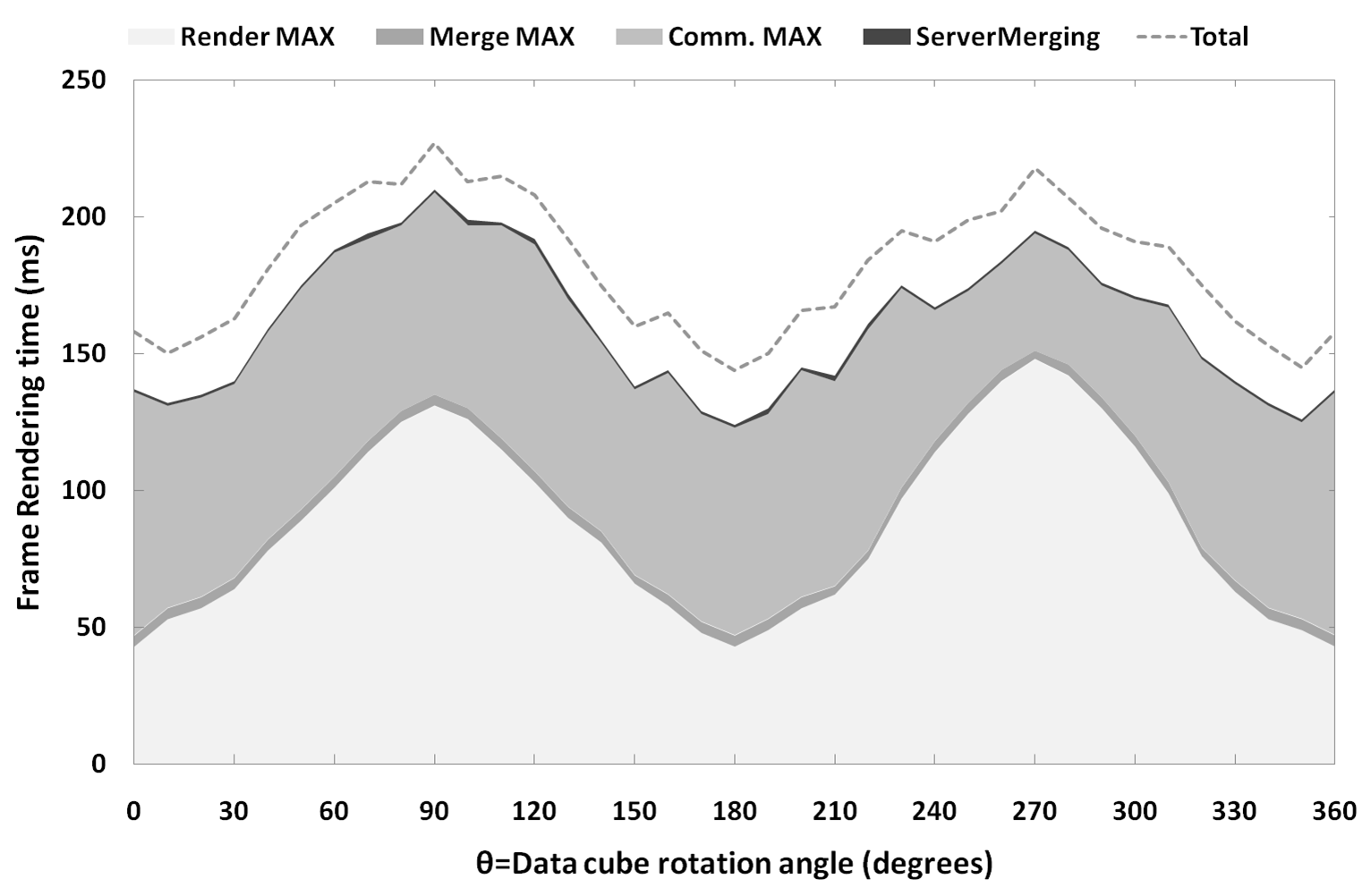
Figure 7: Single frame rendering times for different cube rotation angles. The timing measurements were done for the HIPASS Southern Sky data cube on 3 workstations (one acting as a server) and 4 GPUs (2 P 4 G).

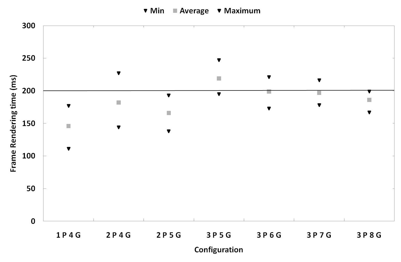
Figure 8: Minimum, average, and maximum rendering time for the HIPASS data cube using different hardware configurations. The horizontal line shows our target of 5 fps for real-time interaction.

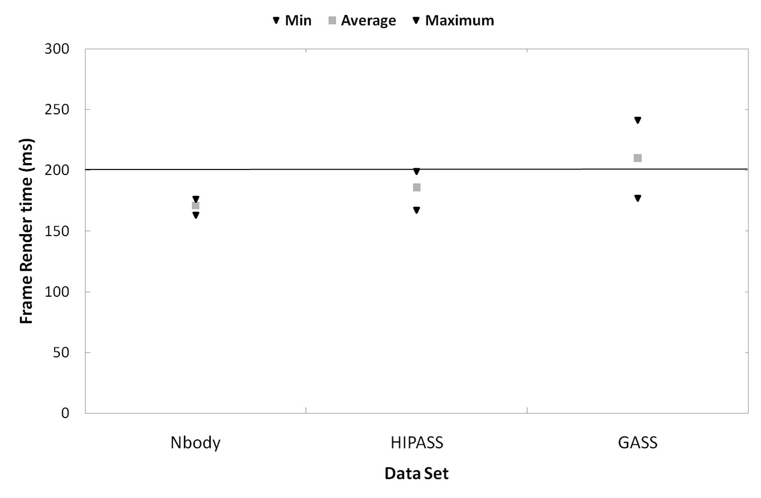
Figure 9: Minimum, average, and maximum rendering time for the HIPASS cube, GASS Cube, and Nbody cube using the 3P8G configuration.

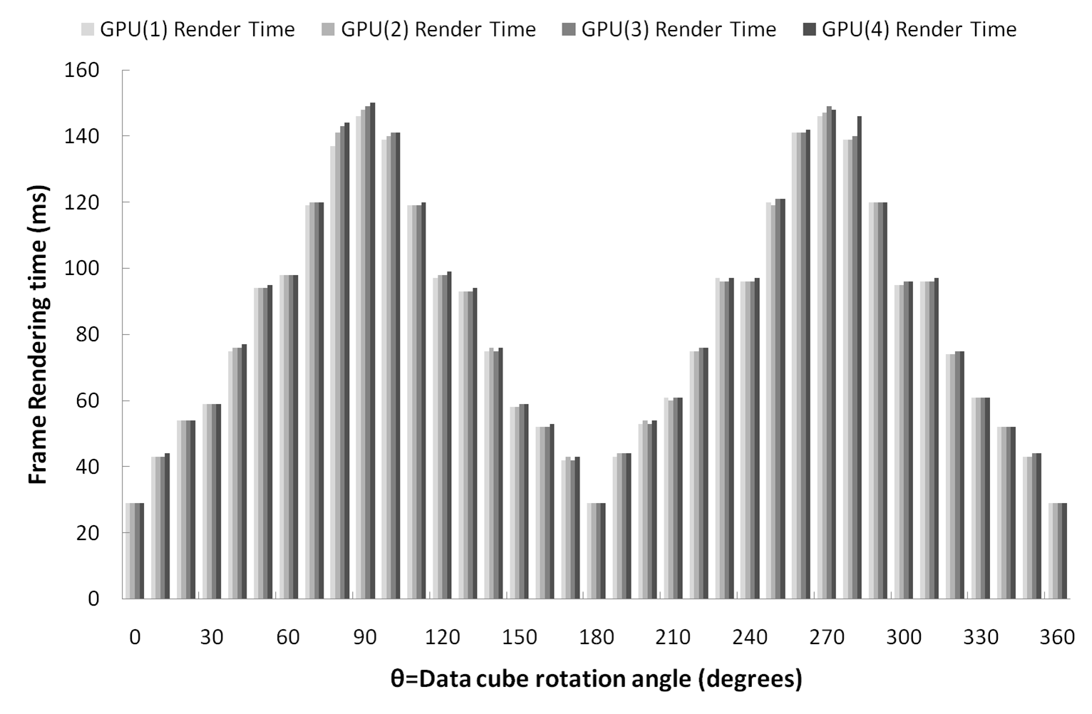
Figure 10: Different GPU sub-frame rendering time for the HIPASS cube using the 2P2G configuration with early ray termination deactivated and orthographic projection.

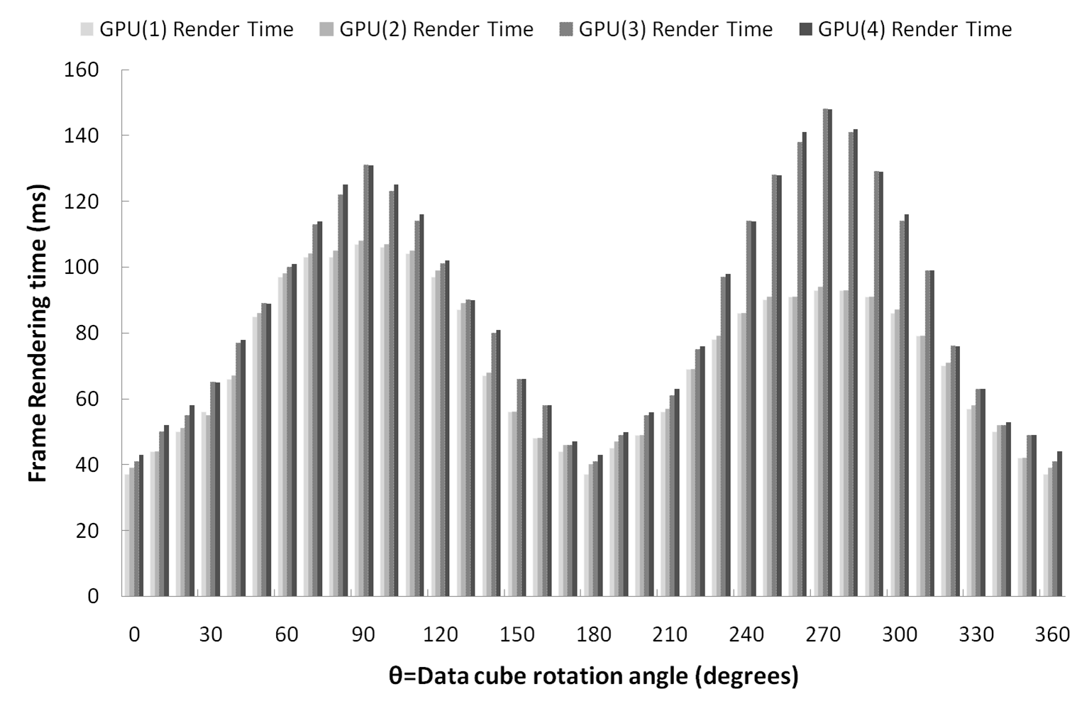
Figure 11: Different GPU sub-frame rendering time for the HIPASS cube using the 2P2G configuration with early ray termination enabled and perspective projection.

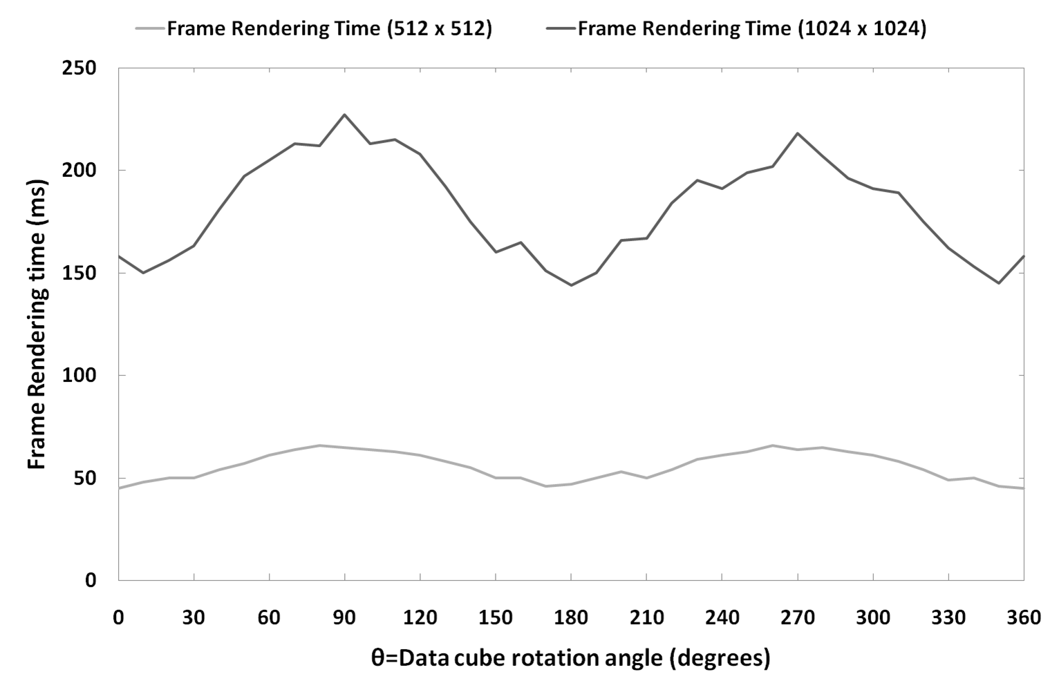
Figure 12: Single frame rendering times for different cube rotation angles with different output sizes ( $1024\times 1024$ and $512\times 512$ pixels). The timing measurement was done for the HIPASS cube on 3 workstations (one acting as a server) and 4 GPUs (2 P 4 G).

4 Discussion

4.1 Framework performance and scalability

In order to evaluate the performance gain from adopting GPUs as the main processing elements, we compared our performance timing with the distributed volume rendering implementation (dvr) introduced by Beeson et al. (2003). The main performance evaluation done for dvr used 2 GHz Pentium 4 CPUs and was able to render around 7 MVox/s. If we scale that to current CPU clock speeds (e.g. Westmere 2.93GHz processor), dvr should be capable to render 120 MVox/s with 6 cores. Consequently, using equation (7) of Beeson et al. (2003) and by assuming perfect scalability, dvr needs approximetely 120 $\times$ 6-core Westmere processors in order to render the HIPASS cube with 5 fps, while our framework can render that cube with 4 GPUs.

During our performance and timing tests, we were unable to obtain a data file larger than the GASS data cube (26 GB). Furthermore, access to a larger GPU cluster was not available. Although we remain cautious about conclusions related to scalability of our framework, we believe it should be able to handle larger datasets, even of Terabyte order, if proper hardware infrastructure is available. We base this conclusion on the following:

• the amount of data transfer between the rendering workstation and the server is almost constant and depends on the output resolution rather than the input data size;

• the usage of ray casting combined with the rendering rectangle optimization makes the problem size almost constant for the rendering and the communication between the nodes;

• the overlapping between the computation and communication minimizes the communication delay;

• the two stage frame composition minimizes the amount of the processing required by the server and the amount of data exchanged between the clients and the server; and

• the local and global composition processes are done on GPU with a negligible cost compared to the rendering time.

Moreover, the on-going increase in number of processing cores and size of local memory of GPUs will help to decrease the rendering time and minimize the number of GPUs needed to render a certain data size. For example the next generation of NVIDIA Tesla GPUs is expected to have double the current number of processing elements and 1.5 times the current memory size.

4.2 Future Work

We expect the performance of our framework will be dramatically enhanced by using the next NVIDIA GPU architecture, code-named Fermi. Features like predicated instructions, larger local memory, larger memory address space, greater DRAM bandwidth, improved instruction scheduler, and higher FLOP/S will provide our system with more powerful hardware infrastructure and remove some of the software bottlenecks. Also, utilizing the direct integration between the Tesla cards and an InfiniBand network infrastructure may decrease the communication overhead and provide improved scalability.

To overcome the current GPU memory size limitation, we believe that lossy compression of the cube portions stored in the GPU local memory, using wavelet compression, will enable us to store and render larger cubes without affecting the final render quality. There have been a few trials to visualize datasets stored in the compressed wavelet format (Nguyen and Saupe, 2001; Guthe et al., 2002), but to our knowledge none of these algorithms have been ported to GPU yet. It is likely that wavelet techniques can also be applied as a noise removal tool to increase the output quality. The usage of wavelet compression was demonstrated by Pence et al. (2009) with optical data, however, some modifications are required to enable fast decompression and retrieval of random data positions (Nguyen and Saupe, 2001).

Quantitative data visualization support is still a missing ingredient from a complete visualization and analysis system for astronomy, and may be the main factor limiting a wider adoption of 3D visualization in astronomy. We aim to examine this further in future work. A closely related issue is the use of noise-suppression techniques, as faint signals may be hidden in large-scale noise features. Designing one or more specialized transfer functions can provide the user with better visualization results. Most of the current well known transfer functions may not provide the user with the best visualization output because they were designed to serve other scientific domains. Transfer functions capable of suppressing noise and emphasising important data features will provide the users with better visualization outcomes and enhance the usefulness of 3D visualization as a data analysis and knowledge discovery tool.

5 Conclusion

Visualization is a valuable tool for knowledge discovery. Along with providing insight and opportunities for analysis of sources under investigation, global views of data are vital for the detection of instrumentation errors, and the identification of data artefacts and noise characteristics. New approaches are needed to visualize the massive, Terabyte order, data cubes that will be produced routinely by facilities such as ASKAP, MeerKat, LOFAR and ultimately, the Square Kilometre Array.

In this work, we have introduced a framework to visualize larger than memory multispectral 3D datasets. The framework provides the user with a real-time interactive volume rendering by combining between shared and distributed memory architectures, employing a distributed GPU infrastructure, and using the ray-casting volume rendering algorithm. We are trying to provide astronomers with a more affordable solution to deal with the upcoming data avalanche, by offering GPUs as an alternative to the currently used distributed computing infrastructures. By reducing the number of machines required to handle such datasets we not only reduce the overall hardware cost but also we provide an easier to deploy, and hence manage, solution. A remote viewer application is used to enable the user to control and interact with the framework. System implementation was done using QT, MPI, and CUDA within a C++ object oriented framework.

Framework performance was evaluated using a cluster of four workstations and nine GPUs. The performance evaluation and timing tests were used to show the framework scalability, how different framework processes contribute to the final rendering time, and the effect of changing the cube orientation and the output viewport size on the rendering time. Medium size (12 GB) and relatively larger data cube (26 GB) were used throughout the timing tests. The maximum total rendering time for a 26 GB data cube with a $1024\times 1024$ output viewport was $<0.3$ second, with frame rates of 5 fps achievable.

Based on the framework performance and timing analyses, we believe it should be able to visualize larger datasets, even of Terabyte order, if proper hardware infrastructure is available. The usage of ray casting, the overlapping between communication and computation, and the two stage results compositing minimize the parallelization overhead and the final frame rendering time.

References

References

- Barnes et al. (2001) Barnes, D. G., Staveley-Smith, L., de Blok, W. J. G., Oosterloo, T., Stewart, I. M., Wright, A. E., Banks, G. D., Bhathal, R., Boyce, P. J., Calabretta, M. R., Disney, M. J., Drinkwater, M. J., Ekers, R. D., Freeman, K. C., Gibson, B. K., Green, A. J., Haynes, R. F., te Lintel Hekkert, P., Henning, P. A., Jerjen, H., Juraszek, S., Kesteven, M. J., Kilborn, V. A., Knezek, P. M., Koribalski, B., Kraan-Korteweg, R. C., Malin, D. F., Marquarding, M., Minchin, R. F., Mould, J. R., Price, R. M., Putman, M. E., Ryder, S. D., Sadler, E. M., Schröder, A., Stootman, F., Webster, R. L., Wilson, W. E., Ye, T., 2001. The Hi Parkes All Sky Survey: southern observations, calibration and robust imaging. mnras 322, 486–498.
- Becciani et al. (2010) Becciani, U., Costa, A., Antonuccio-Delogu, V., Caniglia, G., Comparato, M., Gheller, C., Jin, Z., Krokos, M., Massimino, P., 2010. VisIVO–Integrated Tools and Services for Large-Scale Astrophysical Visualization. PASP 122, 119–130.
- Beeson et al. (2003) Beeson, B., Barnes, D., Bourke, P., 2003. A distributed-data implementation of the perspective shear-warp volume rendering algorithm for visualisation of large astronomical cubes. PASA 20, 300–313.
- Beeson et al. (2004) Beeson, B., Lancaster, M., Barnes, D., Bourke, P., Rixon, G., 2004. Visualizing astronomy data using VRML. In: Proceedings of SPIE. Vol. 5493. pp. 242–253.
- Brugel (1993) Brugel, E., 1993. Visualization techniques to aid in the analysis of multi-spectral astrophysical datasets. Tech. rep., University of Colorado, Department of Computer Science, Boulder.
- Domik and Mickus-Miceli (1992) Domik, G., Mickus-Miceli, K., 1992. Software Design and Development In a Scientific Environment: Lessons Learned During the Development of STAR, an Astrophysical Analysis and Visualization Package. In: Astronomical Data Analysis Software and Systems I. Vol. 25. p. 95.
- Drebin et al. (1988) Drebin, R., Carpenter, L., Hanrahan, P., 1988. Volume rendering. ACM Siggraph Computer Graphics 22 (4), 74.
- Fluke et al. (2010) Fluke, C., English, J., Barnes, D., 2010. Visualization-Directed Interactive Model-Fitting to Spectral Data Cubes. Arxiv preprint arXiv:1001.2043.
- Goel and Mukherjee (1996) Goel, V., Mukherjee, A., 1996. An optimal parallel algorithm for volume ray casting. The Visual Computer 12 (1), 26–39.
- Gooch (1995) Gooch, R., 1995. Astronomers and their shady algorithms. In: IEEE Conference on Visualization, 1995. Visualization’95. Proceedings. pp. 374–377.
- Graham (1972) Graham, R., 1972. An efficient algorith for determining the convex hull of a finite planar set. Information Processing Letters 1 (4), 132–133.
- Guthe et al. (2002) Guthe, S., Wand, M., Gonser, J., Strasser, W., 2002. Interactive rendering of large volume data sets. IEEE Visualization, 2002. VIS 2002, 53–60.
- Hamada et al. (2009) Hamada, T., Narumi, T., Yokota, R., Yasuoka, K., Nitadori, K., Taiji, M., 2009. 42 tflops hierarchical n-body simulations on gpus with applications in both astrophysics and turbulence. In: SC ’09: Proceedings of the Conference on High Performance Computing Networking, Storage and Analysis. ACM, New York, NY, USA, pp. 1–12.
- Jin et al. (2010) Jin, Z., Krokos, M., Rivi, M., Gheller, C., Dolag, K., Reinecke, M., april 2010. High-performance astrophysical visualization using Splotch. ArXiv e-prints.
- Kaehler et al. (2006) Kaehler, R., Wise, J., Abel, T., Hege, H., 2006. GPU-assisted raycasting for cosmological adaptive mesh refinement simulations. In: Eurographics/IEEE VGTC Workshop on Volume Graphics (Boston, Massachusetts, USA, 2006), Eurographics Association. Citeseer, pp. 103–110.
- Lacroute and Levoy (1994) Lacroute, P., Levoy, M., 1994. Fast volume rendering using a shear-warp factorization of the viewing transformation. In: Proceedings of the 21st annual conference on Computer graphics and interactive techniques. ACM, p. 458.
- Levoy (1990) Levoy, M., 1990. Efficient ray tracing of volume data. ACM Transactions on Graphics (TOG) 9 (3), 261.
- Li et al. (2008) Li, H., Fu, C., Hanson, A., 2008. Visualizing Multiwavelength Astrophysical Data. IEEE Transactions on Visualization and Computer Graphics 14 (6), 1555–1562.
- Lombeyda et al. (2001) Lombeyda, S., Moll, L., Shand, M., Breen, D., Heirich, A., 2001. Scalable interactive volume rendering using off-the-shelf components. In: PVG ’01: Proceedings of the IEEE 2001 symposium on parallel and large-data visualization and graphics. IEEE Press, Piscataway, NJ, USA, pp. 115–121.
- Magnor et al. (2005) Magnor, M., Hildebrand, K., Lintu, A., Hanson, A., 2005. Reflection nebula visualization. IEEE Visualization, 2005. VIS 05, 255–262.
- Maximo et al. (2008) Maximo, A., Ribeiro, S., Bentes, C., Oliveira, A., Farias, R., 2008. Memory efficient gpu-based ray casting for unstructured volume rendering. In: IEEE/EG Int. Symp. Volume and Point-Based Graph. pp. 55–62.
- McClure-Griffiths et al. (2009) McClure-Griffiths, N. M., Pisano, D. J., Calabretta, M. R., Ford, H. A., Lockman, F. J., Staveley-Smith, L., Kalberla, P. M. W., Bailin, J., Dedes, L., Janowiecki, S., Gibson, B. K., Murphy, T., Nakanishi, H., Newton-McGee, K., Apr. 2009. Gass: The Parkes Galactic All-Sky Survey. I. Survey Description, Goals, and Initial Data Release. ApJS 181, 398–412.
- Nadeau et al. (2001) Nadeau, D., Genetti, J., Napear, S., Pailthorpe, B., Emmart, C., Wesselak, E., Davidson, D., 2001. Visualizing stars and emission nebulae. In: Computer Graphics Forum. Vol. 20. pp. 27–33.
- Nguyen and Saupe (2001) Nguyen, K., Saupe, D., 2001. Rapid high quality compression of volume data for visualization. In: Computer Graphics Forum. Vol. 20. pp. 49–57.
- Norris (1994) Norris, R., 1994. The Challenge of Astronomical Visualisation. In: Astronomical Data Analysis Software and Systems III. Vol. 61. p. 51.
- Oosterloo (1995) Oosterloo, T., 1995. Visualisation of Radio Data. In: Astronomical socity of Australia Proceedings. Vol. 12. p. 215.
- Oosterloo (1996) Oosterloo, T., 1996. Adaptive filtering and masking of HI data cubes. VA 40 (4), 571–577.
- Pence et al. (2009) Pence, W., Seaman, R., White, R., 2009. Lossless astronomical image compression and the effects of noise. PASP 121, 000–000.
- Sabella (1988) Sabella, P., 1988. A rendering algorithm for visualizing 3D scalar fields. In: Proceedings of the 15th annual conference on Computer graphics and interactive techniques. ACM, p. 58.
- Samet (1995) Samet, H., 1995. Spatial data structures. Modern Database Systems: The Object Model, Interoperability and Beyond, 361–385.
- Scharsach (2005) Scharsach, H., 2005. Advanced GPU raycasting. Proceedings of CESCG 5, 67–76.
- Schive et al. (2010) Schive, H., Tsai, Y., Chiueh, T., 2010. GAMER: A Graphic Processing Unit Accelerated Adaptive-Mesh-Refinement Code for Astrophysics. ApJS 186, 457–484.
- Schwarz (2007) Schwarz, N., 2007. Distributed Volume Rendering of Very Large Data on High-Resolution Scalable Displays. Master’s thesis, University of Illinois, Chicago.
- Szalay et al. (2008) Szalay, T., Springel, V., Lemson, G., Nov. 2008. GPU-Based Interactive Visualization of Billion Point Cosmological Simulations. ArXiv e-prints.
- Thibault and Naylor (1987) Thibault, W., Naylor, B., 1987. Set operations on polyhedra using binary space partitioning trees. ACM SIGGRAPH Computer Graphics 21 (4), 162.
- Wayth et al. (2009) Wayth, R. B., Greenhill, L. J., Briggs, F. H., 2009. A gpu-based real-time software correlation system for the murchison widefield array prototype. PASP 121 (882), 857–865.