Asymptotic solution for first and second order integro-differential equations

Abstract

This paper addresses the problem of finding an asymptotic solution for first and second order integro-differential equations containing an arbitrary kernel, by evaluating the corresponding inverse Laplace and Fourier transforms. The aim of the paper is to go beyond the tauberian theorem in the case of integral-differential equations which are widely used by the scientific community. The results are applied to the convolute form of the Lindblad equation setting generic conditions on the kernel in such a way as to generate a positive definite density matrix, and show that the structure of the eigenvalues of the correspondent liouvillian operator plays a crucial role in determining the positivity of the density matrix.

1 Introduction

The Laplace and Fourier transforms are powerful tools widely used in scientific fields such as mathematics, physics, biology and chemistry. These transforms are often applied to linear partial differential equations and integro-differential equations to eliminate time and space dependence. The analytical solutions thus obtained need to be inverted to the time and space domain (see [1] for a monograph on the Laplace transform). Santos [2] found a procedure for an analytical inversion of the Laplace transform reducing the inversion formula to an integration on the interval $[0,\infty)$. While literature on the numerical inversion of the Laplace transform is rich (see [3] for a review) the analytical inversion still rests mostly on the tauberian theorem. This paper focuses on first and second order integro-differential equations containing an arbitrary kernel. It is virtually impossible to list a complete bibliography on the topic and for this reason the reader is referred to the following exemplary papers [4, 5, 6, 7, 8]. In these works the authors discuss the first order integro-differential equation of the form

$$\frac{d}{dt}F(t)-zF(t)=\int_{0}^{t}K(t-t^{\prime})F(t^{\prime})dt^{\prime}$$ (1)

or, after applying the Laplace transform, the equivalent equation

$$\hat{F}(u)=\frac{F(0)}{u-z-\hat{K}(u)}$$ (2)

where, by definition $\hat{F}(u)=\int_{0}^{\infty}\exp[-ut]F(t)dt$. The above equation, Eq. (2), represents a typical form that leads the process for finding a solution of the original problem stated by Eq. (1). Once the transformed function is obtained the inversion process is often a difficult task. In this paper we shall consider the inversion of a Laplace transform of the form

$$\hat{F}(u)=\frac{1}{P_{n}(u)+\varepsilon\hat{K}(u)}$$ (3)

and analogously, of a Fourier transform of the form

$$\hat{F}(\omega)=\frac{1}{P_{n}(\omega)+\varepsilon\hat{K}(\omega)}$$ (4)

where $P_{n}(u)$ or $P_{n}(\omega)$ is a $n$-degree polynomial, $\varepsilon$ is a parameter, and $\hat{K}(u)$ or $\hat{K}(\omega)$ is an arbitrary function. Without loss of generality we shall consider the case of the Laplace transform. With slight changes, the results may be applied to the Fourier transform.

The main goal of this paper is to give a prescription to find an asymptotic expression for the function $F(t)$ in the representation of the starting variable, typically the time domain for the Laplace transform, or the space domain for the Fourier transform. This problem is partially solved by the use of the tauberian theorem but, as it is well known, the conditions for correctly applying this theorem are quite strict. We shall focus on the case of $P_{1}(u)=u+a$ and $P_{2}(u)=u^{2}\pm a^{2}$ giving sufficient conditions on $\hat{K}(u)$ that allow us to find an approximate expression for either the inverse Fourier or the Laplace transforms.

This work is organized as follows: In Sec. 2 we consider a short review for the case when the function $\hat{K}(u)$ is a generic polynomial such that an analytical expression for the asymptotic solution $F(t)$ is given when $P_{n}(u)$ is both a first and second degree polynomial. In Sec. 3 we adopt the multi-scale approach to find an approximate solution for the case when $P_{n}(u)$ is a second degree polynomial and $\hat{K}(u)$ is a generic function. In Sec. 4 the problem is solved in a less generic way but it is mathematically rigorous. An equation for the asymptotic expression of $F(t)$ generated by Eq. (1) shall be found. Such an equation is independent of the form of the kernel. This is why we can use the term universality to describe the asymptotic equation. Finally, in Sec 5 the previous results are applied to the case of the convoluted Lindblad equation [9, 10] whereby we discuss the sufficient conditions on the kernel to obtain a positive definite quantum density matrix.

2 Laplace transform containing polynomials

In this section we briefly examine the polynomial case, however before exposing the main idea let us clarify a key point. Intuitively, we could say that for $\varepsilon\to 0$ the inverse Laplace transform of Eq. (3) can be evaluated at the poles of the unperturbed polynomial. Moreover, we could try to apply the tauberian theorem to ”guess” the asymptotic solution. The following example shows that, in general, the problem can be much more complex. To illustrate the main idea let us consider the following Laplace transform

$$\hat{F}(u)=\frac{1}{u+1+\varepsilon\left(u^{3}+u^{2}\right)}.$$ (5)

Naively we could say that for $\varepsilon\to 0$, then $F(t)\approx\exp[-t]$. First, let us find the solution neglecting $u^{3}$ employing the tauberian theorem idea. The poles can be evaluated analytically and its expressions are

$$u_{1}=\frac{-1-\sqrt{1-4\varepsilon}}{2\varepsilon},\,\,\,\,u_{2}=\frac{-1+\sqrt{1-4\varepsilon}}{2\varepsilon}.~{}$$

Consequently the solution is

$$F(t)=\frac{2e^{-\frac{t}{2\varepsilon}}\sinh\left[\frac{t\sqrt{1-4\varepsilon}}{2\varepsilon}\right]}{\sqrt{1-4\varepsilon}}\approx-\exp\left[\frac{-t}{\varepsilon}+t\right]+\exp[-(1+\varepsilon)t]\approx\exp[-t]$$ (6)

which seems to support the idea that for $\varepsilon\to 0$, then $F(t)\approx\exp[-t]$. If we evaluate the exact poles

$$u_{1}=-1,\,\,\,\,u_{2}-\frac{\imath}{\sqrt{\varepsilon}},\,\,\,\,u_{3}=\frac{\imath}{\sqrt{\varepsilon}},$$

the exact solution is

$$F(t)=\frac{e^{-t}}{1+\varepsilon}+\frac{-\cos\left[\frac{t}{\sqrt{\varepsilon}}\right]+\sqrt{\varepsilon}\sin\left[\frac{t}{\sqrt{\varepsilon}}\right]}{1+\varepsilon}.$$ (7)

Note that the limit for $\varepsilon\to 0$ of solution (7) does not exist. The previous example clarifies an important point. In general, for $\varepsilon\to 0$, it is not correct to invert the Laplace transform evaluating the approximate poles of the unperturbed polynomial [see Eq. (6)]. The reason why the expansion in power of the variable $u$ fails in the polynomial case is because by neglecting higher powers we are neglecting poles that are divergent for $\varepsilon\to 0$.

We now consider a second degree polynomial for $P_{n}(u)$, namely $P_{2}(u)$, and at the end of this section we shall consider a first degree polynomial, $P_{1}(u)$. Without loss of generality, we shall focus on the case $P_{2}(u)=u^{2}\pm a^{2}$. We start by considering $\hat{K}(u)=G_{n}(u)$ where $G_{n}(u)=\sum_{k=0}^{n}a_{k}u^{k}$ is a polynomial of $n$ degree with $n>2$. If we want an approximate solution of $\varepsilon$ order we must evaluate all the poles in addition to the two given by

$$\bar{u}_{1,2}=\pm\sqrt{-a^{2}-\varepsilon G_{n}(\sqrt{-a^{2}})}.$$

To fix the ideas, we select $P_{2}(u)=u^{2}+a^{2}$. Looking for a scaling such that the term $u^{n}$ is of the same order of $u^{2}$, we perform the transformation $u\to\varepsilon^{\nu}U~{}$ so that we have

$$\varepsilon^{2\nu}=\varepsilon^{n\nu+1}.$$ (8)

Equating the exponents we find that $\nu=-\frac{1}{n-2}$. Keeping only the lowest order, we obtain the poles for the polynomial equation

$$a_{n}U^{n}_{0}+U^{2}_{0}=0.$$ (9)

The solution can be easily found as

$$U_{0}(k)=\frac{1}{\mid a_{n}\mid^{\frac{1}{n-2}}}\exp\left[\frac{\imath\phi}{n-2}+\frac{2k\pi\imath}{n-2}\right],\,\,\,\,\,k=0,\cdots n-3$$ (10)

with $\phi=\arg(-a_{n})$. Eq. (10) gives $n-2$ solutions that, combined with the two solutions given by

$$\bar{u}_{1,2}=\pm\sqrt{-a^{2}-\varepsilon G_{n}(\sqrt{-a^{2}})},$$

complete the $n$ solutions for the total polynomial. The next order for the $n-2$ divergent solutions is given by:

$$U_{1}(k)=-\frac{a_{n-1}}{(n-2)a_{n}}.$$ (11)

Using the residue theorem we find the inverse Laplace transform by evaluating the integral

$$F(t)=\frac{1}{2\pi\imath}\int\limits_{-\imath\infty+\gamma}^{\imath\infty+\gamma}\frac{\exp[ut]}{P_{2}(u)+\varepsilon G_{n}(u)}du$$ (12)

at the poles given by

$$u_{k}=\frac{U_{0}(k)}{\varepsilon^{\frac{1}{n-2}}}-\frac{a_{n-1}}{(n-2)a_{n}},\,\,k=0\cdots n-3,\,\,\bar{u}_{1,2}=\pm\sqrt{-a^{2}-\varepsilon G_{n}(\sqrt{-a^{2}})}.$$ (13)

The approximate expression for the function $F(t)$ is

$$F(t)=\frac{\exp[\bar{u}_{1}t]}{P_{2}^{\prime}(\bar{u}_{1})+\varepsilon G_{n}^{\prime}(\bar{u}_{1})}+\frac{\exp[\bar{u}_{2}t]}{P_{2}^{\prime}(\bar{u}_{2})+\varepsilon G_{n}^{\prime}(\bar{u}_{2})}+\sum\limits_{k=0}^{n-3}\frac{\exp[u_{k}t]}{P_{2}^{\prime}(u_{k})+\varepsilon G_{n}^{\prime}(u_{k})}$$ (14)

where $P_{2}^{\prime}(u)$ and $G_{n}^{\prime}(u)$ are the derivatives of the polynomials evaluated in $u_{k}$ and $\bar{u}_{1,2}$. Similarly, for the poles of the first degree polynomial case, $P_{1}(u)=u+a$, we obtain the following expressions,

$$\bar{u}_{1}=-a-\varepsilon G_{n}(-a)$$

and

$$u_{k}=\frac{1}{\mid a_{n}\mid^{\frac{1}{n-1}}\varepsilon^{\frac{1}{n-1}}}\exp\left[\frac{\imath\phi}{n-1}+\frac{2k\pi\imath}{n-1}\right]+\frac{a-\frac{a_{n-1}}{a_{n}}}{n-1}$$

for $k=0,\cdots n-2$.

3 Laplace transform containing a generic function

In this section we shall consider a Laplace transform containing a generic function $\hat{K}(u)$ that can be developed in the Taylor series at the unperturbed poles given by the zeros of the polynomial $P_{n}(u)$. As shown in Sec. 2 we can not neglect the higher terms of $u$ powers. Nevertheless, the asymptotic behavior of $\hat{K}(u)$ gives us information about the ”effective” power of $\hat{K}(u)$. We set the condition that $\hat{K}(u)$ grows slower than $P_{n}(u)$, more precisely

$$\lim_{u\to\infty}\frac{\hat{K}(u)}{P_{n}(u)}=0.$$ (15)

It is important to stress that the limit is performed on the positive real axis and not on the complex plane.

Next we choose the case of $P_{2}(u)=u^{2}\pm a^{2}$ which results in a typical expression, for example the calculus of Green’s function (see Eq. (4), Ref. [11] for quantum applications). Our goal is to evaluate the integrals

$$F(t)=\frac{1}{2\pi\imath}\int_{\Gamma}\frac{e^{ut}}{u^{2}\pm a^{2}+\varepsilon\hat{K}(u)}du,\,\,\,\,\,F(x)=\int\limits_{-\infty}^{\infty}\frac{e^{\imath\omega x}}{\omega^{2}\pm a^{2}+\varepsilon\hat{K}(\omega)}\frac{d\omega}{2\pi}$$ (16)

representing the inverse of the Laplace and Fourier transforms, respectively. In general the straightforward expansion of the integrand function in $\varepsilon$ powers is not correct at $t$-scale or $x$-scale of the order of $1/\varepsilon$. In other words, the expansion in $\varepsilon$ powers such as

$$F(x)\approx\int\limits_{-\infty}^{\infty}\frac{e^{\imath\omega x}}{\omega^{2}\pm a^{2}}\frac{d\omega}{2\pi}-\varepsilon\int\limits_{-\infty}^{\infty}\frac{e^{\imath\omega x}\hat{K}(\omega)}{(\omega^{2}\pm a^{2})^{2}}\frac{d\omega}{2\pi}$$ (17)

leads to an unsatisfactory approximation. It is also worthy to stress that the second integral on the right side of Eq. (17) can be as difficult to evaluate as the initial one, Eq. (16).

In the time representation we write the equation for $F(t)$ as

$$\left[\frac{d^{2}}{dt^{2}}+a^{2}+\varepsilon\hat{K}\left(\frac{d}{dt}\right)\right]F(t)=0$$ (18)

where the term $\varepsilon\hat{K}\left(\frac{d}{dt}\right)$ descends directly per the hypothesis that $\hat{K}(u)$ can be developed at the unperturbed poles in the Taylor series. Since the hypothesis states that $\hat{K}(u)$ grows slower than $u^{2}$, we deduce that when $t\to 0$ then $F(t)\approx t$. Using this information we find that $F(0)=0$ and $F^{\prime}(0)=1$. With regard to Eq. (15) the ”order” of the derivative given by $\hat{K}\left(\frac{d}{dt}\right)$ is smaller then the second derivative so that we can consider the term $\varepsilon\hat{K}\left(\frac{d}{dt}\right)F(t)$ as a slow varying function of $t$. Applying the multiple scale technique [12] we write $F(t)$ as

$$F(t) = F(\tau_{0},\tau_{1},\tau_{2},\cdots)=F_{0}(t)+\varepsilon F_{1}(t)+\cdots,$$ (19)

$$\frac{d}{dt} = \frac{\partial}{\partial\tau_{0}}+\varepsilon\frac{\partial}{\partial\tau_{1}}+\varepsilon^{2}\frac{\partial}{\partial\tau_{2}}+\cdots.$$ (20)

where, by definition $\tau_{0}=t,\,\tau_{1}=\varepsilon t,\,\tau_{2}=\varepsilon^{2}t,\cdots$. The solution of Eq. (18) at zero order in $\varepsilon$ is

$$F_{0}(t)=A(\tau_{1},\tau_{2},\cdots)\exp[\imath a\tau_{0}]+B(\tau_{1},\tau_{2},\cdots)\exp[-\imath a\tau_{0}].$$ (21)

To determine the functions $A(\tau_{1},\tau_{2},\cdots)$ and $B(\tau_{1},\tau_{2},\cdots)$ we need the equation of the first order in $\varepsilon$,

$$\left[\frac{\partial^{2}}{\partial\tau_{0}^{2}}+a^{2}\right]F_{1}(t)+2\frac{\partial^{2}}{\partial\tau_{0}\partial\tau_{1}}F_{0}(t)+\hat{K}\left(\frac{\partial}{\partial\tau_{0}}\right)F_{0}(t)=0.$$ (22)

The solution for $A(\tau_{1},\tau_{2},\cdots)$ and $B(\tau_{1},\tau_{2},\cdots)$ with the conditions $F(0)=0$ and $F^{\prime}(0)=1$ is

$$F(t)\approx\frac{\exp\left[\imath a\left(1+\varepsilon\frac{\hat{K}(\imath a)}{2a^{2}}\right)t\right]-\exp\left[-\imath a\left(1+\varepsilon\frac{\hat{K}(-\imath a)}{2a^{2}}\right)t\right]}{2\imath a\left[1+\varepsilon\left(\frac{\hat{K}(\imath a)}{4a^{2}}+\frac{\hat{K}(-\imath a)}{4a^{2}}\right)\right]}.$$ (23)

Now let us consider the following example with $\hat{K}(u)=u^{\alpha}$,

$$\hat{F}(u)=\frac{1}{u^{2}+1+\varepsilon u^{\alpha}}.$$ (24)

According to Eq. (23), the solution is approximated by

$$F(t)\approx\frac{\exp\left[-\frac{\varepsilon}{2}t\sin\frac{\pi\alpha}{2}\right]\sin\left[t\left(1+\frac{\varepsilon}{2}\cos\frac{\pi\alpha}{2}\right)\right]}{1+\frac{\varepsilon}{2}\cos\frac{\pi\alpha}{2}}.$$ (25)

Figure 1: The dots represent the numerical evaluation of the inverse Laplace transform of Eq. (24). The continuous line is the approximate formula, Eq. (25). The values of the parameters are $\alpha=\sqrt{2}$ and $\varepsilon=0.1$.

The numerical check is shown in Fig. 1.

To emphasize the fact that the limit (15) is performed on the positive real axis we consider $\hat{K}(u)=\exp[-bu]$ as kernel in the next example. In general the condition (15) is not satisfied for $u\in C$, with $C$ as the complex plane. Writing $\hat{F}(u)$ with the selected $\hat{K}(u)$ we have

$$\hat{F}(u)=\frac{1}{u^{2}+1+\varepsilon\exp[-bu]}.$$ (26)

Applying Eq. (23), we obtain

$$F(t)=\frac{\exp\left[\frac{1}{2}t\varepsilon\sin b\right]\sin\left[t\left(1+\frac{1}{2}\varepsilon\cos b\right)\right]}{1+\frac{\varepsilon}{2}\cos b}.$$ (27)

Note that Eq. (27) indicates that there is a critical value, $b=\pi$, for the parameter $b$. This critical value corresponds to an exponentially growing solution or to an exponentially damped solution according to whether $b<\pi$ or $b>\pi$, respectively. The results are numerically checked in Fig. 2.

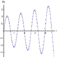
Figure 2: Left graphic: The dots represent the numerical evaluation of the inverse Laplace transform of Eq. (26). The continuous line is the approximate formula, Eq. (27). The values of the parameters are $b=\pi-0.5$ and $\varepsilon=0.1$. Right graphic: The dots represent the numerical evaluation of the inverse Laplace transform of Eq. (26). The continuous line is the approximate formula, Eq. (27). The values of the parameters are $b=\pi+0.5$ and $\varepsilon=0.1$.

4 Universality of the asymptotic equation

In this section we will find an asymptotic expression for the inverse Laplace transform of a function in the form (3). In the previous section we focused our attention on the case $P_{2}(u)$, whereas here we will predominantly consider the case $P_{1}(u)$. This case has not yet been treated since the multi-scale method essentially applies to second degree polynomials. It shall be evident that, with slight changes, the procedure can also be applied to the Fourier transform. We begin with the following relatively simple case

$$\hat{F}(u)=\frac{\hat{K}(u)}{u-z}$$ (28)

where $z$ is a complex parameter and $\hat{K}(u)$ is the Laplace transform of $K(t)$. Making the hypothesis that the Laplace transform is evaluated in $z$, that is to say $\hat{K}(z)$ exists, we may write the solution of Eq. (28) as

$$F(t)=\int_{0}^{t}K(t^{\prime})\exp[z(t-t^{\prime})]dt^{\prime}=\exp[zt]\int_{0}^{t}K(t^{\prime})\exp[-zt^{\prime}]dt^{\prime}$$ (29)

and for $t\to\infty$

$$F(t)=\exp[zt]\hat{K}(z).$$ (30)

Following the same idea we now consider a more complex form of $\hat{F}(u)$. As said in Sec. 1 a Laplace transform of the form

$$\hat{F}(u)=\frac{1}{u-z+\varepsilon\hat{K}(u)}$$ (31)

has several physical applications. As we previously assumed the function $\hat{K}(u)$ has an inverse Laplace transform, $K(t)$, and $\hat{K}(z)$ exists. Considering the time domain, Eq. (31) is equivalent to the following equation

$$\frac{d}{dt}F(t)-zF(t)=-\varepsilon\int_{0}^{t}K(t-t^{\prime})F(t^{\prime})dt^{\prime}.$$

Let us now examine Eq. (31) in more detail. Developing its denominator in $\varepsilon$ power we have

$$\hat{F}(u)=\frac{1}{u-z}\sum_{n=0}^{\infty}(-1)^{n}\frac{\varepsilon^{n}[\hat{K}(u)]^{n}}{(u-z)^{n}}.$$ (32)

Inverting the Laplace transform we obtain the following expression

$$F(t) = \sum_{n=0}^{\infty}\frac{(-1)^{n}}{n!}\int_{0}^{t}\varepsilon^{n}K_{n}(t^{\prime})(t-t^{\prime})^{n}\exp[z(t-t^{\prime})]=$$ (33)

$$= \sum_{n=0}^{\infty}\frac{(-1)^{n}}{n!}\varepsilon^{n}\frac{\partial^{n}}{\partial z^{n}}\left[\exp[zt]\int_{0}^{t}K_{n}(t^{\prime})\exp[-zt^{\prime}]dt^{\prime}\right]$$

where $K_{n}(t)$ is the $n$th convolution of $K(t)$, and in the recursive form, it is

$$K_{n}(t)=\int_{0}^{t}K(t-t^{\prime})K_{n-1}(t^{\prime})dt^{\prime},\,\,\,\,\,\,K_{0}(t)=\delta(t).$$

Since we are interested in the asymptotic behavior, we take the limit for $t\to\infty$ resulting in

$$F(t) \approx \sum_{n=0}^{\infty}\frac{(-1)^{n}}{n!}\varepsilon^{n}\frac{\partial^{n}}{\partial z}\left[\exp[zt]\int_{0}^{\infty}K_{n}(t^{\prime})\exp[-zt^{\prime}]dt^{\prime}\right]$$ (34)

$$= \sum_{n=0}^{\infty}\frac{(-1)^{n}}{n!}\varepsilon^{n}\frac{\partial^{n}}{\partial z^{n}}\left[\exp[zt]\hat{K}^{n}(z)\right]$$

where, by definition, $\hat{K}^{n}(z)\equiv[\hat{K}(z)]^{n}$. Applying simple algebra we obtain the following asymptotic expression

$$F(t)=\exp[zt]\sum_{n=0}^{\infty}\frac{(-1)^{n}}{n!}\varepsilon^{n}\left[t+\frac{\partial}{\partial z}\right]^{n}\left[\hat{K}^{n}(z)\right]\equiv\exp[zt]\phi_{1}(\varepsilon,t,z)$$ (35)

where the function $\phi_{1}(\varepsilon,t,z)$ is defined as

$$\phi_{1}(\varepsilon,t,z)=\sum_{n=0}^{\infty}\frac{(-1)^{n}}{n!}\varepsilon^{n}\left[t+\frac{\partial}{\partial z}\right]^{n}\left[\hat{K}^{n}(z)\right].$$ (36)

Note that the parameter $\varepsilon$ is not necessarily small. The only requirement is that Eq. (36) has to be a convergent series. The $\phi_{1}(\varepsilon,t,z)$ function satisfies the following equation

$$\varepsilon\frac{\partial}{\partial\varepsilon}\phi_{1}(\varepsilon,t,z)=\left[t\frac{\partial}{\partial t}+\frac{\partial^{2}}{\partial z\partial t}\right]\phi_{1}(\varepsilon,t,z).$$ (37)

Changing the variables, $\tau=\varepsilon t,\,\,v=\varepsilon$ and $w=z$, leads to a simplified version

$$\frac{\partial}{\partial v}\phi_{1}(v,w,\tau)=\frac{\partial^{2}}{\partial w\partial\tau}\phi_{1}(v,w,\tau).$$ (38)

We can further transform Eq. (38). Considering $\phi_{1}(v,w,\tau)$ as the Laplace transform of a function with respect to the variable $v$, and making the change of variables $w=x+y$ and $\tau=x-y$, we may write Eq. (38) as

$$-\lambda\Phi_{1}(s,x,y)=\left[\frac{\partial^{2}}{\partial x^{2}}-\frac{\partial^{2}}{\partial y^{2}}\right]\Phi_{1}(s,x,y)$$ (39)

where, by definition

$$\Phi_{1}(s,x,y)\equiv\frac{1}{2\pi\imath}\int\limits_{\gamma-\imath\infty}^{\gamma+\imath\infty}\phi_{1}(v,x,y)\exp[sv]dv.$$

In Eq. (39) we recognize the well known Klein-Gordon equation. Using the complex change of variables $w=x+iy$ and $\tau=x-iy$, we can rewrite Eq. (39) as

$$-\lambda\Phi_{1}(s,x,y)=\left[\frac{\partial^{2}}{\partial x^{2}}+\frac{\partial^{2}}{\partial y^{2}}\right]\Phi_{1}(s,x,y),$$ (40)

that is the Helmholtz equation. The above equations; Eqs. (38), (39) and (40), do not contain the arbitrary function $\hat{K}(z)$. This fact implies that all integro-differential equations generated by equations like Eq. (1) are driven by the same asymptotic equation. In this sense we can say that the asymptotic equation for the first order integro-differential equations is universal.

To find a more manageable expression of $\phi_{1}(\varepsilon,t,z)$, first we will rewrite it as

$$\phi_{1}(\varepsilon,t,z)=\sum_{n=0}^{\infty}\frac{(-1)^{n}}{n!}\varepsilon^{n}t^{n}\left[1+\frac{1}{t}\frac{\partial}{\partial z}\right]^{n}\left[\hat{K}^{n}(z)\right]=$$

$$=\sum_{n=0}^{\infty}\frac{(-1)^{n}}{n!}\varepsilon^{n}t^{n}\exp\left[n\log\left(1+\frac{1}{t}\frac{\partial}{\partial z}\right)\right]\left[\hat{K}(z)\right]^{n}\approx~{}$$

$$\approx\sum_{n=0}^{\infty}\frac{(-1)^{n}}{n!}\varepsilon^{n}t^{n}\exp\left[\frac{n}{t}\frac{\partial}{\partial z}\right]\left[\hat{K}(z)\right]^{n}=\sum_{n=0}^{\infty}\frac{(-1)^{n}}{n!}\varepsilon^{n}t^{n}\left[\hat{K}\left(\frac{n}{t}+z\right)\right]^{n}.$$ (41)

Under the condition that $\varepsilon$ is small enough to ensure a fast convergence of the series, in such way that only the terms $n\ll t$ contribute, we may write the following simplified expression

$$\phi_{1}(\varepsilon,t,z)\approx\sum_{n=0}^{\infty}\frac{(-1)^{n}}{n!}\varepsilon^{n}t^{n}\left[\hat{K}\left(z\right)\right]^{n}=\exp\left[-\varepsilon\hat{K}\left(z\right)t\right].$$ (42)

This implies

$$F(t)\approx\exp\left[\left(z-\varepsilon\hat{K}\left(z\right)\right)t\right],$$ (43)

and we can call this the naive solution of the problem, that is to say, the evaluation of the pole in Eq. (31) at the unperturbed value $u=z$. We stress that in general the behavior of $\phi_{1}(\varepsilon,t,z)$ as function of time is more complex than an exponential and the steps that lead from Eq. (36) to Eq. (42) confirm this statement. As an instructive example we may evaluate Eq. (36) in the case where $\hat{K}\left(z\right)=\exp[-\beta z]$. It is straightforward to obtain for $\phi_{1}(\varepsilon,t,z)$ the expression

$$\phi_{1}(\varepsilon,t,z)=\sum_{n=0}^{\infty}\frac{(-1)^{n}}{n!}\varepsilon^{n}\left[t-\beta n\right]^{n}\exp\left[-\beta nz\right].$$

The series is absolutely convergent if the inequality $\mid\!\!\varepsilon\beta\exp\left[-\beta z+1\right]\!\!\mid<1$ is satisfied.

Following the lines previously expounded for the first degree polynomial we shall find an expression for the case of a second degree polynomial. Let us consider the following Laplace transform

$$\hat{F}(u)=\frac{1}{u^{2}\pm a^{2}+\varepsilon\hat{K}(u)}.$$ (44)

For the sake of simplicity we assume that $a$ is a real parameter and we consider the plus sign in the denominator. We also need the following result

$$\mathcal{L}^{-1}\left[\frac{1}{(u^{2}+a^{2})^{n+1}}\right] = \frac{1}{a\left(2a\right)^{2n}n!}\sum_{k=0}^{n}\frac{(n+k)!}{k!(n-k)!}(2at)^{n-k}\times$$ (45)

$$\times \sin\left[at-\frac{\pi}{2}(n-k)\right].$$

Following the procedures set forth in this section we find the exact expression for $F(t)$

$$F(t) = \textrm{Im}\left[\sum_{n=0}^{\infty}\frac{(-\varepsilon)^{n}}{a\left(2a\right)^{2n}}\frac{1}{n!}\sum_{k=0}^{n}\frac{(n+k)!}{k!(n-k)!}\times\right.$$ (46)

$$\times \left.\int_{0}^{t}[-2\imath a(t-t^{\prime})]^{n-k}\exp[\imath a(t-t^{\prime})]K_{n}(t^{\prime})dt^{\prime}\right]$$

and consequently the asymptotic expression

$$F(t)\approx\textrm{Im}\left[\sum_{n=0}^{\infty}\frac{(2\imath a\varepsilon)^{n}}{a\left(2a\right)^{2n}n!}\sum_{k=0}^{n}\frac{(n+k)!}{k!(n-k)!}\frac{\partial^{n-k}}{\partial z^{n-k}}\left\{\exp[zt]\left[\hat{K}(z)\right]^{n}_{z=\imath a}\right\}\right]=$$

$$=\textrm{Im}\left[\sum_{n=0}^{\infty}\frac{(2\imath a\varepsilon)^{n}}{a\left(2a\right)^{2n}}\frac{\exp[\imath at]}{n!}\sum_{k=0}^{n}\frac{(n+k)!}{k!(n-k)!}\left[t+\frac{\partial}{\partial z}\right]^{n-k}\left[\hat{K}(z)\right]^{n}_{z=\imath a}\right].$$ (47)

Defining the function

$$\phi_{2}(\varepsilon,t,a)=\sum_{n=0}^{\infty}\frac{(2\imath a\varepsilon)^{n}}{a\left(2a\right)^{2n}}\frac{1}{n!}\sum_{k=0}^{n}\frac{(n+k)!}{k!(n-k)!}\left[t+\frac{\partial}{\partial z}\right]^{n-k}\left[\hat{K}(z)\right]^{n}_{z=\imath a}$$

we may write Eq. (47) in a more concise way

$$F(t)=\textrm{Im}\left[\exp[\imath at]\phi_{2}(\varepsilon,t,a)\right].$$

As before, a further approximated expression for $F(t)$ is given by

$$F(t) \approx \textrm{Im}\left[\exp[\imath at]\sum_{n=0}^{\infty}\frac{(2\imath a\varepsilon t)^{n}}{a\left(2a\right)^{2n}n!}\left[1+\frac{1}{t}\frac{\partial}{\partial z}\right]^{n}\left[\hat{K}(z)\right]^{n}_{z=\imath a}\right]\approx$$ (48)

$$\approx \textrm{Im}\left[\exp[\imath at]\sum_{n=0}^{\infty}\frac{(2\imath a\varepsilon t)^{n}}{a\left(2a\right)^{2n}n!}\left[\hat{K}(\frac{n}{t}+\imath a)\right]^{n}\right].$$

Finally, when $\varepsilon$ is small enough, we rediscover the naive solution

$$F(t) \approx \textrm{Im}\left[\frac{\exp\left[\imath a\left(1+\varepsilon\frac{K(\imath a)}{2a^{2}}\right)t\right]}{a}\right]=$$ (49)

$$= \frac{\exp\left[\imath a\left(1+\varepsilon\frac{\hat{K}(\imath a)}{2a^{2}}\right)t\right]-\exp\left[-\imath a\left(1+\varepsilon\frac{\hat{K}(-\imath a)}{2a^{2}}\right)t\right]}{2\imath a}$$

that basically coincides with Eq. (23). As for $\phi_{1}(\varepsilon,t,z)$, the function $\phi_{2}(\varepsilon,t,a)$ does not merely represent an exponential correction to the exponential unperturbed solution. As previously stated, it is more complex. Note that the exponential correction holds true only for a sufficiently small $\varepsilon$.

5 Physical applications: the convoluted Lindblad equation

A wide range of applications exists for first and second order integro-differential equations. In this section we shall study a case that is well known in the scientific literature for the quantum density matrix, the celebrated Lindblad equation [9]. We begin with

$$\frac{\partial}{\partial t}\rho(t)=-\frac{\imath}{\hbar}[H,\rho(t)]-L_{D}\rho(t)$$ (50)

where $L_{D}$ is a positive semidefinite Lindblad operator of the form [10]

$$L_{D}\rho=\frac{1}{\tau_{D}}[q,[q,\rho]]$$

with $q$ being the system s variable measured by the environment, while $\tau_{D}$ represents the time scale of the environment-induced measurement. The Hamiltonian $H$ and the observable $q$ are properties of the system of interest, and they are operators, as prescribed by quantum mechanics. To reduce the number of parameters, we will set $\hbar=1$. For systems driven by a time independent Hamiltonian, Eq. (50) can be promptly solved

$$\rho(t)=\exp[Lt]\rho(0)=\sum_{k=1}^{n}c_{k}\exp[\lambda_{k}t]\rho_{k}$$ (51)

where $L=-\imath[H,\cdot]-L_{D}$ is the total liouvillian, $\rho_{k}$ are its eigenvectors and $\lambda_{k}$ its eigenvalues. If the matrix is an infinite dimensional matrix the sum can be extended to the infinite. A natural generalization of Eq. (50) is

$$\frac{\partial}{\partial t}\rho(t)=\int_{0}^{t}\Phi(t-t^{\prime})L\rho(t^{\prime})dt^{\prime}.$$ (52)

Barnett and Stenholm [13] studied the above equation considering the system as a harmonic oscillator embedded in a reservoir. They showed that, even utilizing a simple exponential kernel, the density matrix is positive definite only for a short time. Wilkie previously [14] showed that adding to Eq. (52) an inhomogeneous term with well defined characteristic, the positivity properties of $\rho(t)$ are preserved. Recently Bologna et al. [15] demonstrated that it is always possible to build a positive definite density matrix using the discrete version of the Lindblad equation as a starting point. The passage from natural time $n$ to continuous time $t$ is obtained performing the subordination of the density matrix derived from the discrete equation.

Starting from Eq. (52) it is still an open problem to find conditions on the kernel $\Phi(t)$ that generate a positive definite matrix. To achieve this, we rewrite the kernel operator making a dimensionless parameter $\varepsilon$ explicit, so that $\Phi(t-t^{\prime})L\to\varepsilon\Phi(t-t^{\prime})L$. Then we evaluate the Laplace transform of Eq. (52)

$$\hat{\rho}(u)=\left[u-\varepsilon\hat{\Phi}(u)L\right]^{-1}\rho(0)$$ (53)

where $\hat{\Phi}(u)$ is the Laplace transform of $\Phi(t)$. When the inverse of the operator $u-\varepsilon\hat{\Phi}(u)L$ acts on the density matrix it can be written in terms of the eigenvalues of $L$, namely

$$\frac{1}{u-\varepsilon\hat{\Phi}(u)L}\rho(0)=\sum_{k=1}^{n}\frac{c_{k}}{u-\varepsilon\hat{\Phi}(u)\lambda_{k}}\rho_{k}.$$

Each addend of the sum is a Laplace transform of the form of Eq. (31) with $z=0$ and the developing parameter parameter $\bar{\varepsilon}_{k}\equiv\varepsilon\lambda_{k}$. Note that $\bar{\varepsilon}_{k}$ is a linear function of the eigenvalues. In principle, using the results of Sec. 4, and when $\varepsilon$ is small enough, we can write the inverse Laplace transform as

$$\rho(t)=\sum_{k=1}^{n}c_{k}\exp[\varepsilon\lambda_{k}\hat{\Phi}(0)t]\rho_{k}.$$ (54)

As proven in Ref. [10], the density matrix given by Eq. (51) has the proper physical meaning as does the matrix given by Eq. (54) since the only difference between the two is the time scale factor $\varepsilon\hat{\Phi}(0)$. But, the application of the method developed in Sec. 4 has to be carefully considered. As stressed several times, $\varepsilon$ has to be small enough, one must count the factors in front of it, in order to apply the naive solution. More precisely the following sufficient conditions apply:
i) $\mid\!\!\hat{\Phi}(0)\!\!\mid<\infty$.
ii) $\hat{\Phi}(0)>0$.
iii) $\varepsilon\mid\!\!\lambda_{k}\!\!\mid\ll 1\,\,\textrm{for}\,\,k=1,2,\cdots$.
The reasons for the above conditions rest on the following arguments: Condition (i) is due to the requirement that in general  $\hat{\Phi}(z)$ has to exist and consequently $\hat{\Phi}(0)$ has to exist (see discussion in Sec. 4). Condition (ii) is required to preserve the sign at the exponent in the exponential function [compare Eq. (51) with Eq. (54)]. Condition (iii) ensures a small developing parameter. To insure a faster numerical convergence, condition (iii) may be substituted with the more convenient one
iv) $\varepsilon\hat{\Phi}(0)\mid\!\!\lambda_{k}\!\!\mid\ll 1\,\,\textrm{for}\,\,k=1,2,\cdots$.
Considering the case studied in Ref. [13] and applying the criteria of condition (iii), we should select a value of $\varepsilon$ sufficiently small such that $\varepsilon\!\mid\!\!\lambda_{k}\!\!\mid\ll 1$ $\forall k$. The results of Ref. [13] show that the eigenvalues are linearly divergent as a function of the index, viz. $\lambda_{k}\sim k$, so that condition (iii), $\varepsilon\mid\!\!\lambda_{k}\!\!\mid\ll 1$, can never be satisfied and the naive solution is not applicable. The density matrix evaluated in Ref. [13] is not a positive definite matrix. We conclude that this is due to the divergent structure of its eigenvalues.

To elucidate this last point, we can consider a finite-dimensional density matrix where the condition $\mid\!\!\lambda_{k}\!\!\mid\leq M$ $\forall k$, with $M$ as a finite positive number, can be satisfied. The simplest case is a $2\times 2$ density matrix. Strictly speaking, to keep the analogy with the infinite dimensional case studied in Ref. [13] we should consider the convolution of the following equation

$$\frac{\partial}{\partial t}\rho(t)=-\frac{1}{\tau}[\sigma_{x},[\sigma_{x},\rho(t)]]$$ (55)

where the operator $q$ has been identified with Pauli’s matrix $\sigma_{x}$. It is straightforward to show that the convolution of the right side of Eq. (55) with an exponential, always produces a positive definite density matrix. We shall test the results of Sec. 4 considering the convolution of the equation containing the full liouvillian used in Ref. [15],

$$\frac{\partial}{\partial t}\rho(t)=L\rho(t)=-\imath\omega[\sigma_{x},\rho(t)]-\frac{1}{\tau}[\sigma_{z},[\sigma_{z},\rho(t)]]$$ (56)

where $\sigma_{x}$ and $\sigma_{z}$ are Pauli’s matrices. The convoluted version of Eq. (56) may be written as

$$\frac{\partial}{\partial t}\rho(t)=\varepsilon\int_{0}^{t}\Phi(t-t^{\prime})L\rho(t^{\prime})dt=\varepsilon\int_{0}^{t}\exp[-\gamma(t-t^{\prime})]L\rho(t^{\prime})dt$$ (57)

where $\varepsilon$ is a dimensionless parameter. The above equation admits an analytical solution. We shall focus on the diagonal element $\rho_{11}(t)$ since $\rho_{22}(t)$ can be derived via the relation $\rho_{11}(t)+\rho_{22}(t)=1$. Taking into account that the eigenvalues of the liouvillian operator $L$ are

$$\lambda_{1}=-\frac{4}{\tau},\,\,\,\,\lambda_{2}=\frac{2\left(-1-\sqrt{1-\tau^{2}\omega^{2}}\right)}{\tau},\,\,\,\,\lambda_{3}=\frac{2\left(-1+\sqrt{1-\tau^{2}\omega^{2}}\right)}{\tau},\,\,\,\,\lambda_{4}=0,$$

and assuming as the initial condition $\rho_{11}(0)=1$, we have

$$\rho_{11}(t) = \frac{1}{2}+\frac{e^{-\frac{t\gamma}{2}}}{4\Gamma_{1}}\left(1-\frac{1}{\sqrt{1-\tau^{2}\omega^{2}}}\right)\left(\Gamma_{1}\cosh\left[\frac{t\Gamma_{1}}{2\tau}\right]+\gamma\tau\sinh\left[\frac{t\Gamma_{1}}{2\tau}\right]\right)+$$ (58)

$$+ \frac{e^{-\frac{t\gamma}{2}}}{4\Gamma_{2}}\left(1+\frac{1}{\sqrt{1-\tau^{2}\omega^{2}}}\right)\left(\Gamma_{2}\cosh\left[\frac{t\Gamma_{2}}{2\tau}\right]+\gamma\tau\sinh\left[\frac{t\Gamma_{2}}{2\tau}\right]\right)$$

where we defined the quantities $\Gamma_{1}$ and $\Gamma_{2}$ as

$$\Gamma_{1}=\sqrt{\tau\left(-8\varepsilon+\gamma^{2}\tau-8\varepsilon\sqrt{1-\tau^{2}\omega^{2}}\right)},\,\,\,\,\Gamma_{2}=\sqrt{\tau\left(-8\varepsilon+\gamma^{2}\tau+8\varepsilon\sqrt{1-\tau^{2}\omega^{2}}\right)}.$$

From Eq. (58) we can deduce that, in general, $\rho_{11}(t)$ is neither a positive quantity $\forall t$ nor a quantity smaller than the unit $\forall t$. Applying the method developed in Sec. 4, the analysis of the eigenvalues shows that there are two cases of interest: $\tau\omega<1$ corresponding to real eigenvalues, and $\tau\omega>1$ corresponding to complex eigenvalues. To simplify the two cases, consider $\tau\omega\ll 1$ and $\tau\omega\gg 1$. In the first case, condition (iv) may be written as

$$\frac{4\varepsilon}{\gamma\tau}\ll 1$$ (59)

whereas in the second case it may be written as

$$\frac{2\varepsilon\omega}{\gamma}\ll 1.$$ (60)

Fig. 3 shows the plot of $\rho_{11}(t)$ for given values of the parameters $\varepsilon,\,\,\omega,\,\,\tau,\,\,\gamma$. In the left graphic, condition (60) is violated because $2\varepsilon\omega/\gamma\approx 2.1$, and $\rho_{11}(t)$ does not have physical meaning. In the right graphic, on the contrary, condition (60) is satisfied as $2\varepsilon\omega/\gamma\approx 0.14$, and $\rho_{11}(t)$ is a positive function smaller then the unit $\forall t$.

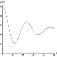
Figure 3: Left graphic: The plot of $\rho_{11}(t)$, Eq. (58). The value of the parameters are: $\epsilon=1.5,\,\,\gamma=8,\,\,\tau=1$ and $\omega=5.5$ so that $2\varepsilon\omega/\gamma\approx 2.1$. Right graphic: The continuous line represents the plot of $\rho_{11}(t)$, Eq. (58), while the dashed line represents the plot of the approximate solution, Eq. (54). The value of the parameters are: $\epsilon=0.1,\,\,\gamma=8,\,\,\tau=1$ and $\omega=5.5$ so that $2\varepsilon\omega/\gamma\approx 0.14$.

6 Conclusions

This paper introduced a procedure to obtain an analytical asymptotic expression for the solution of first and second order integro-differential equations containing an arbitrary kernel. We found an asymptotic expression for the correspondent inverse Laplace and Fourier transforms containing an arbitrary function $\hat{K}(u)$. It was shown that a first order integro-differential equation is asymptotically driven by an equation that is independent from the specific form of the kernel of the integro-differential equation. A general expression for the desired asymptotic solution was also given. This result was applied to the convoluted version of the Lindblad equation explaining why even a simple kernel, such as an exponential function, does not generate a positive definite density matrix. Sufficient conditions on the kernel function so as to generate a positive definite density matrix were given at the end of Sec. 5. Indeed, these conditions showed that the structure of the eigenvalues of the liouvillian operator plays a crucial role in determining the positivity of the density matrix.

References

References

[1]Bellman R. E. and Roth R. S., The Laplace Transform (World
Scientific, Singapore, 1984).
[2]Berberan-Santos M. N., J. Math. Chem.38, 165 (2005)
[3]
Davies B. and Martin B., J. Comput. Phys.1,1
(1979)
[4]Fox R. F., J. Math. Phys.18,2331 (1977)
[5]Ferrario M. and Grigolini P., J. Math. Phys.20, 2567 (1978)
[6]Grigolini P., J. Stat. Phys.27,283 (1982)
[7]Hong J. and Lee H., Phys. Rev. Lett.55,2375 (1985)
[8]Hong J. and Lee H., Phys. Rev. Lett.70,1972 (1993)
[9]Lindblad G., Commun. Math. Phys.48, 119
(1976)
[10]
Gorini V., Kossakovski A., and Sudarshan E. C. G., J. Math.
Phys.17, 821 (1976)
[11]Fetter A. L. and Walecka J. D.,
Quantum Theory of Many-Particle Systems, McGraw-Hill,
New York
[12]Kevorkian J. and Cole J. D.,
Multiple Scale and Singular Perturbation Methods ,
Springer-Verlag New York (1996)
[13]Barnett S.
M. and Stenholm S., Phys. Rev. A 64, 033808 (2001).
[14]Wilkie J., Phys. Rev. E62, 8808 (2000)
[15]
Bologna M., Budini A., Giraldi F. and Grigolini P., J. Chem.
Phys.130, 244106 (2009)