Direct numerical simulations of statistically steady, homogeneous, isotropic fluid turbulence with polymer additives

Abstract

We carry out a direct numerical simulation (DNS) study that reveals the effects of polymers on statistically steady, forced, homogeneous, isotropic fluid turbulence. We find clear manifestations of dissipation-reduction phenomena: On the addition of polymers to the turbulent fluid, we obtain a reduction in the energy dissipation rate, a significant modification of the fluid energy spectrum, especially in the deep-dissipation range, signatures of the suppression of small-scale structures, including a decrease in small-scale vorticity filaments. We also compare our results with recent experiments and earlier DNS studies of decaying fluid turbulence with polymer additives.

I Introduction

The addition of small amounts of polymers to a turbulent fluid leads to dramatic changes that include modifications of the small-scale properties of the flow hoy77 ; kal_poly04 ; per06 and, in wall-bounded flows, the phenomenon of drag reduction toms49 ; lum73 ; vir75 , in which polymer additives allow the maintenance of a given flow rate at a lower pressure gradient than is required without these additives. Several experimental, numerical, and analytical studies have investigated drag reduction vir75 ; lum73 ; too97 ; dub01 ; pta01 ; pta03 ; lvo04 ; ang05 ; pro08 in wall-bounded flows. These studies have shown that the addition of polymers modifies the turbulence significantly in the region near the wall; and this leads to an increase in the mean velocity in the bulk. By contrast, there have been only some investigations of the effects of polymer additives on homogeneous, isotropic turbulence. Examples include recent experiments oue09 ; lib05 ; lib06 , which have been designed to obtain a high degree of isotropy in the turbulent flow, and shell-model studies and direct numerical simulations (DNS) ben03 ; vai03 ; kal_poly04 ; ang05 ; per06 . These studies have shown that the addition of polymers to a turbulent flow leads to a considerable reduction in small-scale structures; and they have also discovered the phenomenon of dissipation reduction, namely, a reduction in the energy dissipation rate $\epsilon$, in decaying turbulence kal_poly04 ; per06 . In this paper we first elucidate the phenomenon of dissipation reduction for the case of statistically steady, homogeneous, isotropic turbulence with polymer additives; we then study the small-scale properties of such flows.

We do this by conducting a series of high-resolution DNS studies of the three-dimensional Navier-Stokes equation coupled to an equation for the polymer conformation tensor, which describes the polymer additives at the level of the FENE-P kal_poly04 ; per06 model. Before we give the details of our study, it is useful to summarise our principal results; these are in two parts.

The first part contains results from our DNS of forced, statistically steady, fluid turbulence, with polymer additives, at moderate Reynolds numbers ($Re_{\lambda}\simeq 80$). The forcing is chosen such that the energy injected into the fluid remains fixed lam05 , both with and without polymers; this mimics the forcing scheme used in the experiments of Ref. lib05 ; lib06 . We find that, on the addition of polymers, the energy in the statistically steady state and the energy-dissipation rate are reduced. This dissipation reduction increases with an increase in the polymer concentration $c$ at fixed Weissenberg number $We$, the ratio (see Table 1) of the polymer time scale $\tau_{\rm P}$ to a shearing time scale in the turbulent fluid. The dissipation reduction also increases with $We$ if we hold $c$ fixed. The dissipation reduction seen in our simulations should not be confused with the phenomenon of drag reduction seen in wall-bounded flows. In the fluid energy spectrum we find that the energy content increases marginally at small wavevectors on the addition of polymers, but it decreases for intermediate wavevectors. In this part of our study we use $256^{3}$ collocation points and attain a moderate Reynolds numbers $Re_{\lambda}\simeq 80$; but we do not resolve the deep-dissipation range. (We consider the deep dissipation range in the following paragraph.) We also obtain the structural properties of the fluid with and without polymers and show that polymers suppress large-vorticity and large-strain events; our results here are in qualitative agreement with the experiments of Ref. lib05 ; lib06 . Furthermore, we find, as in our study of decaying turbulence per06 , that the polymer extension increases with an increase in the polymer relaxation time $\tau_{\rm P}$. We compare our results, e.g., those for the energy spectrum, with their counterparts in our earlier study of decaying fluid turbulence with polymer additives per06 . In such comparisons, we use averages over the statistically steady state of our system here; and, for the case of decaying turbulence, we use data obtained at the cascade-completion time, at which a plot of the energy dissipation rate versus time displays a maximum.

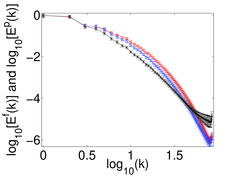
In the second part of our study we carry out the highest-resolution DNS, attempted so far, of forced, statistically steady, fluid turbulence with polymer additives; we drive the fluid by an external, stochastic force as in Ref. esw88 . This part of our study has been designed to uncover the effects of polymers on the deep-dissipation range, so the Reynolds numbers is small ($Re_{\lambda}\simeq 16$). By comparing fluid energy spectra, with and without polymers, we find that the polymers suppress the energy in the dissipation range but increase it in the deep-dissipation range. Finally, we calculate the second-order velocity structure function $S_{2}(r)$ directly from the energy spectrum via a Fourier transformation; this shows that $S_{2}(r)$ with polymers is smaller than $S_{2}(r)$ without polymers in this range.

The remaining part of this paper is organised as follows. In Section II we present the equations we use for the polymer solution and describe, in subsection II.1, the method we use for the numerical integration of these equations. Section III is devoted to a discussion of our results; as we have mentioned above, these are divided into two parts; the first part is contained in subsections III.1-III.3 and the second in subsection III.4. Section IV contains a concluding discussion.

II Equations and Numerical Methods

We model a polymeric fluid solution by using the three-dimensional, Navier-Stokes (NS) equations for the fluid coupled with the Finitely Extensible Nonlinear Elastic-Peterlin (FENE-P) equation for the polymer additives per06 . The polymer contribution to the fluid is modelled by an extra stress term in the NS equations. The FENE-P equation approximates a polymer molecule by a nonlinear dumbbell, which has a single relaxation time and an upper bound on the maximum extension. The NS and FENE-P (henceforth NSP) equations are

$$D_{t}{\bf u} = \nu\nabla^{2}{\bf u}+\frac{\mu}{\tau_{\rm P}}\nabla.[f(r_{\rm P}){\cal C}]-{\nabla}p+{\bf f};$$ (1)

$$D_{t}{\cal C} = {\cal C}.(\nabla{\bf u})+{(\nabla{\bf u})^{T}}.{\cal C}-\frac{{f(r_{\rm P}){\cal C}}-{\cal I}}{\tau_{\rm P}}.$$ (2)

Here ${{\bf u}({\bf x},t)}$ is the fluid velocity at point ${\bf x}$ and time $t$, incompressibility is enforced by $\nabla.{\bf u}=0$, $D_{t}=\partial_{t}+{\bf u}.\nabla$, $\nu$ is the kinematic viscosity of the fluid, $\mu$ the viscosity parameter for the solute (FENE-P), $\tau_{\rm P}$ the polymer relaxation time, $\rho$ the solvent density (set to $1$), $p$ the pressure, ${{\bf f}({\bf x},t})$ the external force at point ${\bf x}$ and time $t$, $(\nabla{\bf u})^{T}$ the transpose of $({\nabla{\bf u}})$, ${\cal C}_{\alpha\beta}\equiv{\langle{R_{\alpha}}{R_{\beta}}\rangle}$ the elements of the polymer-conformation tensor ${\cal C}$ (angular brackets indicate an average over polymer configurations), ${\cal I}$ the identity tensor with elements $\delta_{\alpha\beta}$, $f(r_{\rm P})\equiv{(L^{2}-3)/(L^{2}-r_{\rm P}^{2})}$ the FENE-P potential that ensures finite extensibility, $r_{\rm P}\equiv\sqrt{Tr(\cal C)}$ and $L$ the length and the maximum possible extension, respectively, of the polymers, and $c\equiv\mu/(\nu+\mu)$ a dimensionless measure of the polymer concentration vai03 ; $c=0.1$ corresponds, roughly, to $100$ppm for polyethylene oxide vir75 . Table 1 lists the parameters of our simulations.

	$N$	$\delta{t}$	$L$	$\nu$	$\tau_{\rm P}$	$c$	$We$
NSP-256A	$256$	$5.0\times 10^{-4}$	$100$	$5\times 10^{-3}$	$0.5$	$~{}0.1$	$3.5$
NSP-256B	$256$	$5.0\times 10^{-4}$	$100$	$5\times 10^{-3}$	$1.0$	$~{}0.1$	$7.1$
NSP-512	$512$	$10^{-3}$	$100$	$5\times 10^{-2}$	$1.0$	$0.1$	$0.9$

Table 1: The cube root $N$ of the number of collocation points, the time step $\delta t$, the maximum possible polymer extension $L$, the kinematic viscosity $\nu$, the polymer-relaxation time $\tau_{\rm P}$, and the polymer concentration parameter $c$ for our four runs ${\tt NSP-256A}$, ${\tt NSP-256B}$ and ${\tt NSP-512}$. We also carry out DNS studies of the NS equation with the same numerical resolutions as in our NSP runs. The Taylor-microscale Reynolds number $Re_{\lambda}\equiv\sqrt{20}{\mathcal{E}^{\rm f}}/\sqrt{3\nu\epsilon^{\rm f}_{\nu}}$ and the Weissenberg number $We\equiv\tau_{\rm P}\sqrt{\epsilon^{\rm f}_{\nu}/\nu}$ are as follows: ${\tt NSP-256A}$ and ${\tt NSP-256B}$: $Re_{\lambda}\simeq 80$ and ${\tt NSP-512}$: $Re_{\lambda}\simeq 16$; the Kolmogorov dissipation length scale $\eta\equiv(\nu^{3}/\epsilon^{\rm f}_{\nu})^{1/4}$. For our runs ${\tt NSP-256A-B}$, $\eta\simeq 1.07\delta x$; and for run ${\tt NSP-512}$, $\eta\simeq 19\delta x$, where $\delta x\equiv{\mathbb{L}}/N$ is the grid resolution of our simulations. The integral length scale $l_{\rm int}\equiv(3\pi/4)\sum k^{-1}E(k)/(\sum E(k))$ and $T_{\rm eddy}\equiv u_{\rm rms}/l_{\rm int}$ are as follows: ${\tt NSP-256A}$ and ${\tt NSP-256B}$: $l_{\rm int}\simeq 1.3$ and $T_{\rm eddy}\simeq 1.2$; and, for ${\tt NSP-512}$, $l_{\rm int}\simeq 2.05$ and $T_{\rm eddy}\simeq 4.0$.

II.1 Numerical Methods

We consider homogeneous, isotropic, turbulence, so we use periodic boundary conditions and solve Eq. (1) by using a pseudospectral method Can88 ; vin91 . We use $N^{3}$ collocation points in a cubic domain (side ${\mathbb{L}}=2\pi$). We eliminate aliasing errors by the 2/3 rule Can88 ; vin91 , to obtain reliable data at small length scales; and we use a second-order, slaved, Adams-Bashforth scheme for time marching. In earlier numerical studies of homogeneous, isotropic turbulence with polymer additives it has been shown that sharp gradients are formed during the time evolution of the polymer conformation tensor; this can lead to dispersion errors vai03 ; vai06 . To avoid these dispersion errors, shock-capturing schemes have been used to evaluate the polymer-advection term $[{({\bf u}\cdot\nabla){\mathcal{C}}}]$ in Ref. vai06 . In our simulations we have modified the Cholesky-decomposition scheme of Ref. vai03 , which preserves the symmetric positive definite nature of the tensor ${\mathcal{C}}$. We incorporate the large gradients of the polymer conformation tensor by evaluating the polymer-advection term $[{({\bf u}\cdot\nabla)\ell}]$ via the Kurganov-Tadmor shock-capturing scheme kt00 . For the derivatives on the right-hand side of Eq. (2) we use an explicit, fourth-order, central-finite-difference scheme in space; and the temporal evolution is carried out by using an Adams-Bashforth scheme. The numerical error in $r_{\rm P}$ must be controlled by choosing a small time step $\delta t$, otherwise $r_{\rm P}$ can become larger than $L$, which leads to a numerical instability; this time step is much smaller than what is necessary for a pseudospectral DNS of the NS equation alone. Table 1 lists the parameters we use. We preserve the symmetric-positive-definite (SPD) nature of $\cal C$ at all times by using vai03 the following Cholesky-decomposition scheme: If we define

$${\cal J}\equiv f(r_{\rm P}){\cal C},$$ (3)

Eq. (2) becomes

$$D_{t}{\cal J}={\cal J}.(\nabla{\bf u})+({\nabla\bf u})^{T}.{\cal J}-s({\cal J}-{\cal I})+q{\cal J},$$ (4)

where

$$s = \frac{L^{2}-3+j^{2}}{\tau_{\rm P}L^{2}},$$

$$q = \frac{d/(L^{2}-3)-(L^{2}-3+j^{2})(j^{2}-3)}{(\tau_{\rm P}L^{2}(L^{2}-3))},$$

$$j^{2} \equiv Tr({\cal J}),{\rm and}$$

$$d = Tr[{\cal J}.(\nabla{\bf u})+(\nabla{\bf u})^{T}.{\cal J}].$$

${\cal C}$ and hence ${\cal J}$ are SPD matrices; we can, therefore, write ${\cal J}={\cal LL}^{T}$, where ${\cal L}$ is a lower-triangular matrix with elements $\ell_{ij}$, such that $\ell_{ij}=0$ for $j>i$, and

$$\mathcal{J}\equiv\left(\begin{array}[]{ccc}\ell_{11}^{2}&\ell_{11}\ell_{21}&\ell_{11}\ell_{31}\\ \ell_{11}\ell_{21}&\ell_{21}^{2}+\ell_{22}^{2}&\ell_{21}\ell_{31}+\ell_{22}\ell_{32}\\ \ell_{11}\ell_{31}&\ell_{21}\ell_{31}+\ell_{22}\ell_{32}&\ell_{31}^{2}+\ell_{32}^{2}+\ell_{33}^{2}\end{array}\right).$$ (5)

Equation (4) now yields $(1\leq i\leq 3$ and $\Gamma_{ij}=\partial_{i}u_{j})$ the following set of equations:

$${D_{t}\ell_{i1}} = \sum_{k}\Gamma_{ki}\ell_{k1}+\frac{1}{2}\Big{[}(q-s)\ell_{i1}+(-1)^{(i\bmod 1)}\frac{s\ell_{i1}}{\ell^{2}_{11}}\Big{]}$$

$${}+(\delta_{i3}+\delta_{i2})\frac{\ell_{i2}}{\ell_{11}}\sum_{m>1}\Gamma_{m1}\ell_{m2}$$

$${}+\delta_{i3}\Gamma_{i1}\frac{\ell^{2}_{33}}{\ell_{11}},~{}\mbox{for}~{}i\geq 1;$$

$${D_{t}\ell_{i2}} = \sum_{m\geqslant 2}\Gamma_{mi}\ell_{m2}-\frac{\ell_{i1}}{\ell_{11}}\sum_{m\geqslant 2}\Gamma_{m1}\ell_{m2}$$

$${}+\frac{1}{2}\Big{[}(q-s)\ell_{i2}+(-1)^{(i+2)}s\frac{\ell_{i2}}{\ell_{22}^{2}}\Big{(}1+\frac{\ell^{2}_{21}}{\ell^{2}_{11}}\Big{)}\Big{]}$$

$${}+\delta_{i3}\Big{[}\frac{\ell^{2}_{33}}{\ell_{22}}\Big{(}\Gamma_{32}-\Gamma_{31}\frac{\ell_{21}}{\ell_{11}}\Big{)}+s\frac{\ell_{21}\ell_{31}}{\ell^{2}_{11}\ell_{22}}\Big{]},~{}\mbox{for}~{}i\geq 2;$$

$${D_{t}\ell_{33}} = \Gamma_{33}\ell_{33}-\ell_{33}\Big{[}\sum_{m<3}\frac{\Gamma_{3m}\ell_{3m}}{\ell_{mm}}\Big{]}+\frac{\Gamma_{31}\ell_{32}\ell_{21}\ell_{33}}{\ell_{11}\ell_{22}}$$ (6)

$${}-s\frac{\ell_{21}\ell_{31}\ell_{32}}{\ell^{2}_{11}\ell_{22}\ell_{33}}+\frac{1}{2}\Big{[}(q-s)\ell_{33}$$

$${}+\frac{s}{\ell_{33}}\Big{(}1+\sum_{m<3}\frac{\ell^{2}_{3m}}{\ell^{2}_{mm}}\Big{)}+\frac{s\ell^{2}_{21}\ell^{2}_{32}}{\ell^{2}_{11}\ell^{2}_{22}\ell_{33}}\Big{]}.$$

The SPD nature of $\cal C$ is preserved by Eqs. (6) if $\ell_{ii}>0$, which we enforce explicitly vai03 by considering the evolution of $\ln(\ell_{ii})$ instead of $\ell_{ii}$.

We resolve the sharp gradients in the polymer conformation tensor by discretizing the polymer advection term by using the Kurganov-Tadmor scheme kt00 . Below we show the discretization of the advection term $u\partial_{x}\ell$, where ${\bf u}\equiv(u,v,w)$ and $\ell$ is one of the components of the $\ell_{\alpha\beta}$; the discretization of the other advection terms in Eq. (6) is similar.

$$u\partial_{x}\ell = \frac{H_{i+1/2,j,k}-H_{i-1/2,j,k}}{\delta x},$$

$$H_{i+1/2,j,k} = \frac{u_{i+1/2,j,k}[\ell_{i+1/2,j,k}^{+}+\ell_{i+1/2,j,k}^{-}]}{2}$$

$$-\frac{a_{i+1/2,j,k}[\ell_{i+1/2,j,k}^{+}-\ell_{i+1/2,j,k}^{-}]}{2},$$

$$\ell_{i+1/2,j,k}^{\pm} = \ell_{i+1,j,k}\mp\frac{\delta x}{2}(\partial_{x}\ell)_{i+1/2\pm 1/2,j,k}\;,$$

$$a_{i+1/2,j,k} \equiv |u_{i+1/2,j,k}|\;,$$ (7)

where $i,j,k=0,\ldots(N-1)$ denote the grid points and $\delta x=\delta y=\delta z$ is the grid spacing along the three directions.

We use the following initial conditions (superscript $0$): ${\cal C}^{0}_{mn}({\bf x})=\delta_{mn}$ for all ${\bf x}$; and ${u}^{0}_{m}({\bf k})=P_{mn}({\bf k}){v}^{0}_{n}({\bf k})\exp(\iota{\theta_{n}(\bf{k})})$, with $m,n=x,y,z$, $P_{mn}=(\delta_{mn}-k_{m}k_{n}/k^{2})$ the transverse projection operator, ${\bf k}$ the wave vector with components $k_{m}=(-N/2,-N/2+1,\ldots,N/2)$ and magnitude $k=|{\bf k}|$, $\theta_{n}({\bf k})$ random numbers distributed uniformly between $0$ and $2\pi$, and $v^{0}_{n}({\bf k})$ chosen such that the initial kinetic-energy spectrum is $E^{0}(k)=k^{4}\exp(-2.0{k}^{2})$. This initial condition corresponds to a state in which the fluid energy is concentrated, to begin with, at small $k$ (large length scales); and the polymers are in a coiled state. Our simulations are run for $45T_{\rm eddy}$ and a statistically steady state is reached in roughly $10T_{\rm eddy}$, where the integral-scale, eddy-turnover time $T_{\rm eddy}\equiv u_{\rm rms}/l_{\rm int}$, with $u_{\rm rms}$ the root-mean-square velocity and $l_{\rm int}\equiv\sum_{k}k^{-1}E(k)/\sum_{k}E(k)$ the integral length scale. Along with our runs ${\tt NSP-256A}$ and ${\tt NSP-256B}$ we also carry out pure-fluid, NS simulations till a statistically steady state is reached; this takes about $10-15T_{\rm eddy}$. Once this pure-fluid simulation reaches a statistically steady state, we add polymers to the fluid at $27T_{\rm eddy}$; i.e., beyond this time we solve the coupled NSP equations 1 and 2 by using the methods given above. We then allow $5-6T_{\rm eddy}$ to elapse, so that transients die down, and then we collect data for fluid and polymer statistics for another $25T_{\rm eddy}$ for our runs ${\tt NSP-256A}$ and ${\tt NSP-256B}$.

III Results

We now present the results that we have obtained from our DNS. In addition to ${\bf u}({\bf x},t)$, its Fourier transform ${\bf u}_{\bf k}(t)$, and ${\cal C}({\bf x},t)$, we monitor the vorticity ${\bm{\omega}}\equiv\nabla\times{\bf u}$, the kinetic-energy spectrum $E(k,t)\equiv\sum_{k-1/2<k^{\prime}\leq k+1/2}|{\bf u}^{2}_{\bf k^{\prime}}(t)|$, the total kinetic energy  ${\mathcal{E}}(t)\equiv\sum_{k}E(k,t)$, the energy-dissipation-rate $\epsilon_{\nu}(t)\equiv\nu\sum_{k}k^{2}E(k,t)$, the probability distribution of scaled polymer extensions $P(r_{\rm P}^{2}/L^{2})$, the PDF of the strain and the modulus of the vorticity, and the eigenvalues of the strain tensor. For notational convenience, we do not display the dependence on $c$ explicitly. In subsection III.1 we present the time evolution of $E$ and $\epsilon_{\nu}$ and provide evidence for dissipation reduction by polymer additives. This is followed by subsections III.2 and III.3 that deal, respectively, with the effects of polymers on fluid energy spectra and small-scale structures in turbulent flows. In subsection III.4 we examine the modification, by polymer additives, of fluid-energy spectra in the deep dissipation range.

III.1 The Energy and its Dissipation Rate

We first consider the effects of polymer additives on the time evolution of the fluid energy $E$ for our runs ${\tt NSP-256A}$ and ${\tt NSP-256B}$; this is shown in Fig. 1. The polymers are added to the fluid at $t=27T_{\rm eddy}$. The addition of polymers leads to a new statistically steady state; specifically, we find for $We=3.5$ and $We=7.1$, that the average energy of the fluid with polymers is reduced in comparison to the average energy of the fluid without polymers.

Figure 1: (Color online) A plot of the fluid energy $E$ versus the dimensionless time $t/T_{\rm eddy}$ (runs NSP-256A and NSP-256B) for Weissenberg numbers $We=3.5$ (blue circles) and $We=7.1$ (black dashed line). The corresponding plot for the pure-fluid case is also shown for comparison (red line). The polymers are added to the fluid at $t=27T_{\rm eddy}$.

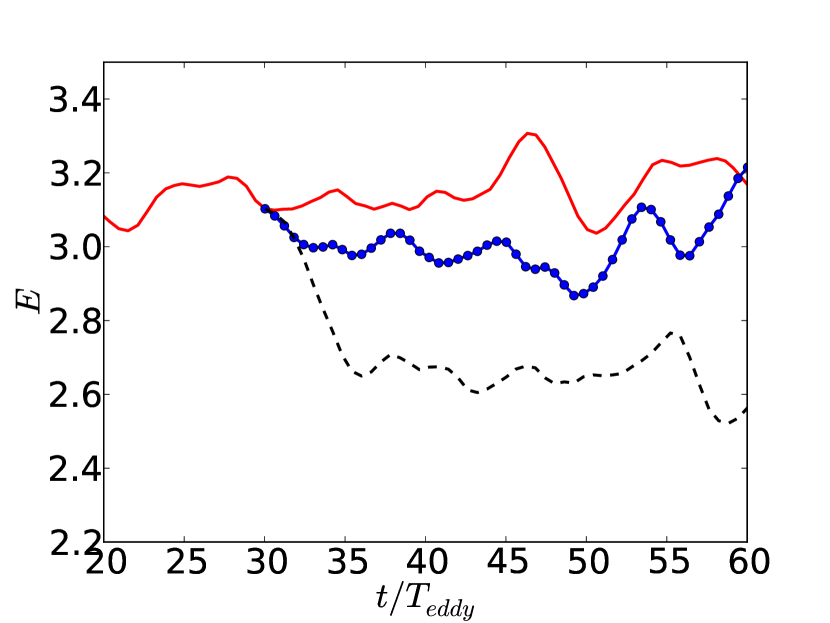
By using Eq. (1), we obtain the following energy-balance equation for the fluid with polymer additives:

$$\frac{dE}{dt} = \epsilon_{\nu}+\epsilon_{\rm poly}+\epsilon_{\rm inj},$$ (8)

$$\epsilon_{\nu} = -\nu\frac{1}{V}\int{\bf u}\cdot\nabla^{2}{\bf u},$$

$$\epsilon_{\rm poly} = (\frac{\mu}{\tau_{\rm P}})\left\{\frac{1}{V}\int{\bf u}\cdot\nabla[f(r_{\rm P}){\mathcal{C}}]\right\},$$

$$\epsilon_{\rm inj} = \frac{1}{V}\int{\bf f}\cdot{\bf u}\;.$$ (9)

In the statistically steady state $\frac{dE}{dt}=0$ and the energy injected is balanced by the fluid dissipation rate $\epsilon_{\nu}$ and the polymer dissipation $\epsilon_{\rm poly}$. Our simulations are designed to keep the energy injection fixed. Therefore, we can determine how the dissipation gets distributed between the fluid and polymer subsystems in forced, statistically steady turbulence.

Before we present our results for the kinetic-energy dissipation rate, we first calculate the second order-structure function $S_{2}(r)$ via the following exact relation Bat53 ,

$$S_{2}(r)=\int_{0}^{\infty}\left[1-\frac{\sin(kr)}{kr}\right]E(k)dk.$$ (10)

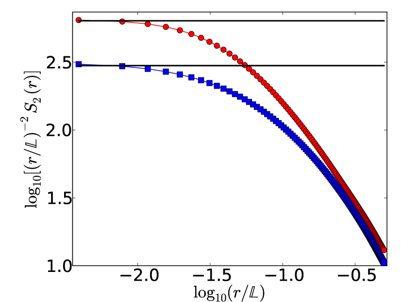
In Fig. 2 we give a log-log plot of $S_{2}(r)$, compensated by $(r/\mathbb{L})^{-2}$, as a function of $r/\mathbb{L}$. We find that, for small $r$, $S_{2}(r)\sim r^{2}$, which implies that our DNS resolves the analytic range, which follows from a Taylor expansion, of $S_{2}(r)$ sch+sre+yak89 ; this guarantees that energy-dissipation rate has been calculated accurately.

Figure 2: (Color online) Log-log (base 10) plots of the second-order structure function $S_{2}(r)$, compensated by $(r/\mathbb{L})^{-2}$, versus $r/\mathbb{L}$, for our run NSP-256B (blue square) and for the pure-fluid case (red circle). The regions in which the horizonal black lines overlap with the points indicate the $r^{2}$ scaling ranges.

In Fig. 3 we present plots of $\epsilon_{\nu}(t)$ versus $t/T_{\rm eddy}$ for $We=3.5$ and $We=7.1$ with the polymer concentration $c=0.1$. We find that the average value of $\epsilon_{\nu}$ decreases as we increase $We$.

Figure 3: (Color online) Plots of the energy dissipation rate $\epsilon_{\nu}$ versus $t/T_{\rm eddy}$ (runs NSP-256A and NSP-256B) for Weissenberg numbers $We=3.5$ (blue circles) and $We=7.1($black dashed line$)$. The corresponding plot for the pure fluid case is also shown for comparison (red line). The polymers are added to the fluid at $t=27T_{\rm eddy}$.

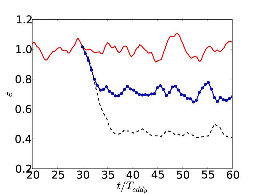
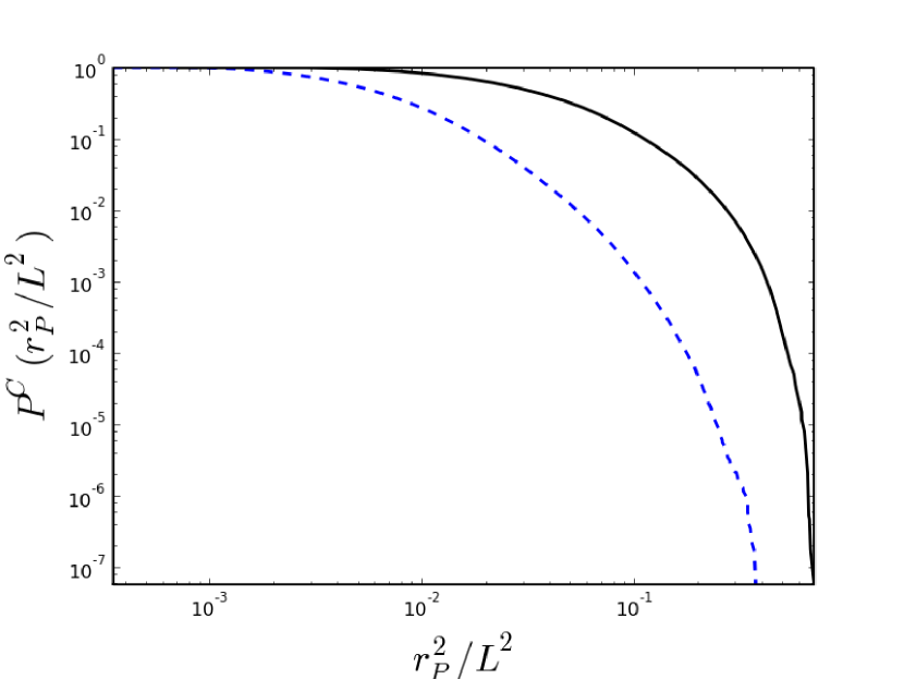
This suggests the following natural definition of the percentage dissipation reduction for forced, homogeneous, isotropic turbulence: here (and henceforth) the superscripts f and p stand, respectively, for the fluid without and with polymers; and the angular brackets denote an average over the statistically steady state. Percentage dissipation reduction, ${\rm DR}$, rises with $We$; this indicates that $\epsilon^{\rm p}_{\nu}$ increases with $We$. Thus, in contrast to the trend we observed in our decaying-turbulence DNS per06 , ${\rm DR}$ increases with $We$: For $We=3.5$, ${\rm DR\simeq 30\%}$ and, for $We=7.1$, ${\rm DR\simeq 50\%}$. Our interpretation is that this increase of ${\rm DR}$ with $We$ arises because the polymer extensions and, therefore, the polymer stresses are much stronger in our forced-turbulence DNS than in our decaying-turbulence DNS (at least for the Reynolds numbers that we achieved in Ref. per06 ). In Fig. 4 we show the cumulative PDF of the scaled polymer extension; this shows clearly that the extension of the polymers increases with $We$. In general, the calculation of PDFs from numerical data is plagued by errors originating from the binning of the data to make histograms. Here instead we have used the rank-order method to calculate the corresponding cumulative PDF which is free of binning errors mit05a .

Figure 4: (Color online) Log-log (base 10) plots of the cumulative PDF $P^{C}(r_{\rm P}^{2}/L^{2})$ versus the scaled polymer extension $r_{\rm P}^{2}/L^{2}$ for $We=3.5$ (blue dashed line for run NSP-256A) and $We=7.1$ (full black line for run NSP-256B). Note that as $We$ increases so does the extension of the polymers. These plots are obtained from polymer configurations at $t=60T_{\rm eddy}$.

III.2 Energy spectra

In this subsection we study fluid-energy spectra $E^{\rm p}(k)$, in the presence of polymer additives, for two different values of the Weissenberg number $We$ and fixed polymer concentration $c=0.1$ (Fig. 5). We find that the energy content at intermediate wave-vectors decreases with an increase in $We$. At small wave-vector magnitudes $k$, we observe a small increase in the spectrum on the addition of the polymers, but this increase is within our numerical, two-standard-deviation error bars. Because of the moderate resolution of our simulations we are not able to resolve the dissipation range fully in these simulations. We address this issue by conducting high-resolution, low-Reynolds-number simulations in Sec. III.4.

Figure 5: (Color online) Log-log plots (base 10) of the energy spectra $E^{\rm p}(k)$ versus $k$ (runs NSP-256A and NSP-256B) for $c=0.1$ and $We=3.5$ (blue squares) or $We=7.1$ (black stars); we give two-standard-deviation error bars. The corresponding pure-fluid spectrum $E^{\rm f}(k)$ (red circles) is shown for comparison.

III.3 Small-scale structures

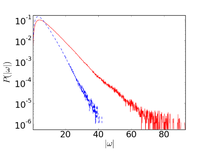
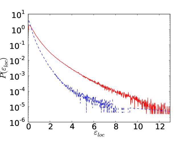
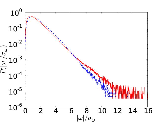
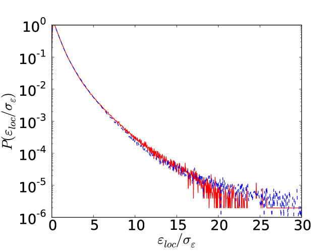
We now investigate how polymers affect small-scale structures in homogeneous, isotropic, fluid turbulence; and we make specific comparisons with experiments lib05 ; lib06 . We begin by plotting the PDFs of the modulus of the vorticity $|{\bm{\omega}}|$ and the local energy dissipation rate $\epsilon_{\rm loc}=\sum_{i,j}(\partial_{i}u_{j}+\partial_{j}u_{i})^{2}/2$ in Figs. 6. We find that the addition of polymers reduces regions of high vorticity and high dissipation [Figs. (6)]. Furthermore, we find that, on normalising $|{\bm{\omega}}|$ or $\epsilon_{\rm loc}$ by their respective standard deviations, the PDFs of these normalised quantities for the fluid with and without polymers collapse onto each other (within our numerical error bars) as shown in Figs. 7. Our results for these PDFs are in qualitative agreement with the results of Refs. lib05 ; lib06  (see Fig. $2$ of Ref. lib05 and Fig. $3$ of Ref. lib06 ).

Figure 6: (Color online) Semilog plots (base 10) of the PDFs $P(|{\bm{\omega}}|)$ versus $|{\bm{\omega}}|$ (top panel) and $P(\epsilon_{\rm loc})$ versus $\epsilon_{\rm loc}$ (bottom panel), for our run NSP-256B, with [$c=0.1$, $We=7.1$ (blue, dashed line)] and without [$c=0$ (full, red line)] polymer additives.

Figure 7: (Color online) Semilog plots (base 10) of the scaled PDFs $P(|{\bm{\omega}}|/\sigma)$ versus $|{\bm{\omega}}|/\sigma_{\omega}$ (top panel) and $P(\epsilon_{\rm loc}/\sigma_{\epsilon})$ versus $\epsilon_{\rm loc}/\sigma_{\epsilon}$ (bottom panel), where $\sigma_{\omega}$ and $\sigma_{\epsilon}$ are the standard deviations for $|{\bm{\omega}}|$ and $\epsilon_{\rm loc}$, respectively, for our run NSP-256B, with [$c=0.1$, $We=7.1$ (dashed line)] and without [$c=0$ (line)] polymer additives. These plots are normalized such that the area under each curve is unity.

Earlier high-resolution, large-$Re_{\lambda}$, DNS studies of homogeneous, isotropic fluid turbulence without polymer additives (see, e.g., Ref. kan03 ; per09b and references therein) have established that iso-$|{\bm{\omega}}|$ surfaces are filamentary for large values of $|{\bm{\omega}}|$. In Fig. III.3 we show how such iso-$|{\bm{\omega}}|$ surfaces change on the addition of polymers ($c=0.1$; $We=3.5$ or $7.1$). In particular, the addition of polymers suppresses a significant fraction of these filaments (compare the top and middle panels of Fig. III.3); and this suppression becomes stronger as $We$ increases (middle and bottom panels of Fig. III.3).

Figure 8: (Color online) Constant-$|{\bm{\omega}}|$ isosurfaces for $|{\bm{\omega}}|=\overline{|{\bm{\omega}}|}+2\sigma_{\omega}$ at $t\approx 60T_{\rm eddy}$ without (top panel) and with polymers [middle panel $We=3.5$ (NSP-256A) and bottom panel $We=7.1$ (run NSP-256B)]; $\overline{|{\bm{\omega}}|}$ is the mean and $\sigma_{\omega}$ the standard deviation of $|{\bm{\omega}}|$.

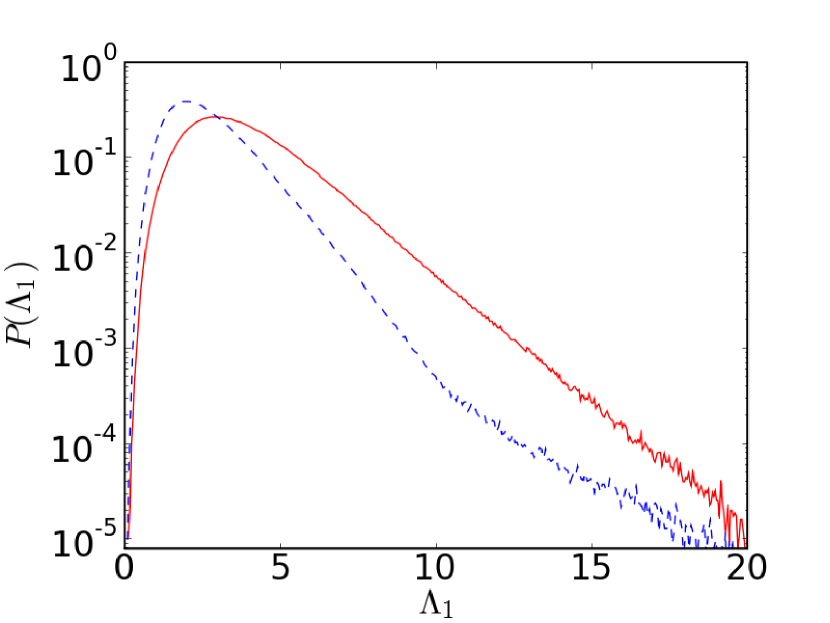
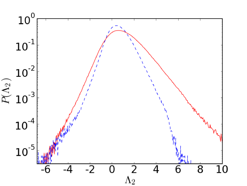
In addition to suppressing events which contribute to large fluctuations in the vorticity, the addition of polymers also affects the statistics of the eigenvalues of the rate-of-strain matrix ($S_{ij}=(\partial_{i}u_{j}+\partial_{j}u_{i})/\sqrt{2}$), namely, $\Lambda_{n}$, with $n=1,2,3$. They provide a measure of the local stretching and compression of the fluid. In our study, these eigenvalues are arranged in decreasing order, i.e., $\Lambda_{1}>\Lambda_{2}>\Lambda_{3}$. Incompressibility implies that $\sum_{i}\Lambda_{i}=0$; therefore, for an incompressible fluid, one of the eigenvalues ($\Lambda_{1}$) must be positive and one ($\Lambda_{3}$) negative. The intermediate eigenvalue $\Lambda_{2}$ can either be positive or negative. In Figs. (9) and (10) we plot the PDFs of these eigenvalues. The tails of these PDFs shrink on the addition of polymers. This indicates that the addition of the polymers leads to a substantial decrease in the regions where there is large strain, a result that is in qualitative agreement with the experiments of Ref. lib05 (see Fig. $3$(b) of Ref. lib05 ).

Figure 9: (Color online) Semilog (base 10) plots of the PDF $P(\Lambda_{1})$ versus the first eigenvalue $\Lambda_{1}$ of the strain-rate tensor $S$ for the run $\tt NSP-256B$, with [$We=7.1$ (blue dashed line)] and without [$c=0$ (full red line)] polymer additives. These plots are normalized such that the area under each curve is unity.

Figure 10: (Color online) Semilog (base 10) plots of the PDF $P(\Lambda_{2})$ versus the second eigenvalue $\Lambda_{2}$ of the strain-rate tensor $S$ for the run $\tt NSP-256B$, with [$We=7.1$ (blue dashed line)] and without [$c=0$ (full red line)] polymer additives. These plots are normalised such that the area under each curve is unity.

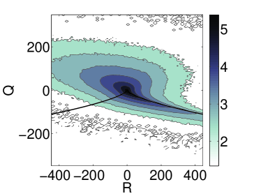
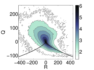
Evidence for the suppression of small-scale structures on the addition of polymers can also be obtained by examining the attendant change in the topological properties of a three-dimensional, turbulent flow. For incompressible, ideal fluids in three dimensions there are two topological invariants: $Q\equiv-{\rm Tr}(A^{2})/2$ and $R\equiv-{\rm Tr}(A^{3})/3$, where $A$ is the velocity-gradient tensor ${\nabla{\bf u}}$ . Topological properties of such a flow can be classified per+cho87 ; can92 by a $Q-R$ plot, which is a contour plot of the joint probability distribution function (PDF) of $Q$ and $R$. In Fig. 11 we give $Q-R$ plots from our DNS studies with and without polymers; although the qualitative shape of these joint PDFs remains the same, the regions of large $R$ and $Q$ are dramatically reduced on the additions of polymers; this is yet another indicator of the suppression of small-scale structures.

Figure 11: (Color online) Contour plots of the joint PDF $P(R,Q)$ from our DNS studies with (left) and without (right) polymer additives. In this $Q-R$ plot, $Q=-{\rm Tr}(A^{2})/2$ and $R=-{\rm Tr}(A^{3})/3$ are the invariants of the velocity-gradient tensor ${\nabla{\bf u}}$. Note that $P(R,Q)$ shrinks on the addition of polymers; this indicates a depletion of small-scale structures. The contour levels are logarithmically spaced and are drawn at the following values: $1.3,2.02,2.69,3.36,4.04,4.70,5.38$, and $6.05$.

III.4 Effects of polymer additives on deep-dissipation-range spectra

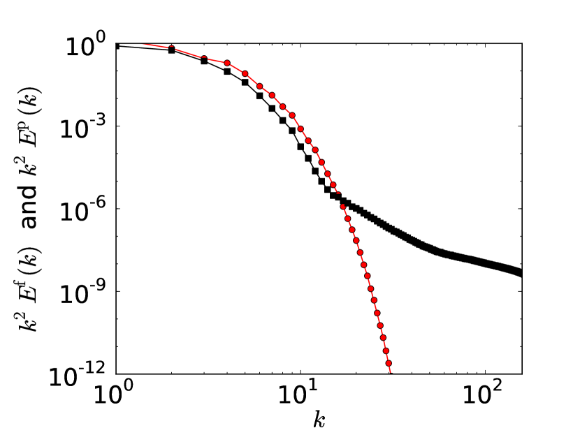
In the previous subsections we have studied the effects of polymer additives on the structural properties of a turbulent fluid at moderate Reynolds numbers. We now investigate the effects of polymer additives on the deep-dissipation range. To uncover such deep-dissipation-range effects, we conduct a very high-resolution, but low-$Re_{\lambda}$ ($=16$) DNS study (${\tt NSP-512}$). The parameters used in our run ${\tt NSP-512}$ are given in Table 1. The fluid is driven by using the stochastic-forcing scheme of Ref. esw88 . In Fig. 12 we plot fluid-energy spectra with and without polymer additives. The general behavior of these energy spectra is similar to that in our decaying-turbulence study per06 . We find that, on the addition of polymers, the energy content at intermediate wave-vectors decreases, whereas the energy content at large wave-vectors increases significantly. We have checked explicitly that this increase in the energy spectrum in the deep-dissipation range is not an artifact of aliasing errors: Note first that this increase starts at wave vectors whose magnitude is considerably lower than the dealiasing cutoff $k_{\rm max}$ in our DNS; furthermore, the enstrophy spectrum $k^{2}E^{\rm p}(k)$, which we plot versus $k$ in Fig. 13, decays at large $k$; this indicates that the dissipation range has been resolved adequately in our DNS.

Figure 12: (Color online) Log-log (base 10) plots of the fluid-energy spectrum $E^{\rm p}(k)$ versus the magnitude of the wave vector $k$ for our run ${\tt NSP=512}$ (full black line with squares) for $c=0.1$ and $\tau_{\rm P}=1$. The corresponding plot for the pure fluid (full red line with circles) is also shown for comparison.

Figure 13: (Color online) Log-log (base 10) plots of the enstrophy spectrum $k^{2}E^{\rm p}(k)$ versus the magnitude of the wave vector $k$ for our run ${\tt NSP=512}$ (full black line with squares) for $c=0.1$ and $\tau_{\rm P}=1$. The corresponding plot for the pure fluid (full red line with circles) is also shown for comparison.

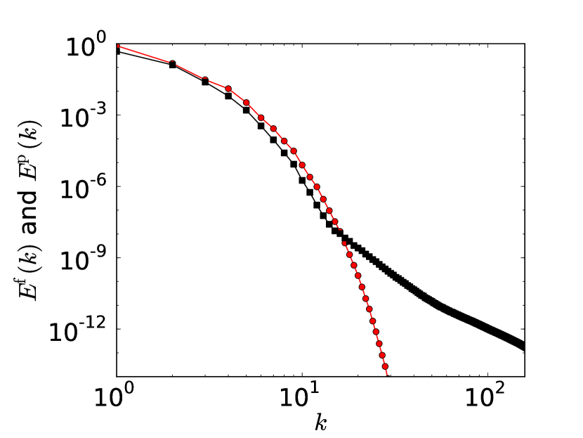
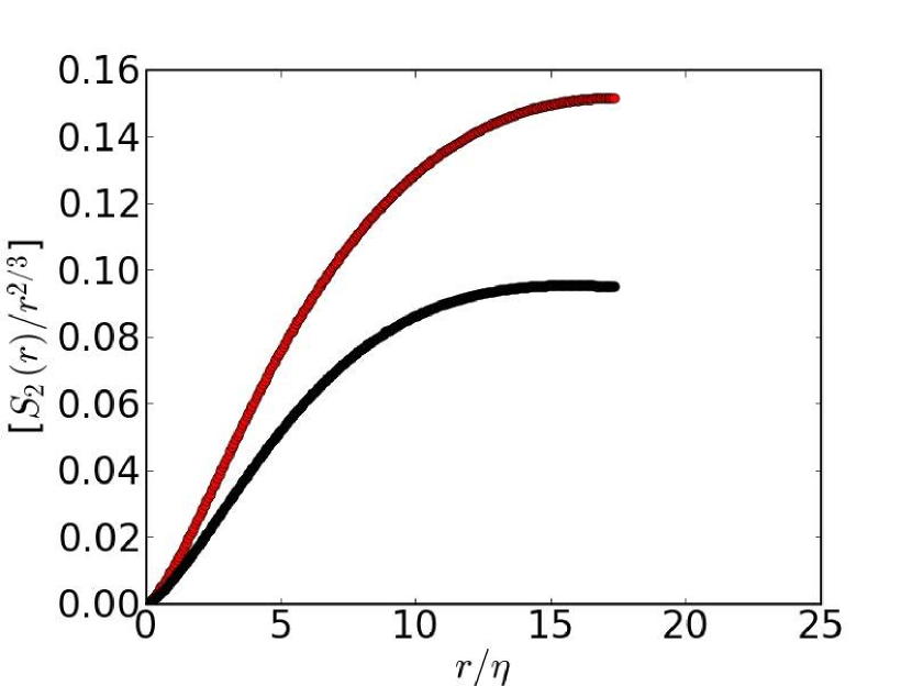
For homogeneous, isotropic turbulence, the relationship between the second-order structure function and the energy spectrum is given in Eq. (10) Bat53 . Using this relationship and the data for the energy spectrum shown in Fig. 12, we have obtained the second-order structure function $S_{2}(r)$ for our run ${\tt NSP-512}$. We find that the addition of polymers leads to a decrease in the magnitude of $S_{2}(r)$. Our plots for $S_{2}(r)$ are similar to those found in the experiments of Ref. oue09 . In our simulations we are able to reach much smaller values of $r/\eta$ than has been possible in experimental studies on these systems oue09 ; however, we have not resolved the inertial range very well in these runs. Note that the spectra $E^{\rm p}(k)$, with polymers, and $E^{\rm f}(k)$, without polymers, cross each other as shown in Fig. 12. But such a crossing is not observed in the corresponding plots of second-order structure functions (Fig. 14). This can be understood by noting that $S_{2}(r)$ combines large- and small-$k$ parts Dav04 of the energy spectrum.

Figure 14: (Color online) Plots of the compensated second-order structure function $S_{2}(r)/r^{2/3}$ versus $r/\eta$ with (black circles) and without (red circles) polymer additives for our run ${\tt NSP-512}$.

IV Conclusions

We have presented an extensive numerical study of the effects of polymer additives on statistically steady, homogeneous, isotropic fluid turbulence. Our study complements, and extends considerably, our earlier work per06 . Furthermore, our results compare favorably with several recent experiments.

Our first set of results show that the average viscous energy dissipation rate decreases on the addition of polymers. This allows us to extend the definition of dissipation reduction, introduced in Ref. per06 , to the case of statistically steady, homogeneous, isotropic, fluid turbulence with polymers. We find that this dissipation reduction increases with an increase in the Weissenberg number $We$, at fixed polymer concentration $c$. We obtain PDFs of the modulus of the vorticity, of the eigenvalues $\Lambda_{n}$ of the rate-of-strain tensor $S$, and $Q-R$ plots; we find that these are in qualitative agreement with the experiments of Refs. lib05 ; lib06 .

Our second set of results deal with a high-resolution DNS that we have carried out to elucidate the deep-dissipation-range forms of (a) energy spectra and (b) the related second-order velocity structure functions. We find that this deep-dissipation-range behavior is akin to that in our earlier DNS of decaying, homogeneous, isotropic, fluid turbulence with polymers per06 . Furthermore, the results we obtain for the scaled, second-order, velocity structure $S_{2}(r)$ yield trends that are in qualitative agreement with the experiments of Ref. oue09 .

We hope that the comprehensive study that we have presented here will stimulate further detailed experimental studies of the statistical properties of homogeneous, isotropic fluid turbulence with polymer additives.

V Acknowledgments

We thank J. Bec, E. Bodenschatz, F. Toschi, and H. Xu for discussions, Leverhume trust, European Research Council under the AstroDyn Research Project No. 227952, CSIR, DST, and UGC (India) for support, and SERC (IISc) for computational resources. Two of us (RP and PP) are members of the International Collaboration for Turbulence Research and they acknowledge support from the COST Action MP0806. While most of this work is being carried out PP was a student at IISc.

References

- (1) J. Hoyt and J. Taylor, Phys. Fluids. 20, S253 (1977).
- (2) C. Kalelkar, R. Govindarajan, and R. Pandit, Phys. Rev. E 72, 017301 (2004).
- (3) P. Perlekar, D. Mitra, and R. Pandit, Phys. Rev. Lett. 97, 264501 (2006).
- (4) B. Toms, in Proceedings of First International Congress on Rheology (North-Holland, Amsterdam, 1949), pp. Section II, 135.
- (5) J. Lumley, J. Polymer Sci 7, 263 (1973).
- (6) P. Virk, AIChE 21, 625 (1975).
- (7) J.M.J. Den Toonder, M.A. Hulsen, G.D.C. Kuiken and F. Nieuwstadt, J. Fluid. Mech. 337, 193 (1997).
- (8) Y. Dubief and S. Lele, Annual research briefs, Center for Turbulence Research (unpublished).
- (9) P. Ptasinski, F. Nieuwstadt, B. V. den Brule, and M. Hulsen, Flows, Turbulence and Combustion 66, 159 (2001).
- (10) P. Ptasinski et al., J. Fluid. Mech 490, 251 (2003).
- (11) V. L’vov, A. Pomyalov, I. Procaccia, and V. Tiberkevich, Phys. Rev. Lett. 92, 244503 (2004).
- (12) E. De Angelis, C. Casicola, R. Benzi, and R. Piva, J. Fluid. Mech 531, 1 (2005).
- (13) I. Procaccia, V. Ĺvov, and R. Benzi, Rev. Mod. Phys. 80, 225 (2008).
- (14) N. Ouellette, H. Xu, and E. Bodenschatz, J. Fluid Mech. 629, 375 (2009). A.M Crawford, N. Mordant, H. Xu and E. Bodenschatz, New Journal of Physics 10 (2008) 123015. A.M Crawford, N. Mordant, A.La Porta and E. Bodenschatz, in Advances in Turbulence IX, Ninth European Turbulence Conference, I.P. Castro, P.E. Hancock and T.G. Thomas (Eds), CIMNE, Barcelona, 2002.
- (15) A. Liberzon et al., Phys. Fluids. 17, 031707 (2005).
- (16) A. Liberzon, M. Guala, W. Kinzelbach, and A. Tsinober, Phys. Fluids. 18, 125101 (2006).
- (17) R. Benzi, E. De Angelis, R. Govindarajan, and I. Procaccia, Phys. Rev. E 68, 016308 (2003).
- (18) T. Vaithianathan and L. Collins, Journal of Computational Physics 187, 1 (2003).
- (19) A. Lamorgese, D. Caughey, and S. Pope, Phys. Fluids 17, 015106 (2005).
- (20) V. Eswaran and S. Pope, Computers and Fluids 16, 257 (1988).
- (21) C. Canuto, M. Hussaini, A. Quarteroni, and T. Zang, Spectral methods in Fluid Dynamics (Spinger-Verlag, Berlin, 1988).
- (22) A. Vincent and M. Meneguzzi, J. Fluid. Mech. 225, 1 (1991).
- (23) T. Vaithianathann, A. Robert, J. Brasseur, and L. Collins, J. Non-newtonian Fluid Mech. 140, 3 (2006).
- (24) A. Kurganov and E. Tadmor, J. Comp. Phys. 160, 241 (2000).
- (25) G. Batchelor, The theory of homogeneous turbulence (Cambridge University Press, Cambridge, 1953).
- (26) J. Schumacher, K.R. Sreenivasan and V. Yakhot, New J. Phys., 9, 89 (2007).
- (27) A. Robert, T. Vaithianathan, L. Collins, and J. Brasseur, Journal of Fluid Mechanics, in press, (2010).
- (28) D. Mitra, J. Bec, R. Pandit, and U. Frisch, Phys. Rev. Lett 94, 194501 (2005).
- (29) Y. Kaneda et al., Physics of Fluids 15, L21 (2003).
- (30) R. Pandit, P. Perlekar, and S.S. Ray, Pramana 73, 179 (2009).
- (31) A. Perry and M. Chong, Annu. Rev. Flu. Mech. 19, 125 (1987).
- (32) B. Cantwell, Phys. Fluids A 4, 782 (1992).
- (33) P. Davidson, Turbulence (Oxford University Press, New York, 2004), pp. 386–410.