Acoustic metafluids made from three acoustic fluids

Abstract

Significant reduction in target strength and radiation signature can be achieved by surrounding an object with multiple concentric layers comprised of three acoustic fluids. The idea is to make a finely layered shell with the thickness of each layer defined by a unique transformation rule. The shell has the effect of steering incident acoustic energy around the structure, and conversely, reducing the radiation strength. The overall effectiveness and the precise form of the layering depends upon the densities and compressibilities of the three fluids. Nearly optimal results are obtained if one fluid has density equal to the background fluid, while the other two densities are much greater and much less than the background values. Optimal choices for the compressibilities are also found. Simulations in 2D and 3D illustrate effectiveness of the three fluid shell. The limited range of acoustic metafluids that are possible using only two fluid constituents is also discussed.

1 Introduction

The idea behind transformation acoustics is that a coordinate transformation makes it possible to have one region of an acoustic fluid mimic another region. Fluids that have this property have been called acoustic metafluids. In transformation optics the transformation uniquely defines the material properties, but this is not the case in acoustics, and there is an added degree of freedom in the makeup of the acoustic metafluid. The range of possible acoustic metafluids has been derived Norris (2009), and includes fluids with anisotropic inertia and pentamode materials.

Interest in transformation acoustics has been motivated by the possibility of acoustic cloaking. The first electromagnetic wave cloaking device Pendry et al. (2006) uses transformation of coordinates in the governing wave equation to steer energy around the cloaked object. It was subsequently demonstrated that the same methods should work for the acoustic wave equation Cummer and Schurig (2007); Chen and Chan (2007). The acoustic cloak corresponds to the limiting case of a point transformed into a finite region, and it has unavoidable physical singularities associated with the extreme nature of the transformation. Different types of singularities are obtained depending on whether the transformed metafluid is purely inertial with anisotropic density and a single bulk modulus, or in the other limit, purely pentamodal with isotropic inertia. The distinction is important for cloaking, for which it is known that use of only fluids with anisotropic inertia (inertial cloaks) requires infinite mass, and is therefore not a realistic path towards acoustic cloaking Norris (2008). Despite this limitation, it is possible to achieve almost perfect, or near-cloaking, using layers of anisotropic fluids that approximate the transformed medium, without the singularity. For instance, Torrent and Sánchez-Dehesa Torrent and Sánchez-Dehesa (2008) partition the shell into many small but equally thin layers where the local properties are defined by two normal fluids, with density and bulk moduli $\{\rho_{j},K_{j}\}$, $j=1,2$, such that the averaged quantities $\rho_{r}=\frac{1}{2}(\rho_{1}+\rho_{2})$, $\rho_{\perp}=[\frac{1}{2}(\rho_{1}^{-1}+\rho_{2}^{-1})]^{-1}$ and $K=[\frac{1}{2}(K_{1}^{-1}+K_{2}^{-1})]^{-1}$ yield the anisotropic metafluid properties $\{\rho_{r}(r),\rho_{\perp}(r),K(r)\}$ proposed by Cummer and Schurig Cummer and Schurig (2007). In order to achieve this equivalence it is necessary to make $\{\rho_{j},K_{j}\}$, $j=1,2$, functions of $r$, with the result a large number of distinct fluids is necessary: 100 and 400 for the two numerical examples reported by Torrent and Sánchez-Dehesa Torrent and Sánchez-Dehesa (2008).

The purpose of this paper is to demonstrate that significant reduction in target strength can be achieved using layers comprised of only three acoustic fluids. The idea is to make a finely layered shell that surrounds the structure, with each layer being one of the three fluids, but instead of prescribing the relative thickness of each layer we allow it to be a function of $r$. The transformation formulas then imply unique values for the relative concentrations as functions of $r$, in both two (cylinder) and three (sphere) dimensions.

The outline of the paper is as follows. The homogenized layered shell and the transformation metamaterial are introduced separately in Section 2 in the context of an $N-$fluid material. The remainder of the paper concentrates on the 3-fluid $(N=3)$ configuration. General results for both cylindrical and spherical shells are derived in Section 3, including the unique transformation formulae. Dependence of the cylindrical transformation metamaterial on the constituent properties of the 3-fluids is explored in Section 4. The explicit nature of the transformation formulae for 2D suggest optimal choices for the fluid densities and compressibilities. These findings are confirmed in Section 5 where examples of cylindrical and spherical 3-fluid metamaterials are presented. Numerical simulations showing their effectiveness in reducing scattering strength in 2 and 3 dimensions are also presented in Section 5.

2 Preliminaries

We consider radially symmetric configurations, cylindrical in 2D and spherical in 3D. A fluid annulus or shell occupies $0<r_{0}\leq r\leq r_{out}$, and is surrounded by a uniform acoustic medium with density and sound speed $\rho_{out}$, $c_{out}$, in $r>r_{out}$. The shell is assumed to be made of a finite number, $N$, of distinct fluids arranged in a well defined stratification that results in an effective material with smoothly varying properties in the radial direction. We are particularly interested in finding the smallest number $N$ for which it is possible that the stratification has the properties of an acoustic metafluid. An acoustic metafluid is defined here as a material with desirable effective properties that cannot easily be obtained with a single, physical fluid. This definition obviously includes materials obtained by a coordinate transformation of a larger region of uniform acoustic fluid with properties equal to those of the exterior fluid in $r>r_{out}$.

For simplicity, but with no lack in generality, we set $r_{out}=1$, $c_{out}=1$ and $\rho_{out}=1$, which is equivalent to choosing units for length, time and mass, respectively. For the remainder of the paper all quantities are non-dimensional.

We first consider the homogenized shell composed of a layering of $N$ distinct fluids defined by their mass densities, $\rho_{1},\ldots,\rho_{N}$, and the compressibilities $C_{1},\ldots,C_{N}$. The compressibility is $C_{i}=K_{i}^{-1}$ where $K_{i}$ is the bulk modulus, and the wave speeds are $c_{i}=\sqrt{K_{i}/\rho_{i}}$, and the impedances are $z_{i}=\sqrt{K_{i}\rho_{i}}$, $i=1,\ldots,N$. We define, for later use, $S_{i}=\rho_{i}C_{i}$, or alternatively, $S_{i}=c_{i}^{-2}$, so that we may identify $\sqrt{S_{i}}$ as acoustic slowness in fluid $i$.

The layering yields an effective fluid with compressibility $C_{*}$ and anisotropic inertia defined by radial density $\rho_{r}$, and circumferential density $\rho_{\perp}$. The parameters of the effective fluid are defined by homogenization of the stratified medium as Schoenberg and Sen (1983)

$$\begin{pmatrix}\rho_{r}\\ \rho_{\perp}^{-1}\\ C_{*}\end{pmatrix}=\begin{pmatrix}\langle\rho\rangle\\ \langle\rho^{-1}\rangle\\ \langle C\rangle\end{pmatrix},$$ (1)

where $\langle\cdot\rangle$ is the local average over the volume fractions of the $N$-fluids,

$$\langle x\rangle=\sum_{i=1}^{N}\phi_{i}x_{i},\quad\text{with }\langle 1\rangle=1.$$ (2)

It is assumed that $\phi_{i}=\phi_{i}(r)$, so that the averages (1) define parameters $\rho_{r}(r)$, $\rho_{\perp}(r)$, and $C_{*}(r)$. This type of inhomogeneous or localized homogenization may be achieved by allowing the layering to be sufficiently fine, and will be illustrated by numerical examples later.

The transformation from the current (physical) domain to the mimicked one makes the shell appear acoustically as if it is a larger shell of fluid with uniform properties equal to the exterior fluid. The key is a transformation function, $r\rightarrow R=R(r)$, such that the range of $R$ exceeds its domain, i.e., the inverse mapping $R\rightarrow r$ physically contracts space. To be specific, the outer boundary is mapped to itself, $r=R=1$, and the inner boundary $r=r_{0}$ is mapped to $R=R_{0}$, with $0<R_{0}=R(r_{0})<r_{0}$. The perfect acoustic cloak is defined by $R_{0}=0$. The transformed material has properties $\rho_{rT}$, $\rho_{\perp T}$, and $C_{*T}$, with values uniquely defined by the transformation in $d-$dimensions as Norris (2008)

$$\begin{pmatrix}\rho_{rT}\\ \rho_{\perp T}^{-1}\\ C_{*T}\end{pmatrix}=R^{\prime}\begin{pmatrix}(r/R)^{d-1}\\ (r/R)^{3-d}\\ (r/R)^{1-d}\end{pmatrix},\quad d=2\text{ or }3,$$ (3)

and where $R^{\prime}=\operatorname{d}R/\operatorname{d}r$.

The connection between the homogenized material (1) and the acoustically transformed material (3) is now made explicit by requiring $\rho_{rT}=\rho_{r}$, $\rho_{\perp T}=\rho_{\perp}$ and $C_{*T}=C_{*}$ (and we drop the subscript $T$). Our objective is to find families of transformation functions $R=R(r)$, $\phi_{i}=\phi_{i}(r)$ for which this equivalence can be achieved. It depends, of course, on the choices of material properties $\{\rho_{i},C_{i}\}$, $i=1,\ldots,N$, and not all combinations will work. Among the requirements are that the transformation function is one-to-one, and that the volume fractions are all between zero and unity. We therefore require that ${\boldsymbol{\phi}}\in\Phi_{N}$ where ${\boldsymbol{\phi}}$ is the $N-$dimensional vector of volume fractions, and $\Phi_{N}$ the $N-1$ dimensional surface on which it must lie,

$$\Phi_{N}=\{\phi_{i}\geq 0,\,\,\sum_{i}\phi_{i}=1,\,\,i=1,\ldots,N\}.$$ (4)

3 The three fluid material

3.1 Algebraic formulation

The first two relations in (1) and the identity $\eqref{-54}_{2}$ may be written in matrix form for $N=3$,

$$\begin{pmatrix}1&1&1\\ \rho_{1}&\rho_{2}&\rho_{3}\\ {\rho_{1}^{-1}}&{\rho_{2}^{-1}}&{\rho_{3}^{-1}}\end{pmatrix}\begin{pmatrix}\phi_{1}\\ \phi_{2}\\ \phi_{3}\end{pmatrix}=\begin{pmatrix}1\\ \rho_{r}\\ \rho_{\perp}^{-1}\end{pmatrix}.$$ (5)

This can be solved to give the 3-vector of volume fractions in terms of $\rho_{r}$ and $\rho_{\perp}^{-1}$. Substitution into the third relation in (1) yields an expression for $C_{*}$ in terms of $\rho_{r}$ and $\rho_{\perp}^{-1}$. Thus,

$${\boldsymbol{\phi}} ={\boldsymbol{f}}_{0}+\rho_{r}{\boldsymbol{f}}_{1}+\rho_{\perp}^{-1}{\boldsymbol{f}}_{2},$$ (6a)

$$C_{*} =\alpha+\beta_{1}\rho_{r}+\beta_{2}\rho_{\perp}^{-1},$$ (6b)

where the 3-vectors in (6a) are

$${\boldsymbol{\phi}} =\begin{pmatrix}\phi_{1}\\ \phi_{2}\\ \phi_{3}\end{pmatrix}, {\boldsymbol{f}}_{0}=D\begin{pmatrix}\frac{\rho_{2}}{\rho_{3}}-\frac{\rho_{3}}{\rho_{2}}\\ \frac{\rho_{3}}{\rho_{1}}-\frac{\rho_{1}}{\rho_{3}}\\ \frac{\rho_{1}}{\rho_{2}}-\frac{\rho_{2}}{\rho_{1}}\end{pmatrix},$$

$${\boldsymbol{f}}_{1} =D\begin{pmatrix}\frac{1}{\rho_{2}}-\frac{1}{\rho_{3}}\\ \frac{1}{\rho_{3}}-\frac{1}{\rho_{1}}\\ \frac{1}{\rho_{1}}-\frac{1}{\rho_{2}}\end{pmatrix}, {\boldsymbol{f}}_{2}=D\begin{pmatrix}\rho_{3}-\rho_{2}\\ \rho_{1}-\rho_{3}\\ \rho_{2}-\rho_{1}\end{pmatrix},$$ (7)

with $D={\rho_{1}\rho_{2}\rho_{3}}/[(\rho_{1}-\rho_{2})(\rho_{2}-\rho_{3})(\rho_{3}-\rho_{1})]$, and the scalars $\alpha$, $\beta_{1}$ and $\beta_{2}$ in (6b) are

$$\quad\alpha={\boldsymbol{C}}^{T}{\boldsymbol{f}}_{0},\quad\beta_{1}={\boldsymbol{C}}^{T}{\boldsymbol{f}}_{1},\quad\beta_{2}={\boldsymbol{C}}^{T}{\boldsymbol{f}}_{2},$$ (8)

with ${\boldsymbol{C}}^{T}=(C_{1},C_{2},C_{3})$.

3.2 The transformation function

3.2.1 Differential equations

Eliminating $C_{*}$, $\rho_{r}$ and $\rho_{\perp}^{-1}$ from (6b) using the identities (3) yields a differential equation for the transformation function,

$$\frac{\operatorname{d}R}{\operatorname{d}r}=\begin{cases}\alpha\big{(}\frac{R}{r}-\beta\frac{r}{R}\big{)}^{-1},&2D,\\ &\\ \alpha\big{(}\frac{R^{2}}{r^{2}}-\beta_{1}\frac{r^{2}}{R^{2}}-\beta_{2}\big{)}^{-1},&3D,\end{cases}$$ (9)

subject to the boundary condition $R(1)=1$. The parameters $\beta$ and, for later use, $\lambda$, $\mu$, are defined

$$\beta=\beta_{1}+\beta_{2},\quad\lambda=\alpha+\beta,\quad\mu=-\frac{\beta}{\alpha}.$$ (10)

3.2.2 2D solution

We first consider the 2D equation $\eqref{0345}_{1}$. Let $x=r^{2}$, $X=R^{2}$, then eq. $\eqref{0345}_{1}$ becomes

$$X\frac{\operatorname{d}x}{\operatorname{d}X}+\frac{\beta}{\alpha}x=\frac{X}{\alpha},\qquad x(1)=1.$$ (11)

Integrating yields

$$r=\bigg{(}\frac{R^{2}+(\lambda-1)R^{2\mu}}{\lambda}\bigg{)}^{1/2}.$$ (12)

The 2D transformation function is therefore completely defined by the two parameters $\lambda$ and $\mu$, given in explicit form in (A.1).

3.2.3 3D solution

The 3D equation $\eqref{0345}_{2}$ becomes, with the change of variable $s=\frac{r}{R}$,

$$\frac{1}{R}\frac{\operatorname{d}R}{\operatorname{d}s} =\frac{-\alpha s^{2}}{\beta_{1}s^{4}+\alpha s^{3}+\beta_{2}s^{2}-1}$$

$$=\sum_{i=1}^{4}\frac{\gamma_{i}}{s-s_{i}},\quad R(1)=1.,$$ (13)

where the four roots $s_{i}$ and the coefficients $\gamma_{i}$, $i=1,2,3,4$, are defined by

$$\beta_{1}\prod\limits_{j=1}^{4}(s-s_{j}) =\beta_{1}s^{4}+\alpha s^{3}+\beta_{2}s^{2}-1,$$ (14a)

$$\gamma_{i} =\frac{-\alpha s_{i}^{2}}{\beta_{1}\prod\limits_{j\neq i}(s_{i}-s_{j})}.$$ (14b)

Note that $\sum_{i}\gamma_{i}=0$, $\sum_{i}s_{i}=-\alpha/\beta_{1}$, $\sum_{i}\gamma_{i}s_{i}=-\alpha/\beta_{1}$, $\sum_{i}\gamma_{i}s_{i}^{2}=(\alpha/\beta_{1})^{2}$. Integration of (3.2.3) yields

$$R=\prod\limits_{i=1}^{4}\bigg{(}\frac{\frac{r}{R}-s_{i}}{1-s_{i}}\bigg{)}^{\gamma_{i}}.$$ (15)

This provides an implicit formula for $R$ and $r$, in terms of the three parameters $\alpha$, $\beta_{1}$ and $\beta_{2}$. Using the fact that $1\leq s\leq s_{0}$, where $s_{0}$ is defined in the next subsection, eq. (15) gives $R$ as a function of $s$, from which $r=sR$ is obtained.

Figure 1: The range of ${\boldsymbol{\phi}}$ for the 3-fluid.

3.3 The inner radii $r_{0}$ and $R_{0}$

It follows from continuity of the solution of the differential equation (9) that the values of the inner radii $r_{0}$ and $R_{0}$ should correspond to a point on the edge of the triangular region $\Phi_{3}$, see Fig. 1. The actual radial values can be determined from eq. (5), using $\rho_{r}$ and $\rho_{\perp}$ as defined in (3) and keeping the parameter $s=\frac{r}{R}$ to express $\phi_{i}$ of (6a) in the form

$$\phi_{i}=\frac{\rho_{i}\big{[}(s^{d-1}+\rho_{j}\rho_{k}s^{3-d})R^{\prime}-(\rho_{j}+\rho_{k})\big{]}}{(\rho_{i}-\rho_{j})(\rho_{i}-\rho_{k})},$$ (16)

where $i\neq j\neq k\neq i$. Replacing $R^{\prime}$ by (9) and setting (16) to zero implies an algebraic (polynomial) equation for $s$. In principle there are three possible solutions, corresponding to each of $\phi_{i}=0$, $i=1,2,3$. However, in practice for a given set of 3-fluids only one is important, and we choose the 3-fluid properties so that it is the root for $\phi_{2}=0$. We consider first $d=2$.

In the 2D cylindrical configuration the equation $\phi_{2}=0$ is a quadratic in $s$ with a single positive root greater than unity (corresponding to $r_{0}>R_{0}$), which combined with (12) implies $R_{0}$ and $r_{0}$ in explicit form as

$$R_{0} =\bigg{[}(\lambda-1)\bigg{(}\frac{\rho_{r2}^{-1}-\mu}{1-\rho_{r2}^{-1}}\bigg{)}\bigg{]}^{\frac{1}{2(1-\mu)}},$$ (17a)

$$r_{0} =\bigg{[}\lambda\bigg{(}\frac{\rho_{r2}^{-1}-\mu}{1-\mu}\bigg{)}\bigg{]}^{-\frac{1}{2}}R_{0},$$ (17b)

where

$$\rho_{ri}=\frac{\rho_{j}+\rho_{k}}{1+\rho_{j}\rho_{k}}\quad(i\neq j\neq k\neq i).$$ (18)

For the 3D spherical case the equation $\phi_{2}=0$ becomes a biquadratic in $s$. We find

$$R_{0}=\prod\limits_{i=1}^{4}\bigg{(}\frac{s_{0}-s_{i}}{1-s_{i}}\bigg{)}^{\gamma_{i}},\quad r_{0}=s_{0}R_{0},$$ (19)

where $s_{0}$ is a positive root of

$$s^{4}[\alpha+\beta_{1}(\rho_{1}+\rho_{3})]+s^{2}[\alpha\rho_{1}\rho_{3}+\beta_{2}(\rho_{1}+\rho_{3})]-(\rho_{1}+\rho_{3})=0.$$ (20)

The transformation requires $s_{0}>1$, and numerical experiments (see Section 5) indicate that a single real root greater than unity exists in all the cases considered.

3.4 Total mass and average density

The total mass $m$ of the 3-fluid shell is the integral of the local average of the density, $\langle\rho\rangle$. Therefore, $m$ follows from eq. (1) as the volumetric integral of $\rho_{r}(r)$. Substituting from (3)₁ and using (9), the integral can be expressed in closed form for the 2D case, and reduced to an integral in $s=r/R$ for the 3D case. We find

$$m=\begin{cases}\frac{\pi}{\lambda}\big{\{}1-R_{0}^{2}+\frac{(\lambda-1)}{\mu}\big{(}1-R_{0}^{2\mu}\big{)}\big{\}},&2D,\\ 4\pi\frac{\alpha}{\beta_{1}}\int\limits_{1}^{s_{0}}\,s^{6}\prod\limits_{i=1}^{4}\frac{\big{(}s-s_{i}\big{)}^{3\gamma_{i}-1}}{\big{(}1-s_{i}\big{)}^{3\gamma_{i}}}\operatorname{d}s,&3D,\end{cases}$$ (21)

from which the average density in the shell, $\bar{\rho}=3m/[\pi(d+1)(1-r_{0}^{d})]$, can be found. For 2D we find, after some simplification,

$$\bar{\rho}=\frac{1}{\mu}+\frac{1}{\beta}\bigg{(}\frac{1-R_{0}^{2}}{1-r_{0}^{2}}\bigg{)},\quad 2D.$$ (22)

3.5 Summary

We have shown that the three fluid shell is uniquely related to possible transformation functions in both 2- and 3-dimensions. The connection is still somewhat tentative, since we must confirm that the functions are physically realistic. This requires among other things that the volume fractions are all positive and between zero and unity, i.e. that ${\boldsymbol{\phi}}\in\Phi_{3}$ where the equilateral triangle surface $\Phi_{3}$ is defined by (4). We must also confirm that the inner radii are actually given by eqs. (17) in 2D and (19) in 3D. Optimally, both of the inner radii should be small, since $R_{0}\ll 1$ means that the mapped region $R_{0}\leq R\leq 1$ is almost the entire interior of the cylinder/sphere of radius $1$, while $R_{0}\ll r_{0}$ implies that the shell $r_{0}\leq r\leq 1$ in physical space occupies a relatively small proportion of the mapped region. In the next Section we consider the 2D shell for which these questions can be answered in explicit form.

The results for the 3-fluid shell indicate that there are no free parameters for a given set of fluids. This suggests that the transformation property cannot be achieved with only two fluids. It is shown in Appendix B that the 2-fluid case is too constrained, although it does display some interesting physical properties, even if it cannot provide acoustic cloaking.

4 The three fluid material in $2D$

4.1 Range of material parameters

The relation $\rho_{r}\rho_{\perp}=1$, which holds only in 2D (see eq. (3)), considerably simplifies the algebra of the problem as compared with the 3D case, allowing clearer understanding of parametric dependence. We refer the reader to Appendix A for the details and provide only the main findings here.

With no loss in generality, see Appendix A, we assume

$$\rho_{1}>\rho_{2}>\rho_{3},\text{ with }\quad\rho_{1}>1,\quad\rho_{3}<1.$$ (23)

The density with the intermediate value, $\rho_{2}$, may be less than, equal to, or greater than unity. In order to distinguish these two cases without being specific as to the particular one, we define $\rho_{p}$ as the density with value on the same side of unity as $\rho_{2}$. We assume for the moment that $\rho_{2}\neq 1$; the special case of $\rho_{2}=1$ is discussed separately below.

The main result is that the physically obtainable material properties can be parameterized in terms of the radial density $\rho_{r}$, which has a well defined range itself. Thus, ${\boldsymbol{\phi}}\in\Phi_{3}$ for $\rho_{rp}\leq\rho_{r}\leq\rho_{r2}$, where $\rho_{ri}$ are defined in (18). The lower bound is not achieved in practice but is instead set by the value of $\rho_{r}$ at $r=1$, see Appendix A. The physically reachable values of the volume fractions, compressibility and density $\rho_{\perp}$ are therefore defined through $\rho_{r}$ as

$${\boldsymbol{\phi}} ={\boldsymbol{\phi}}_{rp}+\big{(}\frac{\rho_{r}-\rho_{rp}}{\rho_{r2}-\rho_{rp}}\big{)}({\boldsymbol{\phi}}_{r2}-{\boldsymbol{\phi}}_{rp}),$$ (24a)

$$C_{*} =C_{*p}+\big{(}\frac{\rho_{r}-\rho_{rp}}{\rho_{r2}-\rho_{rp}}\big{)}(C_{*2}-C_{*p}),$$ (24b)

$$\rho_{\perp} =\rho_{r}^{-1},\quad\text{ for }\frac{\alpha}{1-\beta}\leq\rho_{r}\leq\rho_{r2},$$ (24c)

where the critical values $\rho_{ri}$ of the radial density are defined in (18), and the critical values of the concentrations ${\boldsymbol{\phi}}$, and compressibilities $C_{*i}$, are

$${\boldsymbol{\phi}}_{ri}=\left.{\boldsymbol{\phi}}\right|_{\rho_{r}=\rho_{ri}};\quad C_{*\,i}=\left.C_{*}\right|_{\rho_{r}=\rho_{ri}}={\boldsymbol{C}}^{T}{\boldsymbol{\phi}}_{ri}.$$ (25)

Figure 2: The range of ${\boldsymbol{\phi}}$ for the 3-fluid in the cylindrical configuration. The dashed lines show the possible straight line paths as a function of $\rho_{r}$. In practice, the path begins at some point inside the triangular region $(r=R=1)$ and ends at $\phi_{2}=0$ $(r=r_{0},R=R_{0})$.

Based on the sensitivity analysis in the Appendix, the radial density $\rho_{r}$ has its greatest range, defined by $\Delta\rho_{r}\equiv\rho_{r2}-\rho_{rp}$, if $\rho_{1}$ is large, $\rho_{2}$ is close to unity, and $\rho_{3}$ is small. Thus,

$$\rho_{1}\gg\rho_{2}\approx 1\gg\rho_{3}\quad\Rightarrow\quad\Delta\rho_{r}\approx\frac{\rho_{1}-1}{1+\rho_{1}\rho_{3}}.$$ (26)

The optimal strategy seems to have three fluids with properties in line with (26). For instance, if $(\rho_{1},\rho_{2},\rho_{3})=(10,1.1,0.01)$, then $\Delta\rho_{r}=8.002$ as compared to $8.182$ according to (26). The scalings of (26) also imply that the relative magnitudes of the concentrations of the light and heavy fluids are

$$\phi_{3}(r)\approx\rho_{1}\rho_{3}\,\phi_{1}(r).$$ (27)

It is also shown in the Appendix that

$$(C_{*2}-\rho_{r2})(C_{*p}-\rho_{rp})\leq 0,$$ (28)

which places another constraint on the choice of the three fluids involving their compressibilities. We next consider these extra degrees of freedom in the context of a special case of (26) which makes the parameterization simpler.

4.2 The case of $\rho_{2}=1$ and other limits

The previous results, in particular the suggested optimal strategy for choosing the densities of the three fluids, suggests that the results will not depend strongly on $\rho_{2}$ if it is close to unity. It is therefore reasonable to simply take $\rho_{2}=1$, which leads to other simplifications which we now examine.

The reachable line in $\Phi_{3}$ has one end at the vertex $\phi_{2}=1$, and (24) becomes

$${\boldsymbol{\phi}} =\begin{pmatrix}0\\ 1\\ 0\end{pmatrix}+\bigg{[}{\boldsymbol{\phi}}_{r2}-\begin{pmatrix}0\\ 1\\ 0\end{pmatrix}\bigg{]}\big{(}\frac{\rho_{r}-1}{\rho_{r2}-1}\big{)},$$ (29a)

$$C_{*} =C_{2}+\big{(}C_{*2}-C_{2}\big{)}\big{(}\frac{\rho_{r}-1}{\rho_{r2}-1}\big{)},$$ (29b)

for the same range of $\rho_{r}$ as in (24), and with

$${\boldsymbol{\phi}}_{r2}=\frac{\rho_{r2}}{\rho_{1}^{2}-\rho_{3}^{2}}\begin{pmatrix}(1-\rho_{3}^{2})\rho_{1}\\ 0\\ (\rho_{1}^{2}-1)\rho_{3}\end{pmatrix},\quad C_{*2}={\boldsymbol{\phi}}_{r2}^{T}\begin{pmatrix}C_{1}\\ 0\\ C_{3}\end{pmatrix}.$$

The two parameters in the transformation function (12) simplify, using, (A.1), to

$$\lambda=S_{2},\quad\mu=1+\frac{(\rho_{1}-1)(1-\rho_{3})(\rho_{1}-\rho_{3})S_{2}}{(1-\rho_{3}^{2})S_{1}+(\rho_{1}^{2}-1)S_{3}-(\rho_{1}^{2}-\rho_{3}^{2})S_{2}},$$

where $S_{i}=\rho_{i}C_{i}$, $i=1,2,3$. Equations (17) simplify for $\rho_{2}=1$, using (A.2.1), to give

$$R_{0} =\bigg{\{}\frac{S_{2}-1}{s_{0}^{2}S_{2}-1}\bigg{\}}^{\frac{1}{2(1-\mu)}},\quad r_{0}=s_{0}R_{0},$$ (30a)

$$s_{0} =\bigg{\{}\frac{(1-\rho_{3}^{2})S_{1}+(\rho_{1}^{2}-1)S_{3}}{\rho_{1}^{2}-\rho_{3}^{2}}\bigg{\}}^{-\frac{1}{2}}.$$ (30b)

We next examine these exact results for some limiting values of the other 3-fluid parameters.

Both quantities in (30) should be small. Based on the assumed density scalings (26), it follows that $\frac{R_{0}^{2}}{r_{0}^{2}}$ can be small only if both $S_{1}=$O$(1)$ and $S_{3}=$o$(1)$. Under these circumstances, eq. (28), which is now $\big{(}S_{2}-1\big{)}\big{(}1-\frac{R_{0}^{2}}{r_{0}^{2}}\big{)}>0$, requires $S_{2}>1$, and (4.2)₂ implies in turn that $\mu\approx 0$. We therefore have, in addition to (26) for the densities, that the quantities $S_{i}$, $i=1,2,3$, should satisfy $S_{1}=\text{O}(1)$, $S_{2}>1$ and $S_{3}\ll 1$.

4.2.1 The case $\rho_{2}=1$, $\rho_{1}=\rho_{3}^{-1}$

Further simplification results from setting $\rho_{3}=\rho_{1}^{-1}$, still with $\rho_{1}\gg 1$. For instance, the volume fractions of phases $1$ and $3$ are equal,

$$\phi_{1}=\phi_{3}=\frac{1}{2}(1-\phi_{2})=\frac{1}{2}\big{(}\frac{\rho_{r}-1}{\rho_{r2}-1}\big{)},$$ (31)

and $\rho_{r2}$ reduces to $\rho_{r2}=\frac{1}{2}(\rho_{1}+\rho_{1}^{-1})$.

4.2.2 Summary

Based on the analysis above it appears that optimal choices for the properties of the three fluids are

$$\rho_{1}\gg\rho_{2}=1\gg\rho_{3},\quad S_{1}=\text{O}(1),\quad S_{2}>1,\quad S_{3}\ll 1,$$ (32)

implying $\lambda=S_{2}$, $\mu\approx 0$. Under these circumstances, (30) provides the relatively simple approximations for the values of the inner radius $r_{0}$, and its pre-transformed value, $R_{0}$,

$$r_{0} \approx\big{(}1-\frac{1}{S_{2}}\big{)}^{1/2},$$ (33a)

$$R_{0} \approx\big{\{}\big{(}1-\frac{1}{S_{2}}\big{)}(S_{3}+S_{1}\rho_{1}^{-2})\big{\}}^{1/2}\ll 1.$$ (33b)

The value of $r_{0}$ can be made to be close to unity by further requiring

$$S_{2}\gg 1\,\Rightarrow\,r_{0}\approx 1-\frac{1}{2S_{2}},\quad R_{0}\approx\big{(}S_{3}+S_{1}\rho_{1}^{-2}\big{)}^{1/2}.$$ (34)

For this range of parameters the thickness of the physical shell, $1-r_{0}\approx\frac{1}{2S_{2}}$, depends only on the squared slowness $S_{2}$, while the image of the inner radius, $R_{0}$, is dependent on the other two slownesses, and the density $\rho_{1}$. While the parameters $r_{0}$ and $R_{0}$ are insensitive to the densities $\rho_{2}=$O$(1)$ and $\rho_{3}=$o$(1)$, the other quantities, such as $C_{*}$ and $\boldsymbol{\phi}$ can depend on these. However, if $\rho_{3}=1/\rho_{1}$ then the concentrations of fluids 1 and 3 are everywhere the same.

5 Numerical results

Table 1: The four cases of 3-fluid material considered.

Case	$\rho_{1}$	$\rho_{2}$	$\rho_{3}$	$S_{1}$	$S_{2}$	$S_{3}$
1	10	1	0.2	1	10	0.1
2	10	1	0.2	1	10	0.01
3	100	1	0.02	1	10	0.01
4	1000	1	0.002	1	10	0.01

5.1 Example of three-fluid shells

The range of possibilities for the 3-fluid metamaterials is extensive given that there are $3\times 2=6$ independent variables at our disposal. However, based on the estimates in Section 4, particularly (32), it seems reasonable to take $\rho_{2}=S_{1}=1$. We further take $\rho_{3}=2/\rho_{1}$, in keeping with (32). Also, considering (34) we choose $S_{2}=10$, which leaves two parameters: $\rho_{1}$ and $S_{3}$. Four distinct 3-fluids are considered according to the four sets of parameters in Table I with different combinations of $\rho_{1}$ and $S_{3}$. The transformation functions and the concentrations of the three fluid constituents are illustrated in Figs. 3- 6. The curves $R=R(r)$ illustrate the transformation, which maps the original region $R_{0}\leq R\leq 1$ to the physical domain $r_{0}\leq r\leq 1$, and the values of the inner radii, $r_{0}$ and $R_{0}$, are given in Table II. Note that $R\leq r$, as expected. Also, the concentrations for the 2D shells, in Figs. 3a, 4a, 5a and 6a, satisfy $\phi_{3}\approx 2\phi_{1}$, in accordance with (27) since $\rho_{1}\rho_{3}=2$. The most important aspect is the relative values of $r_{0}$ and $R_{0}$, in that it is desirable to have $r_{0}$ close to unity while $R_{0}$ should be close to zero. The value of $r_{0}$ is smallest in Fig. 3 and largest in Fig. 6, and it appears to increase with $\rho_{1}$. In order to obtain a value of $r_{0}$ close to unity, and in good approximation with the estimate (34)₁, it is necessary to have a large value of $\rho_{1}$, see Figs. 5 and 6. Although only two values of $S_{3}$ are considered here, numerical experiments indicate that the value of $R_{0}$ is more sensitive to this parameter, with $R_{0}$ decreasing as $S_{3}$ is increased. It is also found that better results, i.e. smaller $R_{0}$, larger $r_{0}$, are obtained when $S_{2}$ becomes very large. For instance, $r_{0}=0.989$, $R_{0}=0.031$ is obtained in 2D with $\rho_{1}=S_{2}=10^{3}$, $S_{3}=10^{-3}$.

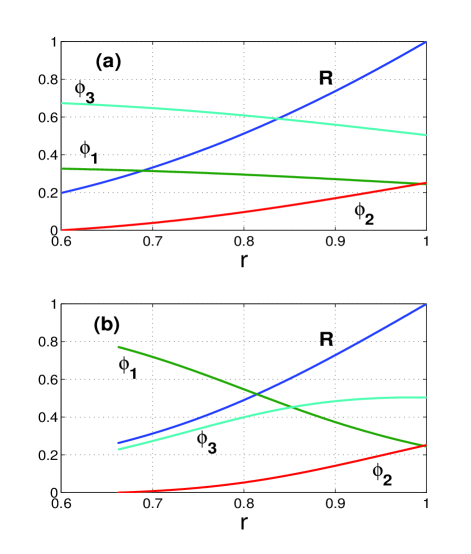
Figure 3: (color online) The curves show the concentrations of the three fluids and the radius $R$ as functions of the physical radial coordinate $r$ for the fluid parameters of Case 1 (see Table 1). (a) the 2D cylindrical configuration; (b) the 3D spherical shell.

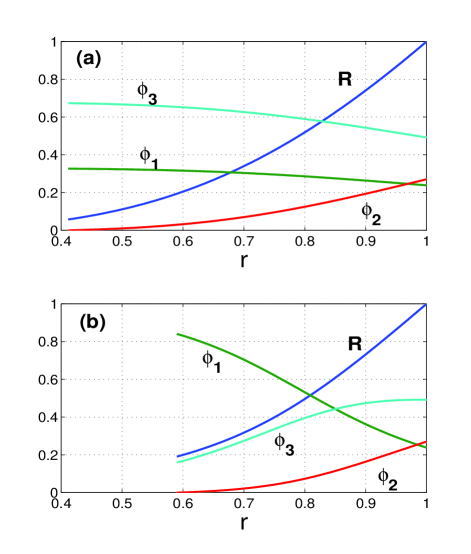
Figure 4: (color online) Case 2. The parameters are the same as in Fig. 3 with the exception that now $S_{3}=0.01$.

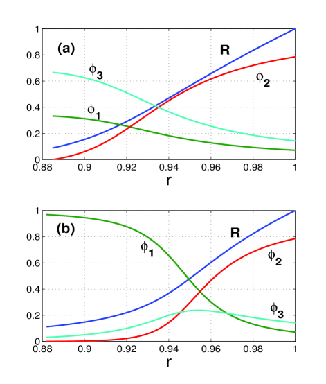
Figure 5: (color online) Case 3. The parameters are the same as in Fig. 4 except that $\rho_{1}=100$, $\rho_{3}=0.02$.

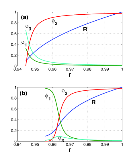
Figure 6: (color online) Case 4. As in Fig. 5 except that now $\rho_{1}=1000$, $\rho_{3}=0.002$.

5.2 Discrete layering algorithm

The inhomogeneous nature of the homogenized material is captured by layering the shell on two scales. The first scale is a fine layering of $L$ distinct bands defined by the regions between $r_{0}<r_{1}<r_{2}<\ldots<r_{L}=r_{out}=1$. The second scale of layering defines three sub-regions between neighboring radii. Let $r_{n,1}\equiv r_{n}$, and define

$$r_{n,m}^{d} =r^{d}_{n,m-1}-\phi_{m-1}(r_{n})\Delta_{n},\quad m=2,3,$$ (35a)

$$\Delta_{n} =r_{n}^{d}-r_{n-1}^{d},\quad n=1,2,\ldots,L,$$ (35b)

where $\frac{\pi}{3}(d+1)\Delta_{n}$ is the area or volume between the inner and outer radii of the band $[r_{n-1},r_{n}]$. The three regions $(r_{n,2},r_{n,1}]$ , $(r_{n,3},r_{n,2}]$ and $(r_{n-1,1},r_{n,3}]$ have fractional volumes $\phi_{1}(r_{n})$, $\phi_{2}(r_{n})$ and $\phi_{3}(r_{n})$ of the band, respectively, and are therefore occupied by the respective fluids, see Fig. 7. The choice of the ordered set $\{r_{n},n=1,2,\ldots,L-1\}$ is relatively arbitrary as long as it is finely spaced for large values of $L$. For simplicity we take $\Delta_{n}$ constant, independent of $n$, in which case $\Delta_{n}=(1-r_{0}^{d})/L\equiv\Delta$ and the radii become

$$r_{n,1}^{d} =r_{0}^{d}+n\Delta,\quad n=1,2,\ldots,L,$$ (36a)

$$r_{n,m}^{d} =r^{d}_{n,m-1}-\phi_{m-1}(r_{n,1})\Delta,\quad m=2,3.$$ (36b)

Table 2: Results for the four cases of Table I. $\bar{\rho}$ is the average density in the shell $r_{0}\leq r\leq 1$. $\sigma_{0}$ is the relative value of the total scattering cross section at $kr_{0}=3$ of a rigid cylinder/sphere surrounded by the 3-fluid shell with 500 layers. A value of $100\%$ corresponds to the bare rigid target.

		2D				3D
	$r_{0}$	$R_{0}$	$\bar{\rho}$	$\sigma_{0}(\%)$	$r_{0}$	$R_{0}$	$\bar{\rho}$	$\sigma_{0}(\%)$
1	0.60	0.20	3.12	25.8	0.66	0.26	5.41	4.55
2	0.41	0.06	3.13	2.37	0.59	0.19	5.69	2.20
3	0.88	0.09	19.17	0.69	0.88	0.11	57.7	.033
4	0.94	0.09	40.22	0.69	0.96	0.096	192	.012

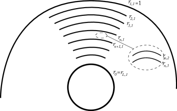
Figure 7: The discrete layering algorithm to reproduce the local homogenization properties of the 3-fluid shell.

5.3 Scattering from a three-fluid shell

We consider plane wave incidence in the uniform exterior fluid $r>1$, with time harmonic dependence $e^{-i\omega t}$ (henceforth omitted). The 3-fluid shell in $r_{0}<r<1$ is defined by the discrete layering algorithm, and is assumed to surround a rigid object of radius $r_{0}$. The scattered pressure is expressed

$$p(r,\theta)=\sum_{n=0}^{\infty}A_{n}\psi_{n}(r)\Lambda_{n}(\theta),$$ (37)

where $\theta$ is the polar angle with respect to the incident direction, $\{\psi_{n}(r),\Lambda_{n}(\theta)\}=\{H_{n}^{(1)}(kr),\cos n\theta\}$ in 2D and $\{h_{n}^{(1)}(kr),P_{n}(\cos\theta)\}$ in 3D, and $k=\omega$ is the nondimensional wavenumber. In the shell region the pressure $p$ and radial velocity $v$ are expressed in modal form

$$\big{(}p(r,\theta),\,v(r,\theta)\big{)}=\sum_{n=0}^{\infty}\big{(}p_{n}(r),\,v_{n}(r)\big{)}\Lambda_{n}(\theta),\quad r_{0}<r<1.$$ (38)

The 2-vector ${\boldsymbol{U}}(r)=\big{(}p_{n}(r),\,r^{d-1}v_{n}(r)\big{)}^{T}$ satisfies the ordinary differential equation (ODE)

$$\frac{\operatorname{d}{\boldsymbol{U}}}{\operatorname{d}r}={\boldsymbol{Q}}(r){\boldsymbol{U}}(r),\quad r_{0}<r<1,$$ (39)

where

$${\boldsymbol{Q}}(r)=\frac{i\omega}{r^{d-1}}\begin{pmatrix}0&\rho\\ r^{2d-4}\big{(}\frac{r^{2}}{K}-\frac{\chi^{2}}{\omega^{2}\rho}\big{)}&0\end{pmatrix},$$ (40)

and $\chi^{2}=n^{2},\,n(n+1)$ in 2D and 3D, respectively. The density $\rho(r)$ and bulk modulus $K(r)$ are piecewise constant, defined by the 3-fluid material properties at each value of $r$ according to the discrete layering algorithm.

5.3.1 Computational scheme

Three different numerical methods are employed to find the scattered pressure (37): (i) by solving for the matricant; (ii) using a global matrix; and (iii) by solving the matricant of the homogenized radially dependent anisotropic fluid. In the first method the matricant Pease (1965), or propagator matrix, is found by numerical integration of the matrix equation $\operatorname{d}{\boldsymbol{M}}/\operatorname{d}r={\boldsymbol{Q}}{\boldsymbol{M}}$ subject to the initial condition ${\boldsymbol{M}}(r_{0})={\boldsymbol{I}}$, the 2$\times$2 identity matrix. Then using the continuity conditions at $r=1$, and the rigid boundary conditions at $r=r_{0}$, it is possible to express the scattering coefficient $A_{n}$ in terms of ${\boldsymbol{M}}(1)$. Solution (ii) using the global matrix method, e.g. Ricks and Schmidt (1994), is obtained by creating a large system of simultaneous equations which can be cast as a matrix equation of size $6L$. The third method (ii) is based on the equations of motion of an anisotropic acoustic fluid, e.g. Norris (2008), with radially varying parameters $\rho_{r}$, $\rho_{\perp}$ and $C_{*}$ given by the exact transformation formulas (3). The equations of motion can be transformed into the form (39) with ${\boldsymbol{Q}}\rightarrow{\boldsymbol{Q}}_{*}$ where

$${\boldsymbol{Q}}_{*}(r)=\frac{i\omega}{r^{d-1}}\begin{pmatrix}0&\rho_{r}\\ r^{2d-4}\big{(}\frac{r^{2}}{K_{*}}-\frac{\chi^{2}}{\omega^{2}\rho_{\perp}}\big{)}&0\end{pmatrix},$$ (41)

and $K_{*}=C_{*}^{-1}$. Using an ODE solver it is again possible to find the scattering coefficient $A_{n}$. Details of numerical schemes (i) and (iii) will be provided in a forthcoming paper.

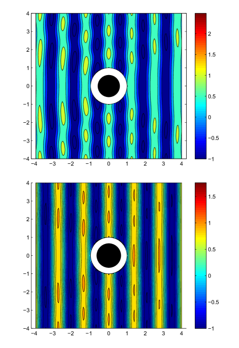
Figure 8: (color online) Case 1. The magnitude of the scattered pressure for an incident wave of unit amplitude for the 2D (top) and 3D (bottom) 3-fluid shells. In each case $kr_{0}=3$ and $L=500$. The inner dark circular region depicts the rigid target of radius $r_{0}$, surrounded by the shell of unit outer radius.

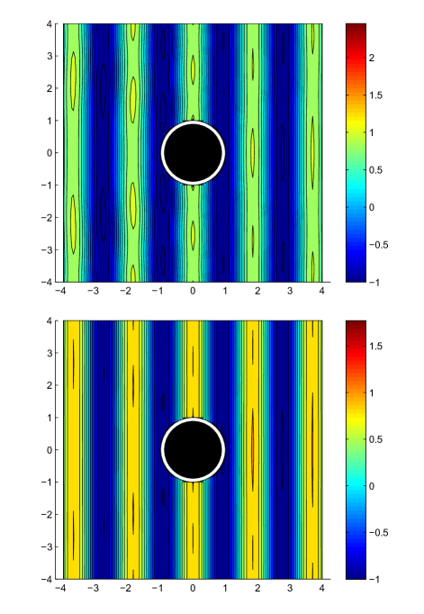
Figure 9: (color online) Case 3. The same as for Figure 8: 2D and 3D simulations are in the upper and lower plots, respectively.

5.3.2 Numerical results

Figures 8 and 9 show the magnitude of the scattered acoustic field for an incident wave of unit amplitude. Since the radius of the object being cloaked changes for each of the four cases of Table I we take the nondimensional characteristic value $kr_{0}=3$ in each scattering simulation. This allows us to compare the total scattering cross-section between the four cases even though the values of $r_{0}$ are different. Fig. 10 shows the response of the bare 3D spherical rigid target based upon case 3 in which $r_{0}=.88$. The total scattering cross-section for the “cloaked” rigid object was calculated using the coefficients $A_{n}$, and compared with the cross-section for the bare rigid object. In each case, as Table II shows, the relative cross-section is diminished, and for cases 3 and 4 the reduction is significant. Note that the reduction in target strength is greater in 3D as compared with 2D, in agreement with the general findings of Norris (2008). The numerical methods (i) and (ii) were found to be in agreement with one another, and with method (iii) when $L$ is very large. For instance, the cross-section found using method (iii) is $0.3\%$ larger than that of method (i) for the 2D example in Fig. 8. Finally Fig. 11 shows the effect of the number of layers $L$ on the relative value of the total scattering cross section for case 3. A curve fit of the power function $aL^{b}+c$ shows that for this particular case at this particular frequency the cross-section decreases as $\sigma_{0}\sim L^{-2.2}$. More layers provide a better approximation to the homogenized limit, as expected. For small numbers of layers the layering algorithm used here could be improved using various optimization strategies, but we do not pursue that here.

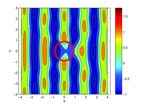
Figure 10: (color online) 3D pressure map solution for a rigid cylinder; $kr_{0}=3$, $r_{0}=.88$.

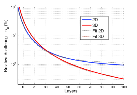
Figure 11: (color online) The relative value of the total scattering cross section for case 3 vs. the number of three-fluid layers in $r_{0}<r\leq 1$. The dashed lines are curve fits of the form $aL^{b}+c$ for $5\leq L\leq 100$. The parameters $(a,b,c)$ and the root mean squared error (RMSE) were found to be $(3716,-2.221,0.9924)$, $0.290$ for 2D, and $(6435,-2.258,0.1324)$, $0.278$ for 3D.

6 Conclusion

The main finding of this paper is that it is possible to achieve cloaking-like behavior with as few as three distinct acoustic fluids. Using transformation acoustics, we find that for a given set of three fluids the layered shell $r_{0}<r<1$ is uniquely determined, with the inner radius $r_{0}$ given by eqs. (17) and (19) for 2D and 3D, respectively. The shell is made of fine layers of the three fluids with relative concentrations as a function of $r$ determined from eqs. (3), (6a) and (9). Obviously, the overall effectiveness and the precise form of the layering depends upon the relative densities and compressibilities of the three fluids. The best results are obtained if one fluid has density equal or close to the background or host fluid density, while the other two densities are much greater and much less than the background value. Numerical simulations of the scattering from specific layering realizations confirm the theoretical predictions and show the effect of the finite number of layers. Many questions remain as to the the optimal choice of fluids in general, and what can be achieved using existing fluids specifically.

Appendix A Properties of the 2D 3-fluid material

A.1 Density and compressibility

We begin with the density implications. Equation (6a) reduces, using $\rho_{r}\rho_{\perp}=1$, to give

$$\phi_{i}=\frac{\rho_{i}(\rho_{j}+\rho_{k})(\rho_{r}-\rho_{ri})}{\rho_{ri}(\rho_{i}-\rho_{j})(\rho_{i}-\rho_{k})},\quad i\neq j\neq k\neq i,$$ (42)

where the critical values of $\rho_{r}$ are given by (18). Based upon the identities (42), we note that

$$\left.\phi_{i}\right|_{\rho_{r}=\rho_{ri}}=0,\quad\left.\phi_{j}\right|_{\rho_{r}=\rho_{ri}}=\rho_{j}\rho_{ri}\bigg{(}\frac{1-\rho_{k}^{2}}{\rho_{j}^{2}-\rho_{k}^{2}}\bigg{)},$$ (43)

where $i\neq j\neq k\neq i$. The points defined by (43) are the intersections of the line (42) with the planes ${\boldsymbol{e}}_{i}\cdot{\boldsymbol{\phi}}=0$. In order to have some ${\boldsymbol{\phi}}\in\Phi_{3}$ at least one of the intersections must lie on the boundary of $\Phi_{3}$. Consider $\rho_{ri}$ of (18), then $\phi_{j}$ and $\phi_{k}$ must both be positive, which occurs if and only if one of $(\rho_{j},\rho_{k})$ is larger than, and the other is less than, unity. This gives an important necessary condition: At least one of the three densities is larger than unity, and conversely, at least one must be less than unity. This condition must hold in addition to the obvious requirement that the three densities are distinct, since otherwise the system (5) is not solvable.

Introduce the density values $\rho_{p}$, $\rho_{m}$, $\{p\neq m\}\in\{1,3\}$, such that

$$(\rho_{2}-1)(\rho_{p}-1)>0,\quad(\rho_{2}-1)(\rho_{m}-1)<0,$$ (44)

with $2\neq p\neq m\neq 2$.

We note some other properties of the critical values of the densities:

$$\rho_{ri}-\rho_{rj} =\rho_{ri}\rho_{rj}\frac{(\rho_{j}-\rho_{i})(1-\rho_{k}^{2})}{(\rho_{i}+\rho_{k})(\rho_{j}+\rho_{k})},$$ (45a)

$$\rho_{ri}-1 =-\rho_{ri}\frac{(\rho_{rj}-1)(1-\rho_{rk})}{\rho_{rj}+\rho_{rk}},$$ (45b)

where $i\neq j\neq k\neq i$. These imply, respectively, that $\rho_{r2}>\rho_{rp}>\rho_{rm}$, and $\rho_{r2}>1$, $\rho_{rp}>1$ and $\rho_{rm}<1$. Combining these with the previous inequalities, we surmise the ordering $\rho_{r2}>\rho_{rp}>1>\rho_{rm}$. Thus, for instance, if $\rho_{2}>1$, then the possible range of $\rho_{r}$ is $\rho_{r1}\leq\rho_{r}\leq\rho_{r2}$. If $\rho_{2}<1$ then it is $\rho_{r3}\leq\rho_{r}\leq\rho_{r2}$.

Any value of $\rho_{r}$ in the range $\rho_{rp}\leq\rho_{r}\leq\rho_{r2}$ therefore yields a triple of concentration values satisfying ${\boldsymbol{\phi}}\in\Phi_{3}$. At the upper (lower) value, $\rho_{r}=\rho_{r2}$ $(=\rho_{rp})$, the concentration ${\boldsymbol{\phi}}$ lies on the boundary of the triangle with $\phi_{2}=0$ $(\phi_{p}=0)$. But these limiting values are not necessarily achieved. Thus, at $r=R=1$ the differential equality (9) implies that $\rho_{r}=\alpha/(1-\beta)$, see eq. (50). This is the practical lower bound on the range of $\rho_{r}$. Equations (24) and (25)₁ then follow.

By analogy with equation (24) for the volume fractions, the effective compressibility of (6b) can be expressed in the form (24b). Alternatively, eq. (6b) implies $C_{*}=\alpha+\beta\rho_{r}$, and therefore we deduce that $\alpha$ and $\beta$ may be expressed

$$\alpha=\frac{\rho_{r2}C_{*\,p}-\rho_{rp}C_{*\,2}}{\rho_{r2}-\rho_{rp}},\quad\beta=\frac{C_{*\,2}-C_{*\,p}}{\rho_{r2}-\rho_{rp}}.$$ (46)

These lead in turn to explicit expressions for the two parameters that define the transformation function, (12),

$$\lambda =S_{1}\frac{(1-\rho_{2})(1-\rho_{3})}{(\rho_{1}-\rho_{2})(\rho_{1}-\rho_{3})}+S_{2}\frac{(1-\rho_{3})(1-\rho_{1})}{(\rho_{2}-\rho_{3})(\rho_{2}-\rho_{1})}$$

$$\quad+S_{3}\frac{(1-\rho_{1})(1-\rho_{2})}{(\rho_{3}-\rho_{1})(\rho_{3}-\rho_{2})},$$ (47)

$$\mu =\frac{\rho_{r1}^{-1}S_{1}(\rho_{2}^{2}-\rho_{3}^{2})+\rho_{r2}^{-1}S_{2}(\rho_{3}^{2}-\rho_{1}^{2})+\rho_{r3}^{-1}S_{3}(\rho_{1}^{2}-\rho_{2}^{2})}{S_{1}(\rho_{2}^{2}-\rho_{3}^{2})+S_{2}(\rho_{3}^{2}-\rho_{1}^{2})+S_{3}(\rho_{1}^{2}-\rho_{2}^{2})},$$

where $S_{i}=\rho_{i}C_{i}$, $i=1,2,3$.

A.1.1 Sensitivity

The reachable range of $\rho_{r}$ is, from (9), $\rho_{rp}<\rho_{r}<\rho_{rp}+\Delta\rho_{r}$ where

$$\Delta\rho_{r}\equiv\rho_{r2}-\rho_{rp}=\frac{(\rho_{p}-\rho_{2})(1-\rho_{m}^{2})}{(1+\rho_{2}\rho_{m})(1+\rho_{p}\rho_{m})}.$$ (48)

Hence,

$$\frac{\partial\Delta\rho_{r}}{\partial\rho_{2}} =-\frac{(1-\rho_{m}^{2})}{(1+\rho_{2}\rho_{m})^{2}},$$

$$\frac{\partial\Delta\rho_{r}}{\partial\rho_{p}} =\frac{(1-\rho_{m}^{2})}{(1+\rho_{p}\rho_{m})^{2}},$$ (49)

$$\frac{\partial\Delta\rho_{r}}{\partial\rho_{m}} =-\frac{(\rho_{p}-\rho_{2})(1+\rho_{m}^{2})(\rho_{2}+\rho_{p}+2\rho_{2}\rho_{p}\rho_{m})}{(1+\rho_{2}\rho_{m})^{2}(1+\rho_{p}\rho_{m})^{2}}.$$

If $p=1$ these are, respectively, $<0$, $>0$, $<0$. Conversely, if $p=1$ they are $>0$, $<0$, $>0$. Hence, whether $p=1$ or $p=3$ it is clear that $\Delta\rho_{r}$ is greatest if $\rho_{1}$ is large, $\rho_{2}$ is close to unity, and $\rho_{3}$ is small.

A.2 Transformation function

A.2.1 Necessary conditions for the three-fluid parameters

Since $R(1)=1$ at the outer radius $r=1$, we have

$$R^{\prime}(1)=\rho_{r}(1)=C_{*}(1)=\frac{\alpha}{1-\beta},$$ (50)

that is,

$$\rho_{r}(1)=C_{*}(1)=\frac{\rho_{r2}C_{*p}-\rho_{rp}C_{*2}}{\rho_{r2}-\rho_{rp}+C_{*p}-C_{*2}}.$$ (51)

But we require that $\rho_{rp}\leq\rho_{r}(1)\leq\rho_{r2}$, or, since $\rho_{r2}-\rho_{rp}>0$,

$$\begin{split}\frac{\rho_{r}(1)-\rho_{rp}}{\rho_{r2}-\rho_{rp}}&=\frac{C_{*p}-\rho_{rp}}{\rho_{r2}-\rho_{rp}+C_{*p}-C_{*2}}>0,\\ \frac{\rho_{r2}-\rho_{r}(1)}{\rho_{r2}-\rho_{rp}}&=\frac{\rho_{r2}-C_{*2}}{\rho_{r2}-\rho_{rp}+C_{*p}-C_{*2}}>0.\end{split}$$ (52)

Hence, (28) must hold, or, explicitly

$$\big{(}S_{1}\frac{1-\rho_{3}^{2}}{\rho_{1}^{2}-\rho_{3}^{2}}+S_{3}\frac{\rho_{1}^{2}-1}{\rho_{1}^{2}-\rho_{3}^{2}}-1\big{)}\times$$

$$\big{(}S_{2}\frac{1-\rho_{m}^{2}}{\rho_{2}^{2}-\rho_{m}^{2}}+S_{m}\frac{\rho_{2}^{2}-1}{\rho_{2}^{2}-\rho_{m}^{2}}-1\big{)}<0.$$ (53)

A.2.2 The case $\rho_{2}=1$

In this case the $p/m$ distinction is unnecessary since

$$\rho_{r1}=\rho_{r3}=1\text{ for }\rho_{2}=1,\,\Rightarrow\,{\boldsymbol{\phi}}\in\Phi_{3}\,\text{ for }1\leq\rho_{r}\leq\rho_{r2}.$$

This implies that the reachable quantities reduce to (29a).

Appendix B The two fluid material

B.1 General theory

The 2-fluid version of eq. (5) is

$$\begin{pmatrix}1&1\\ \rho_{1}&\rho_{2}\\ \frac{1}{\rho_{1}}&\frac{1}{\rho_{2}}\end{pmatrix}\begin{pmatrix}\phi_{1}\\ \phi_{2}\end{pmatrix}=\begin{pmatrix}1\\ \rho_{r}\\ \rho_{\perp}^{-1}\end{pmatrix}.$$ (54)

This implies that the concentrations are

$$\phi_{1}=\frac{\rho_{r}-\rho_{2}}{\rho_{1}-\rho_{2}},\qquad\phi_{2}=\frac{\rho_{1}-\rho_{r}}{\rho_{1}-\rho_{2}},$$ (55)

and the densities $\rho_{r}$, $\rho_{\perp}$ are related by the compatibility condition for (54),

$$\rho_{r}+\rho_{1}\rho_{2}\rho_{\perp}^{-1}=\rho_{1}+\rho_{2}.$$ (56)

The effective compressibility, which follows from (55) and the third relation in (1), satisfies

$$(\rho_{1}-\rho_{2})C_{*}+(C_{2}-C_{1})\rho_{r}=\rho_{1}C_{2}-\rho_{2}C_{1}.$$ (57)

Equation (55) provides relations for the volume fractions in terms of the radial inertia $\rho_{r}$. One can also interpret eqs. (56) and (57) as defining $\rho_{\perp}$ and $C_{*}$, respectively, in terms of $\rho_{r}$. Therefore, all parameters in the two-fluid material can be defined by a single quantity, in this case $\rho_{r}$.

However, in order to relate the two-fluid material to a transformation it is necessary that there exists a function $R$ which satisfies the three differential identities (3). Substitution of these into eqs. (56) and (57) gives a pair of equations which can be considered as algebraic equations in two unknowns: $R^{\prime}$ and $R/r$. Solutions for both of these quantities can be found in terms of the two-fluid properties $\rho_{1},\rho_{2},C_{1},C_{2}$, but the solutions are not of practical interest. The reason is that the constant values of $R^{\prime}$ and $R/r$ that are found, say $R^{\prime}=a$, $R/r=b$, must be equal, leading to trivial cases. The main conclusion from the study of the $N=2$ case is that the 2-fluid material is overly restrictive.

B.2 A special case of a uniform 2-fluid material

While it is not possible for the 2-fluid material to reproduce a transformation material, it is possible to make some interesting uniform fluids with anisotropic inertia. The idea is to seek constant values of $\rho_{r}$, $\rho_{\perp}$ and $C_{*}$ which also match to the exterior fluid in $r>1$. This requires that $R=1$ at $r=1$. Enforcement of (3) then requires the three parameters in the left vector be equal to $R^{\prime}$. Substituting into eqs. (56) yields

$$\rho_{r}=\rho_{\perp}^{-1}=C_{*}=\rho_{r3}.$$ (58)

The volume fractions follow from (55) as

$$\phi_{1}=\rho_{1}\rho_{r3}\bigg{(}\frac{1-\rho_{2}^{2}}{\rho_{1}^{2}-\rho_{2}^{2}}\bigg{)},\quad\phi_{2}=\rho_{2}\rho_{r3}\bigg{(}\frac{1-\rho_{1}^{2}}{\rho_{2}^{2}-\rho_{1}^{2}}\bigg{)},$$ (59)

which are both positive if and only if $(1-\rho_{1})(1-\rho_{2})<0$. The one remaining condition, for the compressibility, implies using (57) and (58) that the two compressibilities must be related such that

$$C_{1}\rho_{1}(1-\rho_{2}^{2})+C_{2}\rho_{2}(\rho_{1}^{2}-1)=\rho_{1}^{2}-\rho_{2}^{2}.$$ (60)

The anisotropic fluid (58) is defined by the parameter $\rho_{r3}=\rho_{r3}(\rho_{1},\rho_{2})$, and is composed of volume fractions $\phi_{i}=\phi_{i}(\rho_{1},\rho_{2})$ of fluid $i=1,2$. Denote any pair satisfying the relation (60) as $C_{i}=C_{i}(\rho_{1},\rho_{2})$, $i=1,2$. It is interesting to note that these functions are invariant under the interchange $\{\rho_{1},\rho_{2},\phi_{1},\phi_{2},C_{1},C_{2}\}\rightarrow\{\rho_{2}^{-1},\rho_{1}^{-1},\phi_{2},\phi_{1},C_{2},C_{1}\}$.

B.2.1 Examples

If, for instance, $C_{1}\rho_{1}=C_{2}\rho_{2}$ then (60) implies that $C_{1}\rho_{1}=C_{2}\rho_{2}=1$. Both fluids have the same wave speed as the background fluid. They differ only in their impedances, which in this case are $z_{i}=\rho_{i}=C_{i}^{-1}$, $i=1,2$.

Conversely, if $C_{1}/\rho_{1}=C_{2}/\rho_{2}$ then (60) implies that $C_{1}/\rho_{1}=C_{2}/\rho_{2}=1$. The two fluids have the same acoustic impedance as the background fluid, and differ only in their wave speeds, which are $c_{i}=\rho_{i}^{-1}=C_{i}^{-1}$, $i=1,2$.

B.3 A two and a half fluid material

As a case intermediate between the strictly 2-fluid and 3-fluid cases, consider the 2D case, for which $(r/R)R^{\prime}=\rho_{r}$, see (3)₁. It follows from (56)₂, i.e. $\rho_{r}=\rho_{\perp}^{-1}$, that $\rho_{r}=\rho_{r3}$, a constant. Taking into account the boundary condition $R(1)=1$, the unique mapping is

$$R(r)=r^{\rho_{r3}}.$$ (61)

Equation (57) combined with (3)₃ then implies

$$(1-\rho_{2}^{2})S_{1}+(\rho_{1}^{2}-1)S_{2}=(\rho_{1}^{2}-\rho_{2}^{2})r^{2(\rho_{r3}-1)}.$$ (62)

This cannot be satisfied if the two fluids have properties independent of $r$. However, if we still require that the densities are fixed, but the compressibilities could vary with $r$, then (62) suggests that a mapping can be realized if one or both $S_{1}$, $S_{2}$ are such that the equality holds for some range of $r$. It is well known that adding a small concentration of bubbles to a liquid results in an increase in the compressibility without significant change in the effective density. Hence, it might be possible, in principle if not in practice, to add a third fluid whose only role is to enhance compressibility. In this sense it is half of a fluid, since its inertial properties are not used.

References

- Norris (2009) A. N. Norris. Acoustic metafluids. J. Acoust. Soc. Am., 125(2):839–849, 2009. 10.1121/1.2817359.
- Pendry et al. (2006) J. B. Pendry, D. Schurig, and D. R. Smith. Controlling electromagnetic fields. Science, 312(5781):1780–1782, June 2006. 10.1126/science.1125907.
- Cummer and Schurig (2007) S. A. Cummer and D. Schurig. One path to acoustic cloaking. New J. Phys., 9(3):45+, March 2007. 10.1088/1367-2630/9/3/045.
- Chen and Chan (2007) H. Chen and C. T. Chan. Acoustic cloaking in three dimensions using acoustic metamaterials. Appl. Phys. Lett., 91(18):183518+, 2007. 10.1063/1.2803315.
- Norris (2008) A. N. Norris. Acoustic cloaking theory. Proc. R. Soc. A, 464:2411–2434, 2008. 10.1098/rspa.2008.0076.
- Torrent and Sánchez-Dehesa (2008) D. Torrent and J. Sánchez-Dehesa. Acoustic cloaking in two dimensions: a feasible approach. New J. Phys., 10(6):063015+, June 2008. 10.1088/1367-2630/10/6/063015.
- Schoenberg and Sen (1983) M. Schoenberg and P. N. Sen. Properties of a periodically stratified acoustic half-space and its relation to a Biot fluid. J. Acoust. Soc. Am., 73(1):61–67, 1983. 10.1121/1.388724.
- Pease (1965) M. C. Pease. Methods of Matrix Algebra, 172–176. Academic Press, New York, 1965.
- Ricks and Schmidt (1994) D. C. Ricks and H. Schmidt. A numerically stable global matrix method for cylindrically layered shells excited by ring forces. J. Acoust. Soc. Am., 95(6):3339–3349, 1994.