Noncoplanar magnetic ordering driven by itinerant electrons on the pyrochlore lattice

Abstract

Exchange interaction tends to favor collinear or coplanar magnetic orders in rotationally invariant spin systems. Indeed, such magnetic structures are usually selected by thermal or quantum fluctuations in highly frustrated magnets. Here we show that a complex noncoplanar magnetic order with a quadrupled unit cell is stabilized by itinerant electrons on the pyrochlore lattice. Specifically we consider the Kondo-lattice and Hubbard models at quarter filling. The electron Fermi ‘surface’ at this filling factor is topologically equivalent to three intersecting Fermi circles. Perfect nesting of the Fermi lines leads to magnetic ordering with multiple wavevectors and a definite handedness. The chiral order might persist without magnetic order in a chiral spin liquid at finite temperatures.

Magnets with geometrical frustration have fascinated physicists for more than a decade as models of strongly interacting systems. A prominent example of magnetic frustration in high dimensions is the nearest-neighbor antiferromagnet on the pyrochlore lattice shown in Fig. 1(a). For classical Heisenberg spins, strong geometrical frustration prevents the magnet from settling in a long-range magnetic order even at zero temperature moessner98 . Instead, the ground state retains a finite zero-point entropy and is susceptible to small perturbations such as anisotropies, further-neighbor couplings, and dipolar interactions. In real compounds, magnetic frustration is often relieved when spins couple to other degrees of freedom. An intensively studied case is spin-lattice coupling in chromium spinels where the magnetic transition is accompanied by a lattice distortion lee00 ; ot02 ; chern06 . Another well known example is magnetic phase transition faciliated by orbital order in frustrated spin-orbital systems lee04 ; garlea08 ; ot04 ; chern09 .

Metallic pyrochlore magnets such as Kondo-lattice or double-exchange models pose a different challenge for theorists due to the nonlocal nature of the electron-mediated interactions. Indeed, despite considerable effort ikoma03 ; ikeda08 ; motome10 ; lacroix , a complete picture of the phase diagram is still lacking. An early study of the double-exchange model on pyrochlore lattice revealed a rich mean-field phase diagram ikoma03 . However, the calculation only considered magnetic orders which preserve the lattice translational symmetry, hence precluding magnetic structures with multiple wavevectors. A recent Monte Carlo study of the same model provided an unbiased phase diagram at large Hund’s coupling motome10 . In particular, a peculiar state with electronic phase separation was observed. Magnetic orders in the weak-coupling regime remain unclear.

Magnetic ordering in frustrated metallic systems depends in an intricate way on the underlying electron Fermi surface. At small filling factors, localized spins interact with each other through a long-range oscillatory Ruderman-Kittel-Kasuya-Yosida (RKKY) interaction mediated by the electrons. A Monte Carlo simulation of pyrochlore spin-ice with RKKY interaction showed that the sign of the effective Curie-Weiss constant as well as that of nearest-neighbor coupling vary with the electron Fermi wavevector ikeda08 . This in turn determines magnetic ordering at low temperatures: the magnetic state of individual tetrahedra evolves from the all-in all-out structure to the 2-in 2-out ferromagnetic state with increasing electron density.

The geometry of the electron Fermi surface also plays an important role in determining the magnetic instability of itinerant systems, particularly at commensurate filling factors. A canonical example is Néel ordering caused by perfect Fermi surface nesting that occurs at a half-filled square-lattice Hubbard model. While the resulting spin structure is collinear in bipartite square lattice, it was shown that nesting effect on triangular lattice leads to a rare noncoplanar magnetic order at filling factors $3/4$ and $1/4$ martin08 ; akagi10 ; kato10 . This chiral magnetic structure induces a spontaneous quantum Hall effect in the absence of external magnetic field. Although a long-range magnetic order cannot survive thermal fluctuations in two spatial dimensions, the discrete chirality order persists up to a finite temperature martin08 .

In this paper we demonstrate that the ground state of an isotropic Kondo-lattice model on the pyrochlore lattice is magnetically ordered with a noncoplanar spin structure and a definite chirality. The conclusion also applies to Hubbard model on the pyrochlore lattice at the mean-field level. The noncoplanar magnetic order stems from a weak-coupling instability caused by perfect nesting of Fermi ‘circles’ at quarter filling; the quadrupled magnetic unit cell contains 16 spins. In contrast to the triangular-lattice model martin08 , this noncoplanar spin order does not support a spontaneous Hall insulator because of a trivial Berry phase acquired by the electrons when traversing a tetrahedron. The magnetic structure itself, on the other and, has a definite handedness and is characterized by a nonzero chiral order parameter.

It should be pointed out that although chiral magnetic orders have been reported in metallic pyrochlore oxides such as Pr₂Ir₂O₇ nakatsuji , the non-coplanarity of spins in these so called spin-ice compounds are mainly created by a strong uniaxial anisotropy. The electron-driven magnetic instability in pyrochlore spin-ice at quarter filling will be briefly discussed at the end of the paper.

We begin with the isotropic Kondo-lattice Hamiltonian on the pyrochlore lattice:

$$H = -t\sum_{\langle ij\rangle}\left(c^{\dagger}_{i\alpha}\,c^{\phantom{\dagger}}_{j\alpha}+\mbox{h.c.}\right)+J\sum_{\langle ij\rangle}\mathbf{S}_{i}\cdot\mathbf{S}_{j}$$ (1)

$$\!+\,\,K\sum_{i}\mathbf{S}_{i}\cdot c^{\dagger}_{i\alpha}\bm{\sigma}^{\phantom{\dagger}}_{\alpha\beta}c^{\phantom{\dagger}}_{i\beta}.$$

The first term describes electron hopping between nearest-neighbor sites, $t$ is the hopping integral, and $c^{\dagger}_{i\alpha}$ creates an electron with spin $\alpha$ on site $i$. The second term represents the superexchange interaction between neighboring localized spins $\mathbf{S}_{i}$. The itinerant electrons interact with the localized spins through an on-site exchange coupling $K$; the vector $\bm{\sigma}_{\alpha\beta}$ denotes the three Pauli matrices. We consider the classical limit of localized spins with magnitude $|\mathbf{S}_{i}|=S\gg 1$. In this classical limit, the electron spectrum is independent of the sign of $K$ and the eigenstates of opposite signs are connected by a global gauge transformation martin08 .

We first consider the tight-binding spectrum of electrons on the pyrochlore lattice. In momentum space, the hopping Hamiltonian [first term in Eq. (1)] is expressed as $H_{t}=\sum_{m,n}\sum_{\mathbf{k},\alpha}\tau_{mn}(\mathbf{k})\,c^{\dagger}_{m\alpha}(\mathbf{k})\,c_{n\alpha}(\mathbf{k}),$ where $m,n$ are sublattice indices and the hopping matrix is

$$\tau(\mathbf{k})=-2\,t\left(\begin{array}[]{cccc}\mbox{\small 0}&c_{yz}&c_{zx}&c_{xy}\\ c_{yz}&\mbox{\small 0}&\bar{c}_{xy}&\bar{c}_{zx}\\ c_{zx}&\bar{c}_{xy}&\mbox{\small 0}&\bar{c}_{yz}\\ c_{xy}&\bar{c}_{zx}&\bar{c}_{yz}&\mbox{\small 0}\end{array}\right).$$ (6)

Here we have introduced $c_{ab}=\cos\left[(k_{a}+k_{b})/4\right]$ and $\bar{c}_{ab}=\cos\left[(k_{a}-k_{b})/4\right]$ and set the length of a cubic unit cell $a=1$. This hopping matrix can be exactly diagonalized, giving rise to a spectrum shown in Fig. 1(d). It consists of two degenerate flat bands $\varepsilon^{\rm flat}_{\mathbf{k}}=2t$ and two dispersive bands:

$$\varepsilon^{\pm}_{\mathbf{k}}=-2\,t\left(1\mp\sqrt{1+\mathcal{Q}_{\mathbf{k}}}\right),$$ (7)

where $\mathcal{Q}_{\mathbf{k}}=\cos\frac{k_{x}}{2}\cos\frac{k_{y}}{2}+\cos\frac{k_{y}}{2}\cos\frac{k_{z}}{2}+\cos\frac{k_{z}}{2}\cos\frac{k_{x}}{2}.$ These two branches touch each other along the diagonal lines of the square faces of the Brillouin zone [Fig. 1(b)].

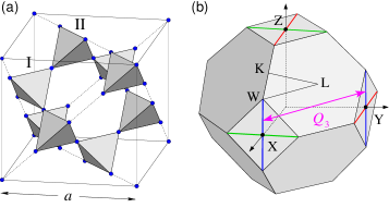
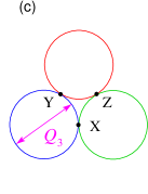
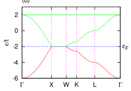
Figure 1: (a) A conventional cubic unit cell of the pyrochlore lattice. I and II denote the two types of tetrahedra with different orientations. (b) First Brillouin zone of the fcc lattice. At quarter filling, the electron Fermi ‘surface’ consists of diagonal lines on the square face of the Brillouin zone. (c) Topologically, these Fermi lines are equivalent to three closed loops interceting at the X points of the Brillouin zone. (d) Band structure of the tight-binding model on pyrochlore lattice. The segment XW corresponds to one-quarter of a Fermi line at quarter filling.

At quarter filling the lowest band $\varepsilon^{-}_{\mathbf{k}}$ is completely filled. The corresponding Fermi ‘surface’ is determined by $\varepsilon^{+}_{\mathbf{k}}=\varepsilon^{-}_{\mathbf{k}}$ and consists of diagonal lines $2\pi(x,0,1)$, and so on, on the square faces of the zone boundary. The Fermi energy lies exactly at $E_{F}=-2t$. Noting that $2\pi(x,0,1)\equiv 2\pi(1-x,1,0)$ module a reciprocal lattice vector, these diagonal lines are topologically equivalent to three closed loops, or circles, intersecting with each other at the X points of the Brillouin zone [Fig. 1(b–c)]. In the vicinity of these Fermi lines, the spectrum has the form $\varepsilon^{\pm}_{\mathbf{k}}\approx E_{F}\pm C_{\varphi}\times|\mathbf{k}_{\perp}|$, where $\mathbf{k}_{\perp}$ is the perpendicular component of electron momentum.

The reduction of Fermi surface to Fermi lines at quarter filling also makes it possible to realize perfect nesting with a few wavevectors. Indeed, the three Fermi circles can be perfectly nested by wavevectors $\mathbf{Q}_{1}=2\pi(1,0,0)$, $\mathbf{Q}_{2}=2\pi(0,1,0)$, and $\mathbf{Q}_{3}=2\pi(0,0,1)$, respectively. For example, states on the two Fermi lines $2\pi(1,0,z)$ and $2\pi(0,1,z)$, both belonging to the blue Fermi circle in Fig. 1(c), differ by $\mathbf{Q}_{3}$ up to a reciprocal lattice vector. The Van Hove singularity of the density of states at the Fermi level gives rise to a logarithmically divergent Lindhard susceptibility: $\chi(\mathbf{q})\sim-\log|\mathbf{q}-\mathbf{Q}_{\eta}|$, indicating a weak-coupling instability caused by the nesting effect.

To investigate possible magnetic ordering caused by perfect nesting of the Fermi lines, we consider spin orders which can be expanded as

$$\mathbf{S}_{i}=\mathbf{S}_{m}(\mathbf{r})=\sum_{\eta=0}^{3}\mathbf{M}_{m,\eta}\,e^{i\mathbf{Q}_{\eta}\cdot\mathbf{r}},$$ (8)

where $m$ is the sublattice index and $\mathbf{r}$ denotes the position of the Bravais (fcc) lattice point. In order to accommodate, e.g. ferromagnetic ordering, we have included a $\mathbf{Q}_{0}=0$ component in the above expansion. The unit cell of this multiple-$\mathbf{Q}$ magnetic order is extended to the conventional cubic unit cell which contains 16 inequivalent spins.

Next we include the on-site Hund’s exchange which couples electron with momentum $\mathbf{k}$ to that with $\mathbf{k}+\mathbf{Q}_{\eta}$. After Fourier transformation, the on-site coupling term has the form

$$H_{K}=\sum_{\xi,\eta}\sum_{\alpha,\beta}\sum_{m,\mathbf{k}}\!^{\prime}\,c^{\dagger}_{m\alpha}(\mathbf{k}\!+\!\mathbf{Q}_{\xi})\,\,\mathcal{M}^{(m)}_{\xi\alpha,\eta\beta}\,\,c^{\phantom{\dagger}}_{m\beta}(\mathbf{k}\!+\!\mathbf{Q}_{\eta}).\,\,\,$$ (9)

Here the prime indicates that the momentum summation is restricted to the reduced Brillouin zone, and the coupling coefficients are given by

$$\mathcal{M}^{(m)}_{\xi\alpha,\eta\beta}=K\,\Delta_{\xi\eta,\,\zeta}\,(\mathbf{M}_{m,\zeta}\cdot\bm{\sigma}_{\alpha\beta})\,e^{i(\mathbf{Q}_{\xi}-\mathbf{Q}_{\eta})\cdot\mathbf{d}_{m}},$$ (10)

where $\mathbf{d}_{m}$ denotes basis vectors of the pyrochlore lattice. Momentum conservation of the coupling is encoded in the symbol $\Delta_{\xi\eta,\,\zeta}$ which is symmetric with respect to the first two indices. The nonzero components include $\Delta_{01,1}=\Delta_{02,2}=\Delta_{03,3}=\Delta_{23,1}=\Delta_{31,2}=\Delta_{12,3}=1$.

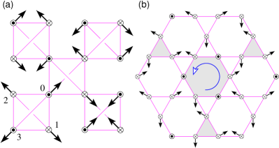
Figure 2: (a) A unit cell of the noncoplanar magnetic order viewed from the $c$ axis. Here we choose $\hat{\mathbf{n}}_{1}=\hat{\mathbf{a}}$, $\hat{\mathbf{n}}_{2}=\hat{\mathbf{b}}$, and $\hat{\mathbf{n}}_{3}=\hat{\mathbf{c}}$ in Eq. (11). (b) Chiral structure of the same magnetic order projected onto a $(111)$ kagome plane. The $\odot$ and $\otimes$ symbols denote spin component coming out of and into the plane, respectively. Same handedness (right-handed in this case) is observed in other kagome planes.

For a given set of Fourier components $\mathbf{M}_{m,\eta}$, diagonalization of the electron Hamiltonian $H_{t}+H_{K}$ gives a total of 32 energy bands. Due to perfect nesting of Fermi lines, the first 8 bands are expected to be separated from other high energy states by an energy gap. At quarter filling, the ground-state energy of electrons $E_{e}$ is obtained by filling the lowest eight bands. However, the determination of the minimum-energy state is not straightforward because of the large number of variables required to describe the spin structure. Indeed, even restricting to magnetic orders which can be expressed in the form of Eq. (8), one still needs 32 variables to specify the 16 classical spins in a quadrupled unit cell. Here we employ the simulated annealing algorithm to minimize the energy functional $E_{e}\left(\mathbf{M}_{m,\eta}\right)$. For Hund’s coupling below a critical value $K_{c}\approx 4.32\,t$ and $J=0$, we obtained the same noncoplanar magnetic order shown in Fig. 2 using different initial configurations and rates of decreasing the effective temperature. For $K>K_{c}$ ferromagnetic order with $\mathbf{S}_{i}=S\,\hat{\mathbf{n}}$ takes over and becomes the ground state.

To characterize the noncoplanar spin structure, we introduce three order parameters $\mathbf{L}_{1}=(\mathbf{S}_{0}+\mathbf{S}_{1}-\mathbf{S}_{2}-\mathbf{S}_{3})/4S$, and so on chern06 , which measure the staggered magnetizations of a tetrahedron; the spin subscript indicates the corresponding sublattice. A unit cell of the magnetic order is shown in Fig. 2(a), where the magnetic states of type-I tetrahedra are described by order parameters

$$\mathbf{L}_{1}=\frac{\hat{\mathbf{n}}_{1}}{\sqrt{3}}\,e^{i\mathbf{Q}_{3}\cdot\mathbf{r}},\,\,\,\,\mathbf{L}_{2}=\frac{\hat{\mathbf{n}}_{2}}{\sqrt{3}}\,e^{i\mathbf{Q}_{1}\cdot\mathbf{r}},\,\,\,\,\mathbf{L}_{3}=\frac{\hat{\mathbf{n}}_{3}}{\sqrt{3}}\,e^{i\mathbf{Q}_{2}\cdot\mathbf{r}}.\,\,$$ (11)

Here $\hat{\mathbf{n}}_{r}$’s are three mutually orthogonal unit vectors. Remarkably, the noncoplanar magnetic order is a simultaneous ground state of the inter-site exchange interaction. To see this, we note that the superexchange term in Eq. (1) can be recast into $H_{J}=(J/2)\sum_{\boxtimes}\left|\mathbf{M}_{\boxtimes}\right|^{2}$, where $\mathbf{M}_{\boxtimes}=\sum_{m=0}^{3}\mathbf{S}_{m}$ is the total magnetization of a tetrahedron. For the magnetic order shown in Fig. 2, the total spin of every tetrahedron, including both types, vanishes identically, hence minimizing the exchange energy. This result also indicates that the ferromagnetic order favored by a large Hund’s coupling $K$ is suppressed by the antiferromagnetic inter-site exchange.

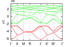
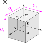
Figure 3: (a) Electron band structure corresponding to the noncoplanar magnetic order shown in Fig. 2. The Hund’s coupling is $K=t$ and superexchange constant $J=0$. (b) The reduced Brillouin zone with high-symmetry points and lines.

Fig. 3(a) shows the electron band structure corresponding to the noncoplanar magnetic order. The spectrum is at least doubly degenerate thanks to a combined lattice translation and spin rotation symmetry. Due to the nesting effect, a charge gap opens between the lower four pairs of bands and other high energy branches. It is known that the electron experiences a fictitious magnetic field proportional to the spin chirality $\chi_{ijk}=\mathbf{S}_{i}\cdot\mathbf{S}_{j}\times\mathbf{S}_{k}$ nakatsuji when hopping around a triangular loop. Although $\chi_{ijk}$ is nonzero in the noncoplanar structure, the contributions from the four triangular faces of a tetrahedron cancel each other due to a monopole-like spin configuration. The noncoplanar magnetic order thus does not exhibit a spontaneous quantum Hall effect.

The magnetic structure itself, nonetheless, breaks the chiral symmetry. This is best illustrated by projecting the triple-$\mathbf{Q}$ magnetic order onto a $(111)$ kagome plane which shows hexagons and triangles with a definite handedness [Fig. 2(b)]. More specifically, we introduce a scalar chirality for a tetrahedron in the antiferromagnetic state:

$$\chi_{\boxtimes}=3\sqrt{3}\,\,\mathbf{L}_{1}\cdot\mathbf{L}_{2}\times\mathbf{L}_{3}.$$ (12)

The noncoplanar magnetic order shown in Fig. 2 has the maximum chirality $\langle\chi_{\boxtimes}\rangle=+1$, where the average is over both types of tetrahedra. This is to be contrasted with the so called all-in all-out structure [Fig. 4(a)] in which the two types of tetrahedra have opposite chiralities $\langle\chi_{\rm I}\rangle=-\langle\chi_{\rm II}\rangle$; the average chirality is thus zero.

The model described by Eq. (1) with a negative $K$ was recently investigated in Ref. motome10, using Monte Carlo simulations. The authors also considered the special case of quarter filling. However, since the simulations were performed assuming a large Hund’s coupling, the noncoplanar magnetic order shown in Fig. 2 was not observed in their simulations. Although the fine structure of the electron Fermi surface is absent in small finite systems, the noncoplanar magnetic order could be found in Monte Carlo simulations at small Hund’s coupling using techniques such as twisted boundary conditions motome10 .

We now turn to the spin-ice compounds where the rotational symmetry is explicitly broken by a strong easy-axis anisotropy $H_{D}=-D\sum_{i}(\mathbf{S}_{i}\cdot\hat{\mathbf{e}}_{m})^{2}$. The effective degrees of freedom become discrete Ising variables as spins are forced to point along the local $\langle 111\rangle$ directions. We start with the $J=0$ limit. At filling factor $\nu=1/4$, simulated annealing yields a ground state with the all-in all-out magnetic order shown in Fig. 4(a). The fact that every tetrahedron has total spin $\mathbf{M}_{\boxtimes}=0$ makes the all-in all-out structure a simultaneous ground state of the antiferromagnetic inter-site couplings.

In spin-ice compounds, however, the nearest-neighbor exchange has a ferromagnetic sign, i.e. $J=-|J|$. Assuming $D\gg|J|\gg t$, $K$, numerical minimization gives a single-$\mathbf{Q}$ 2-in 2-out structure [Fig. 4(b)]. The magnetizations of type-I and type-II tetrahedra point along $a$ and $b$ axes, respectively, with their sign alternating between adjacent $ab$ planes. There is a total of six degenerate single-$\mathbf{Q}$ states related by time reversal and lattice translation symmetries.

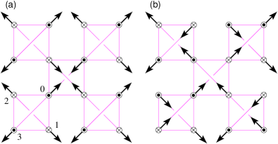
Figure 4: (a) All-in all-out structure. (b) 2-in 2-out magnetic order with wavevecotr $\mathbf{Q}_{3}=2\pi(0,0,1)$. The $\odot$ and $\otimes$ symbols again denote spin component coming out of and into the plane, respectively.

Both magnetic orders shown in Fig. 4 were obtained in a recent Monte Carlo study on a metallic pyrochlore spin ice ikeda08 . Instead of tackling the Kondo-lattice model directly, the simulations were performed assuming a long-range RKKY interaction between localized spins. Neglecting the superexchange $J$, their simulations yielded a 2-in 2-out structure at quarter filling ikeda08 , which is in disagreement with our result (the all-in all-out state). This discrepancy could be attributed to the fact that the RKKY interaction is derived by integrating out the electrons with a spherical Fermi surface. The approach thus neglects the subtle effect of Fermi surface nesting.

In summary, we have studied a model of itinerant electrons interacting with localized classical spins on the pyrochlore lattice. At quarter filling, we showed that a noncoplanar magnetic order emerges as a ground state of the rotationally invariant Hamiltonian. The magnetic structure characerized by a nozero order parameter $\chi_{\boxtimes}$ also breaks the chiral symmetry. Since the chiral transition needs not coincide with the magnetic ordering from the symmetry viewpoint, a chiral phase with $\langle\chi_{\boxtimes}\rangle\neq 0$ but no spin order $\langle\mathbf{L}_{i}\rangle=0$ could occur at finite temperatures. A similar case was recently observed in spin ice compound Pr₂Ir₂O₇ machida . Future studies, especially large-scale Monte Carlo simulations, could demonstrate the noncoplanar magnetic structure numerically and explore the possibility of the partially ordered chiral phase. Finally, we showed that when the localized spins are subject to strong uniaxial anisotropy, the on-site Hund’s coupling favors a uniform all-in all-out spin structure, whereas the single-$\mathbf{Q}$ 2-in 2-out magnetic order is stabilized by the inter-site ferromagnetic exchange interaction.

Acknowledgment. I am grateful to Y. Kato, I. Martin, Y. Motome, and N. Perkins for stimulating discussions, and especially to C.D. Batista for pointing out the logarithmic divergence of susceptibility and various invaluable comments. The author also acknowleges the support of ICAM and NSF Grant DMR-0844115.

References

- (1) R. Moessner and J. T. Chalker, Phys. Rev. Lett. 80, 2929 (1998); Phys. Rev. B 58, 12049 (1998).
- (2) S.-H. Lee et al., Phys. Rev. Lett. 84, 3718 (2000); J.-H. Chung et al., Phys. Rev. Lett. 95, 247204 (2005).
- (3) O. Tchernyshyov, R. Moessner, S. L. Sondhi, Phys. Rev. Lett. 88, 067203 (2002); Phys. Rev. B 66, 064403 (2002).
- (4) G.-W. Chern, C. Fennie, and O. Tchernyshyov, Phys. Rev. B 74, 060405(R) (2006).
- (5) S.-H. Lee et al., Phys. Rev. Lett. 93, 15640 (2004).
- (6) V. O. Garlea et al., Phys. Rev. Lett. 100, 066404 (2008).
- (7) O. Tchernyshyov, Phys. Rev. Lett. 93, 157206 (2004).
- (8) G.-W. Chern and N. Perkins, Phys. Rev. B 80, 180409(R) (2009); G.-W. Chern, N. Perkins, Z. Hao, Phys. Rev. B 81, 125127 (2010).
- (9) D. Ikoma, H. Tsuchiura, and J. Inoue, Phys. Rev. B 68, 014420 (2003).
- (10) A. Ikeda and H. Kawamura, J. Phys. Soc. Jpn. 77, 073707 (2008).
- (11) Y. Motome and N. Furukawa, Phys. Rev. Lett., 104, 106407 (2010); J. Phys. Conf. Ser. 200, 012131 (2010).
- (12) C. Lacroix, J. Phys. Soc. Jap. 79, 011008 (2010).
- (13) I. Martin and C. D. Batista, Phys. Rev. Lett., 101, 156402 (2008).
- (14) Y. Akagi and Y. Motome, J. Phys. Soc. Jpn., to be published (2010).
- (15) Y. Kato and C. D. Batista, unpublished (2010).
- (16) S. Nakatsuji et al. Phys. Rev. Lett. 96, 087204 (2006).
- (17) Y. Machida et al. Nature 463, 210 (2010).