Abstract

We present a full diagrammatic computation of the one-loop corrections from the neutrino/sneutrino sector to the renormalized neutral ${\cal CP}$-even Higgs boson self-energies and the lightest Higgs boson mass, $M_{h}$, within the context of the so-called MSSM-seesaw scenario. This consists of the Minimal Supersymmetric Standard Model with the addition of massive right handed Majorana neutrinos and their supersymmetric partners, and where the seesaw mechanism is used for the lightest neutrino mass generation. We explore the dependence on all the parameters involved, with particular emphasis in the role played by the heavy Majorana scale. We restrict ourselves to the case of one generation of neutrinos/sneutrinos. For the numerical part of the study, we consider a very wide range of values for all the parameters involved. We find sizeable corrections to $M_{h}$, which are negative in the region where the Majorana scale is large ($10^{13}-10^{15}\,\,\mathrm{GeV}$) and the lightest neutrino mass is within a range inspired by data ($0.1-1$ eV). For some regions of the MSSM-seesaw parameter space, the corrections to $M_{h}$ are substantially larger than the anticipated Large Hadron Collider precision.

1 Introduction

The current impressive experimental data on neutrino mass differences and neutrino mixing angles [1] indicate clearly a signal of new physics beyond the so far successful Standard Model of Particle Physics (SM). In order to incorporate the non-vanishing neutrino masses required by data an extension of the SM with massive neutrinos is mandatory. Among the various possibilities to extend the SM we choose here the most popular one that incorporates massive Majorana neutrinos and also stabilizes the electroweak symmetry breaking scale, $v=174\,\,\mathrm{GeV}$, against potentially large radiative corrections in the presence of the new physics scale. We refer to the simplest version of a supersymmetric extension of the SM, the Minimal Supersymmetric Standard Model (MSSM) [2], with the addition of heavy right-handed Majorana neutrinos, and where the well known seesaw mechanism of type I [3] is implemented to generate the observed small neutrino masses. From now on we will denote this model by “MSSM-seesaw”.

In this MSSM-seesaw context, the smallness of the light neutrino masses, $m_{\nu}\sim m_{D}^{2}/m_{M}$, appears naturally due to the induced large suppression by the ratio of the two very distant mass scales. Namely, the Majorana neutrino mass $m_{M}$, that represents the new physics scale, and the Dirac neutrino mass $m_{D}$, which is related to the electroweak scale via the neutrino Yukawa couplings $Y_{\nu}$, by $m_{D}=Y_{\nu}v\sin\beta$. The Higgs sector content in the MSSM-seesaw is as in the MSSM [4], and $\tan\beta$ is given, as usual, by the ratio of the two MSSM Higgs vacuum expectation values (v.e.v.s). Although the present neutrino data requires two or more neutrino generations, we shall adopt here the simplest case of one neutrino generation in order to fully understand first the role of one single Majorana scale $m_{M}$, and postpone the more complex case of three generations for a future work. In this simplified one-generation MSSM-seesaw framework, small neutrino masses of the order of $m_{\nu}\sim 0.1-1$ eV can be easily accommodated with large Yukawa couplings, $Y_{\nu}\sim{\cal O}(1)$, if the new physics scale is very large, within the range $m_{M}\sim 10^{13}-10^{15}\,\,\mathrm{GeV}$. This is to be compared with the Dirac neutrino case where, in order to get similar small neutrino masses, extremely tiny, hence irrelevant, Yukawa couplings of the order of $Y_{\nu}\sim 10^{-12}-10^{-13}$ are required.

The hypothesis of Majorana massive neutrinos is very appealing for various reasons, including the interesting possibility of generating satisfactorily baryogenesis via leptogenesis [5], and also because they can produce an interesting and singular phenomenology due to their potentially large Yukawa couplings to the Higgs sector of the theory, the MSSM in the present case. Among the most striking phenomenological implications of these MSSM-seesaw scenarios [6], it is worth mentioning: 1) the prediction of sizeable rates for lepton flavor violating processes, indeed within the present experimental reach for specific areas of the model parameters [7, 8], 2) non-negligible contributions to electric dipole moments of charged leptons [9], and 3) the occurrence of sneutrino-antisneutrino oscillations [10] and sneutrino flavor-oscillations [11].

The present paper investigates another implication of heavy Majorana neutrinos that could be as relevant as these previously mentioned ones. More specifically, we are interested here in the indirect effects of Majorana neutrinos via their radiative corrections to the MSSM Higgs boson masses. In particular, our study will be focused on the radiative corrections to the lightest MSSM ${\cal CP}$-even $h$ boson mass, $M_{h}$, due to the one-loop contributions from the neutrino/sneutrino sector within the MSSM-seesaw framework. Previous studies in particular SUSY scenarios and under specific assumptions on the model parameters [12, 13, 8, 14] indicate that the size of these radiative corrections to the Higgs mass parameters in the case of extremely heavy Majorana neutrinos can be sizeable due to the large size of $Y_{\nu}$.

For the estimates of the total corrections to $M_{h}$ in the MSSM-seesaw, obviously, the one-loop corrections from the neutrino/sneutrino sector that we are interested here have to be added to the existing MSSM corrections. The status of radiative corrections to $M_{h}$ in the non-$\nu/\tilde{\nu}$ sector, i.e. in the MSSM without massive neutrinos, can be summarized as follows. Full one-loop calculations [15] have been supplemented by the leading and subleading two-loop corrections, see [16] and references therein. Together with leading three-loop corrections [17] the current precision in $M_{h}$ is estimated to be $\sim 2-3\,\,\mathrm{GeV}$ [16].

Regarding the previous estimates of neutrino/sneutrino radiative corrections to the Higgs mass parameters the status is as follows. In Ref. [12] the one-loop corrections to $M_{h}$ were estimated within a split SUSY scenario where the soft-SUSY-breaking mass associated to the right handed neutrino, $m_{\tilde{R}}$, was chosen to be very large, of the order of the Majorana scale $m_{M}$. They worked in the zero external momentum approximation and switching off the $SU(2)\times U(1)$ gauge interactions. Besides, they used the mass insertion approximation for the other soft-breaking sneutrino parameters, $A_{\nu}$ and $B_{\nu}$, associated to the trilinear coupling and neutrino $B$-term respectively. A large and negative correction from the neutrino/sneutrino sector of the order of a few tens of GeV was found for $m_{M}=10^{14}\,\,\mathrm{GeV}$ and $m_{\tilde{R}}\sim{\cal O}(m_{M})$. In Ref. [13] the radiative one-loop effects of the neutrino $B$-term on the Higgs mass parameters within the context of mSUGRA (with universal scalar masses at the $m_{\rm SUSY}$, including $m_{\tilde{R}}$) were analyzed by means of the renormalization group equations (RGEs). They found large effects from this $B_{\nu}$ term that indeed could destabilize the electroweak symmetry breaking. By requiring a proper breaking in this mSUGRA framework they concluded with an upper bound of $B_{\nu}Y_{\nu}^{2}/(8\pi^{2})<m_{\rm SUSY}/\tan\beta$. Large corrections to the Higgs soft mass parameters within a SUSY-seesaw framework with total or partial universality conditions have also been found by a similar RGEs analysis in [8, 14]. In [8] it was concluded that these corrections induce a considerable decrease in the physical Higgs boson masses which in turn enhance the rates of the Higgs-mediated LFV processes. In [14] the large threshold corrections found from the heavy neutrinos/sneutrinos were shown to affect, and even dominate at large $B_{\nu}$, the radiative breaking of the electroweak symmetry and also modify considerably the predictions on the neutralino dark matter abundance.

In this work, we will consider instead the more general MSSM-seesaw scenarios with no universality conditions imposed, and explore the full parameter space, without restricting ourselves just to large or small values on neither of the relevant neutrino/sneutrino parameters. In principle, since the right handed Majorana neutrinos and their SUSY partners are $SU(2)\times U(1)$ singlets, there is no a priori reason why the size of their associated parameters should be related to the size of the other sector parameters. In the numerical estimates, we will therefore explore a wide interval for all the involved neutrino/sneutrino relevant input parameters.

We will present here a full one-loop computation of the radiative corrections to the lightest ${\cal CP}$-even Higgs boson mass from the (one generation) neutrino/sneutrino sector in which we will not use any of the previous approximations and we will not set the external momentum to zero. The complete set of one-loop neutrino/sneutrino contributing diagrams will be taken into account, with both Yukawa and gauge couplings switched on. We also analyze the results in several renormalization schemes, which will be shown to provide remarkable differences. In addition, we present some analytical and numerical results in the interesting limit of very large $m_{M}$ as compared to all other scales involved, which will help us in the understanding of the important issue of the decoupling/non-decoupling of the heavy Majorana scale. Our further study in the particular region of large $m_{M}$ and $m_{\tilde{R}}$ will also allow us to compare our results with those in [12].

Our final aim is to find out to what extent the radiative corrections computed here enter into the measurable range. The experimental perspectives for the Higgs mass measurements with precision enough to be sensitive to such sizeable radiative corrections, as the ones found here, are indeed quite promising. The LHC has good prospects to discover at least one neutral Higgs boson over the full MSSM parameter space and a precision on the mass of a Standard Model (SM)-like Higgs boson of $\sim 200\,\,\mathrm{MeV}$ are expected [18, 19, 20, 21] (see e.g. [22, 23] for reviews). At the ILC a determination of the Higgs boson properties (within the kinematic reach) will be possible, and an accuracy on the mass could reach the $50\,\,\mathrm{MeV}$ level [24, 25, 26, 27]. The interplay of the LHC and the ILC in the neutral MSSM Higgs sector will improve certainly these measurements [28, 29].

The paper is organized as follows. In section 2, we summarize the most important ingredients of the MSSM-seesaw scenario that are needed for the present computation of the Higgs mass loop corrections. These include, the setting of the model parameters and the complete list of the Lagrangian relevant terms. A complete set of the corresponding relevant Feynman rules in the physical basis is also provided here. They are collected in the Appendix A and, to our knowledge, they are not available in the previous literature. We also comment shortly in section 2 on the comparison between the Dirac and the Majorana cases. In section 3 we present the renormalization procedure and emphasize the differences between the selected renormalization schemes, specifically, the on-shell and the ${\overline{\mathrm{DR}}}$ schemes. Section 4 is devoted to the results. First we present the analytical results for the renormalized Higgs boson self-energies (the main formulas are collected in Appendix B). Then we present the numerical results in terms of all the relevant neutrino/sneutrino parameters that we explore exhaustively in the full plausible range. We also include in this section a study of the behavior of the renormalized Higgs self-energies in the large $m_{M}$ limit. The final part of this section summarizes the main numerical results for the lightest Higgs boson mass corrections. Finally, section 5 contains the conclusions.

2 The MSSM-seesaw model

The model we are interested in here is the MSSM extended by right handed neutrinos and their SUSY partners, and where a seesaw mechanism of type I [3] is implemented to generate the neutrino masses and mixing angles. This is called usually the MSSM-seesaw model. For simplicity, as already announced in the introduction, we will restrict here to the one generation neutrinos/sneutrinos case although the full compatibility with present neutrino data for mass differences and mixing angles, requires additional neutrino generations. Since the main idea is to analyze the radiative corrections from the neutrino-sneutrino sector to the lightest Higgs mass, we restrict ourselves to the case of one generation of neutrinos/sneutrinos. We illustrate first this simpler case and postpone the more complex case of three generations for a future work.

2.1 The neutrino/sneutrino sector

The MSSM-seesaw model with one neutrino/sneutrino generation is described in terms of the well known MSSM superpotential plus the new relevant terms contained in:

$$W\,=\,\epsilon_{ij}\left[Y_{\nu}\hat{H}_{2}^{i}\,\hat{L}^{j}\hat{N}\,-\,Y_{l}\hat{H}_{1}^{i}\,\hat{L}^{j}\,\hat{R}\right]\,+\,\frac{1}{2}\,\hat{N}\,m_{M}\,\hat{N}\,,$$ (1)

where $m_{M}$ is the Majorana mass and $\hat{N}=(\tilde{\nu}_{R}^{*},(\nu_{R})^{c})$ is the additional superfield that contains the right-handed neutrino $\nu_{R}$ and its scalar partner $\tilde{\nu}_{R}$. Here and in the following $f^{c}$ denotes the particle-antiparticle conjugate (c-conjugate in short) of a fermion $f$ ($f^{c}=C{\bar{f}}^{T}$) and $\tilde{f}^{*}$ denotes the complex conjugate of sfermion $\tilde{f}$. The lepton Yukawa couplings are $Y_{l,\nu}$, and we use the convention $\epsilon_{12}=-1$ . The other superfields, $\hat{L}$ containing the lepton ($\nu_{L},e_{L}$) and slepton ($\tilde{\nu}_{L},\tilde{e}_{L}$) $SU(2)$ doublets, $\hat{R}$ containing the lepton $(e_{R})^{c}$ and slepton $\tilde{e}_{R}^{*}$ $SU(2)$ singlets, and $\hat{H}_{1,2}$ containing the Higgs boson $SU(2)$ doublets and their SUSY partners, are as in the MSSM. We follow here the notation of  [4].

There are also new relevant terms in the soft SUSY breaking potential due to the additional sneutrinos $\tilde{\nu}_{R}$ [10]:

$$V^{\tilde{\nu}}_{\rm soft}=m^{2}_{\tilde{L}}\tilde{\nu}_{L}^{*}\tilde{\nu}_{L}+m^{2}_{\tilde{R}}\tilde{\nu}_{R}^{*}\tilde{\nu}_{R}+(Y_{\nu}A_{\nu}H^{2}_{2}\tilde{\nu}_{L}\tilde{\nu}_{R}^{*}+m_{M}B_{\nu}\tilde{\nu}_{R}\tilde{\nu}_{R}+{\rm h.c.})~{}.$$ (2)

After electro-weak (EW) symmetry breaking, the charged lepton and Dirac neutrino masses can be written as

$$m_{l}\,=\,Y_{l}\,\,v_{1}\,,\quad\quad m_{D}\,=\,Y_{\nu}\,v_{2}\,,$$ (3)

where $v_{i}$ are the vacuum expectation values (VEVs) of the neutral Higgs scalars, with $v_{1(2)}=\,v\,\cos(\sin)\beta$ and $v=174\,\,\mathrm{GeV}$.

The $2\times 2$ neutrino mass matrix is given in terms of $m_{D}$ and $m_{M}$ by:

$$M^{\nu}\,=\,\left(\begin{array}[]{cc}0&m_{D}\\ m_{D}&m_{M}\end{array}\right)\,.$$ (4)

Diagonalization of $M^{\nu}$ leads to two mass eigenstates, $n_{i}\,(i=1,2)$, which are Majorana fermions:

$$n_{1} \equiv\nu=\cos\theta(\nu_{L}+(\nu_{L})^{c})-\sin\theta(\nu_{R}+(\nu_{R})^{c})~{},$$

$$n_{2} \equiv N=\sin\theta(\nu_{L}+(\nu_{L})^{c})+\cos\theta(\nu_{R}+(\nu_{R})^{c})$$ (5)

with the respective mass eigenvalues given by:

$$m_{\nu,\,N}=\frac{1}{2}\left(m_{M}\mp\sqrt{m_{M}^{2}+4m_{D}^{2}}\right)~{}.$$ (6)

It should be noticed that we have introduced an alternative notation that makes it easier to identify the specific neutrino by its mass: $\nu$ is the lighter one and $N$ is the heavier one. It should also be kept in mind that with this convention $m_{\nu}<0$ and $m_{N}>0$, but the physical Majorana neutrino states have the proper positive masses. These physical neutrinos can be reached by an additional rotation, $\nu\to\nu^{\prime}=e^{i\gamma_{5}\pi/2}\nu=-i\gamma_{5}\nu$, leading to $m_{\nu^{\prime}}=|m_{\nu}|$. However, we prefer to work instead with the mass eigenstates in (2.1) to avoid extra $i$ and $\gamma_{5}$ factors in the computation. Of course the final results in this work for the Higgs mass corrections are not sensitive to this choice.

The mixing angle that defines the mass eigenstates is given by,

$$\tan\theta=-\frac{m_{\nu}}{m_{D}}=\frac{m_{D}}{m_{N}}~{}.$$ (7)

Other useful relations between the model parameters $m_{D}$, $m_{M}$ and the physical neutrino parameters, $m_{\nu}$, $m_{N}$ and $\theta$ are the following:

$$\sin^{2}\theta =\frac{-m_{\nu}}{m_{N}-m_{\nu}}=\frac{1}{2}\left(1-\frac{m_{M}}{\sqrt{m_{M}^{2}+4m_{D}^{2}}}\right)~{},$$ (8)

$$\cos^{2}\theta =\frac{m_{N}}{m_{N}-m_{\nu}}=\frac{1}{2}\left(1+\frac{m_{M}}{\sqrt{m_{M}^{2}+4m_{D}^{2}}}\right)~{},$$ (9)

$$m_{D} =\frac{1}{2}\sqrt{(m_{N}-m_{\nu})^{2}-(m_{N}+m_{\nu})^{2}}~{},$$ (10)

$$m_{D}^{2} =-m_{\nu}m_{N}~{},$$ (11)

$$m_{M} =m_{\nu}+m_{N}~{}.$$ (12)

Regarding the sneutrino sector, the sneutrino mass matrices for the ${\cal CP}$-even, ${\tilde{M}}_{+}$, and the ${\cal CP}$-odd, ${\tilde{M}}_{-}$, subsectors are given respectively by [10]:

$${\tilde{M}}_{\pm}^{2}=\left(\begin{array}[]{cc}m_{\tilde{L}}^{2}+m_{D}^{2}+\frac{1}{2}M_{Z}^{2}\cos 2\beta&m_{D}(A_{\nu}-\mu\cot\beta\pm m_{M})\\ m_{D}(A_{\nu}-\mu\cot\beta\pm m_{M})&m_{\tilde{R}}^{2}+m_{D}^{2}+m_{M}^{2}\pm 2B_{\nu}m_{M}\end{array}\right)~{}.$$ (13)

The diagonalization of these two matrices, ${\tilde{M}}_{\pm}^{2}$, leads to four sneutrino mass eigenstates, ${\tilde{n}}_{i}\,(i=1,2,3,4)$ with respective ${\cal CP}$ parities ${\cal CP}(\tilde{n}_{1,2})=+1$ and ${\cal CP}({\tilde{n}}_{3,4})=-1$:

$${\tilde{n}}_{1} \equiv\tilde{\nu}_{+}=\sqrt{2}(\cos\theta_{+}\mathop{\mathrm{Re}}\tilde{\nu}_{L}-\sin\theta_{+}\mathop{\mathrm{Re}}\tilde{\nu}_{R})~{},$$

$${\tilde{n}}_{2} \equiv\tilde{N}_{+}=\sqrt{2}(\sin\theta_{+}\mathop{\mathrm{Re}}\tilde{\nu}_{L}+\cos\theta_{+}\mathop{\mathrm{Re}}\tilde{\nu}_{R})~{},$$

$${\tilde{n}}_{3} \equiv\tilde{\nu}_{-}=\sqrt{2}(\cos\theta_{-}\mathop{\mathrm{Im}}\tilde{\nu}_{L}-\sin\theta_{-}\mathop{\mathrm{Im}}\tilde{\nu}_{R})~{},$$

$${\tilde{n}}_{4} \equiv\tilde{N}_{-}=\sqrt{2}(\sin\theta_{-}\mathop{\mathrm{Im}}\tilde{\nu}_{L}+\cos\theta_{-}\mathop{\mathrm{Im}}\tilde{\nu}_{R})~{}.$$ (14)

It should again be noted that we have introduced an alternative notation that makes it easier to identify the specific sneutrino by its parity and mass: $\tilde{\nu}_{+}$, $\tilde{N}_{+}$ are respectively the lighter and the heavier ones with ${\cal CP}=+1$, and $\tilde{\nu}_{-}$, $\tilde{N}_{-}$ are the lighter and the heavier ones with ${\cal CP}=-1$. The corresponding mass eigenvalues are:

$$m_{{\tilde{\nu}_{+}},{\tilde{N}_{+}}}^{2} =\frac{1}{2}(m_{M}^{2}+m_{\tilde{L}}^{2}+m_{\tilde{R}}^{2}+2m_{D}^{2}+\frac{1}{2}M_{Z}^{2}\cos 2\beta+2B_{\nu}m_{M})$$ (15)

$$\;\mp\frac{1}{2}\sqrt{4m_{D}^{2}(A_{\nu}-\mu\cot\beta+m_{M})^{2}+(m_{M}^{2}+m_{\tilde{R}}^{2}-m_{\tilde{L}}^{2}-\frac{1}{2}M_{Z}^{2}\cos 2\beta+2B_{\nu}m_{M})^{2}}~{},$$

$$m_{{\tilde{\nu}_{-}},{\tilde{N}_{-}}}^{2} =\frac{1}{2}(m_{M}^{2}+m_{\tilde{L}}^{2}+m_{\tilde{R}}^{2}+2m_{D}^{2}+\frac{1}{2}M_{Z}^{2}\cos 2\beta-2B_{\nu}m_{M})$$ (16)

$$\;\mp\frac{1}{2}\sqrt{4m_{D}^{2}(A_{\nu}-\mu\cot\beta-m_{M})^{2}+(m_{M}^{2}+m_{\tilde{R}}^{2}-m_{\tilde{L}}^{2}-\frac{1}{2}M_{Z}^{2}\cos 2\beta-2B_{\nu}m_{M})^{2}}~{}.$$

The mixing angles in the two subsectors are given respectively by:

$$\sin 2\theta_{\pm}=\frac{2m_{D}(A_{\nu}-\mu\cot\beta\pm m_{M})}{\sqrt{4m_{D}^{2}(A_{\nu}-\mu\cot\beta\pm m_{M})^{2}+(m_{M}^{2}+m_{\tilde{R}}^{2}-m_{\tilde{L}}^{2}-\frac{1}{2}M_{Z}^{2}\cos 2\beta\pm 2B_{\nu}m_{M})^{2}}}~{}.$$ (17)

2.2 The Higgs boson sector at tree-level

In this subsection we summarize the Higgs-boson sector of our model at tree-level. Contrary to the SM, in the MSSM two Higgs doublets are required. The Higgs potential [30]

$$V = m_{1}^{2}|{\cal H}_{1}|^{2}+m_{2}^{2}|{\cal H}_{2}|^{2}-m_{12}^{2}(\epsilon_{ab}{\cal H}_{1}^{a}{\cal H}_{2}^{b}+\mbox{h.c.})$$ (18)

$$+\frac{1}{8}(g^{2}+g^{\prime 2})\left[|{\cal H}_{1}|^{2}-|{\cal H}_{2}|^{2}\right]^{2}+\frac{1}{2}g^{2}|{\cal H}_{1}^{{\dagger}}{\cal H}_{2}|^{2}~{},$$

contains $m_{1},m_{2},m_{12}$ as soft SUSY breaking parameters; $g,g^{\prime}$ are the $SU(2)$ and $U(1)$ gauge couplings, and $\epsilon_{12}=-1$.

The doublet fields $H_{1}$ and $H_{2}$ are decomposed in the following way:

$${\cal H}_{1} = \left(\begin{array}[]{c}{\cal H}_{1}^{0}\\[2.15277pt] {\cal H}_{1}^{-}\end{array}\right)\;=\;\left(\begin{array}[]{c}v_{1}+\frac{1}{\sqrt{2}}(\phi_{1}^{0}-i\chi_{1}^{0})\\[2.15277pt] -\phi_{1}^{-}\end{array}\right)~{},$$ (23)

$${\cal H}_{2} = \left(\begin{array}[]{c}{\cal H}_{2}^{+}\\[2.15277pt] {\cal H}_{2}^{0}\end{array}\right)\;=\;\left(\begin{array}[]{c}\phi_{2}^{+}\\[2.15277pt] v_{2}+\frac{1}{\sqrt{2}}(\phi_{2}^{0}+i\chi_{2}^{0})\end{array}\right)~{}.$$ (28)

The potential (18) can be described with the help of two independent parameters (besides $g$ and $g^{\prime}$): $\tan\beta=v_{2}/v_{1}$ and $M_{A}^{2}=-m_{12}^{2}(\tan\beta+\cot\beta)$, where $M_{A}$ is the mass of the ${\cal CP}$-odd Higgs boson $A$.

The diagonalization of the bilinear part of the Higgs potential, i.e. of the Higgs mass matrices, is performed via the orthogonal transformations

$$\left(\begin{array}[]{c}H\\[2.15277pt] h\end{array}\right) = \left(\begin{array}[]{cc}\cos\alpha&\sin\alpha\\[2.15277pt] -\sin\alpha&\cos\alpha\end{array}\right)\left(\begin{array}[]{c}\phi_{1}^{0}\\[2.15277pt] \phi_{2}^{0}\end{array}\right)~{},$$ (35)

$$\left(\begin{array}[]{c}G\\[2.15277pt] A\end{array}\right) = \left(\begin{array}[]{cc}\cos\beta&\sin\beta\\[2.15277pt] -\sin\beta&\cos\beta\end{array}\right)\left(\begin{array}[]{c}\chi_{1}^{0}\\[2.15277pt] \chi_{2}^{0}\end{array}\right)~{},$$ (42)

$$\left(\begin{array}[]{c}G^{\pm}\\[2.15277pt] H^{\pm}\end{array}\right) = \left(\begin{array}[]{cc}\cos\beta&\sin\beta\\[2.15277pt] -\sin\beta&\cos\beta\end{array}\right)\left(\begin{array}[]{c}\phi_{1}^{\pm}\\[2.15277pt] \phi_{2}^{\pm}\end{array}\right)~{}.$$ (49)

The mixing angle $\alpha$ is determined through

$$\alpha={\rm arctan}\left[\frac{-(M_{A}^{2}+M_{Z}^{2})\sin\beta\cos\beta}{M_{Z}^{2}\cos^{2}\beta+M_{A}^{2}\sin^{2}\beta-m^{2}_{h}}\right]~{},~{}~{}-\frac{\pi}{2}<\alpha<0~{}.$$ (50)

One gets the following Higgs spectrum:

$$\mbox{2 neutral bosons},\,{\cal CP}=+1 : h,H$$

$$\mbox{1 neutral boson},\,{\cal CP}=-1 : A$$

2 charged bosons $$: H^{+},H^{-}$$

3 unphysical Goldstone bosons $$: G,G^{+},G^{-}.$$ (51)

At tree level the mass matrix of the neutral ${\cal CP}$-even Higgs bosons is given in the $\phi_{1}$-$\phi_{2}$-basis in terms of $M_{Z}$, $M_{A}$, and $\tan\beta$ by

$$M_{\rm Higgs}^{2} = \left(\begin{array}[]{cc}m_{\phi_{1}}^{2}&m_{\phi_{1}\phi_{2}}^{2}\\ m_{\phi_{1}\phi_{2}}^{2}&m_{\phi_{2}}^{2}\end{array}\right)$$ (54)

$$= \left(\begin{array}[]{cc}M_{A}^{2}\sin^{2}\beta+M_{Z}^{2}\cos^{2}\beta&-(M_{A}^{2}+M_{Z}^{2})\sin\beta\cos\beta\\ -(M_{A}^{2}+M_{Z}^{2})\sin\beta\cos\beta&M_{A}^{2}\cos^{2}\beta+M_{Z}^{2}\sin^{2}\beta\end{array}\right),$$ (57)

which by diagonalization according to (35) yields the tree-level Higgs boson masses

$$m_{H,h}^{2}=\frac{1}{2}\left[M_{A}^{2}+M_{Z}^{2}\pm\sqrt{(M_{A}^{2}+M_{Z}^{2})^{2}-4M_{Z}^{2}M_{A}^{2}\cos^{2}2\beta}\right]~{}.$$ (58)

The charged Higgs boson mass is given by

$$m_{H^{\pm}}^{2}=M_{A}^{2}+M_{W}^{2}~{}.$$ (59)

The masses of the gauge bosons are given in analogy to the SM:

$$M_{W}^{2}=\frac{1}{2}g^{2}(v_{1}^{2}+v_{2}^{2});\qquad M_{Z}^{2}=\frac{1}{2}(g^{2}+g^{\prime 2})(v_{1}^{2}+v_{2}^{2});\qquad M_{\gamma}=0.$$ (60)

2.3 The interaction Lagrangian

Finally the interaction Lagrangian that is relevant for the present work, expressed in the ($\nu_{L},\nu_{R}$), ($\tilde{\nu}_{L},\tilde{\nu}_{R}$) electroweak interaction basis, is given by:

$${\cal L}_{\rm int}={\cal L}_{\nu\,H}+{\cal L}_{\nu\,Z}+{\cal L}_{\tilde{\nu}\,H}+{\cal L}_{\tilde{\nu}\,Z}~{}.$$ (61)

Here ${\cal L}_{\nu\,H}$ and ${\cal L}_{\tilde{\nu}\,H}$ contain the interactions of the neutrinos and sneutrinos with the Higgs bosons respectively; and ${\cal L}_{\nu\,Z}$ and ${\cal L}_{\tilde{\nu}\,Z}$ those of the neutrinos and sneutrinos with the $Z$ boson respectively.

For the various terms in (61) we find the following expressions:

$${\cal L}_{\nu\,H} =-\frac{gm_{D}}{2M_{W}\sin\beta}((\overline{\nu_{L}}\nu_{R}+\overline{\nu_{R}}\nu_{L})(H\sin\alpha+h\cos\alpha)-i(\overline{\nu_{L}}\nu_{R}-\overline{\nu_{R}}\nu_{L})A\cos\beta)~{},$$ (62)

$${\cal L}_{\nu\,Z} =\frac{g}{2\cos\theta_{W}}\left[(\overline{\nu_{L}}\gamma^{\mu}\nu_{L})Z_{\mu}\right]~{},$$ (63)

$${\cal L}_{\tilde{\nu}\,H} =-\frac{gm_{D}}{2M_{W}\sin\beta}\mu\left[(\tilde{\nu}_{L}^{*}\tilde{\nu}_{R}+\tilde{\nu}_{L}\tilde{\nu}_{R}^{*})(-H\cos\alpha+h\sin\alpha)\right]$$

$$\quad-\frac{gm_{D}^{2}}{M_{W}\sin\beta}\left[(\tilde{\nu}_{R}^{*}\tilde{\nu}_{R}+\tilde{\nu}_{L}^{*}\tilde{\nu}_{L})(H\sin\alpha+h\cos\alpha)\right]$$

$$\quad+\frac{igm_{D}}{2M_{W}}\mu\left[(\tilde{\nu}_{L}^{*}\tilde{\nu}_{R}-\tilde{\nu}_{L}\tilde{\nu}_{R}^{*})A\right]$$

$$\quad-\frac{gM_{Z}}{2cos\theta_{W}}\left[(\tilde{\nu}_{L}^{*}\tilde{\nu}_{L})(H\cos(\alpha+\beta)-h\sin(\alpha+\beta))\right]$$

$$\quad-\frac{gm_{D}}{2M_{W}\sin\beta}A_{\nu}\left[(\tilde{\nu}_{L}^{*}\tilde{\nu}_{R}+\tilde{\nu}_{L}\tilde{\nu}_{R}^{*})(H\sin\alpha+h\cos\alpha)\right]$$

$$\quad+\frac{igm_{D}}{2M_{W}\sin\beta}A_{\nu}\left[(\tilde{\nu}_{L}^{*}\tilde{\nu}_{R}-\tilde{\nu}_{L}\tilde{\nu}_{R}^{*})A\cos\beta\right]$$

$$\quad-\frac{gm_{D}m_{M}}{2M_{W}\sin\beta}\left[(\tilde{\nu}_{L}\tilde{\nu}_{R}+\tilde{\nu}_{L}^{*}\tilde{\nu}_{R}^{*})(H\sin\alpha+h\cos\alpha)\right]$$

$$\quad-i\frac{gm_{D}m_{M}}{2M_{W}\sin\beta}\left[(\tilde{\nu}_{L}\tilde{\nu}_{R}-\tilde{\nu}_{L}^{*}\tilde{\nu}_{R}^{*})A\cos\beta\right]$$

$$\quad-\frac{g^{2}m_{D}^{2}}{4M_{W}^{2}\sin^{2}\beta}\left[(\tilde{\nu}_{L}^{*}\tilde{\nu}_{L})(H^{2}\sin^{2}\alpha+h^{2}\cos^{2}\alpha+A^{2}\cos^{2}\beta+hH\sin 2\alpha)\right]$$

$$\quad-\frac{g^{2}}{8\cos^{2}\theta_{W}}\left[(\tilde{\nu}_{L}^{*}\tilde{\nu}_{L})(H^{2}\cos 2\alpha-h^{2}\cos 2\alpha-A^{2}\cos 2\beta-2hH\sin 2\alpha)\right]$$

$$\quad-\frac{g^{2}m_{D}^{2}}{4M_{W}^{2}\sin^{2}\beta}\left[(\tilde{\nu}_{R}^{*}\tilde{\nu}_{R})(H^{2}\sin^{2}\alpha+h^{2}\cos^{2}\alpha+A^{2}\cos^{2}\beta+hH\sin 2\alpha)\right]~{},$$ (64)

$${\cal L}_{\tilde{\nu}\,Z} =-\frac{ig}{2\cos\theta_{W}}\left[(\tilde{\nu}_{L}^{*}\overleftrightarrow{\partial}^{\mu}\,\tilde{\nu}_{L})Z_{\mu}\right]+\frac{g^{2}}{4\cos^{2}\theta_{W}}\left[(\tilde{\nu}_{L}^{*}\tilde{\nu}_{L})(Z_{\mu}Z^{\mu})\right]~{}.$$ (65)

The corresponding Feynman rules, expressed in the mass eigenstate basis, are collected in the Appendix A. Notice that this complete set of Feynman rules is, to our knowledge, not available in the literature so far.

Some comments are in order. In the previous interaction Lagrangian, and consequently in the Feynman rules, there are terms already present in the MSSM. These are the pure gauge interactions between the left-handed neutrinos and the $Z$ boson, given in (63), those between the ’left-handed’ sneutrinos and the Higgs bosons, given in (2.3), and those between the ’left-handed’ sneutrinos and the $Z$ bosons, given in (65). In addition, in this MSSM-seesaw scenario, there are interactions driven by the neutrino Yukawa couplings (or equivalently $m_{D}$ since $Y_{\nu}=(gm_{D})/(\sqrt{2}M_{W}\sin\beta)$), and new interactions due to the Majorana nature driven by $m_{M}$. These genuine Majorana terms are those in the seventh and eight lines of (2.3) and are not present in the case of Dirac fermions.

2.4 Parameters and limits

Regarding the size of the new parameters that have been introduced in this model, in addition to those of the MSSM, i.e., $m_{M}$, $m_{D}$, $m_{\tilde{R}}$, $A_{\nu}$ and $B_{\nu}$, there are no significant constraints. In the literature it is often assumed that $m_{M}$ has a very large value, $m_{M}\sim{\cal O}(10^{14-15})\,\,\mathrm{GeV}$, in order to get small physical neutrino masses $|m_{\nu}|\sim$ 0.1 - 1 eV with large Yukawa couplings $Y_{\nu}\sim{\cal O}(1)$. This is an interesting possibility since it can lead to important phenomenological implications due to the large size of the radiative corrections driven by these large Yukawa couplings. In this paper we will explore, however, not only these extreme values but the full range for $m_{M}$ from the electroweak scale $\sim 10^{2}\,\,\mathrm{GeV}$ up to $\sim 10^{15}\,\,\mathrm{GeV}$.

On the other hand, the new soft SUSY-breaking parameters introduced in the sneutrino sector could be unrelated to those of the MSSM, or could be related, for instance, in the case one imposes (by hand) some kind of universality conditions. Whereas the non-singlet soft mass parameter $m_{\tilde{L}}$, being common to the charged ’left handed’ slepton, is constrained by the solution to the hierarchy problem to lie below a few TeV, the singlet soft mass $m_{\tilde{R}}$ is not, because it is not connected to the electroweak symmetry breaking at tree level. The other sneutrino soft mass parameters, $B_{\nu}$ and $A_{\nu}$ are not connected either. However, they can generate a mass-splitting between sneutrinos and antisneutrinos which in turn and via loop corrections can generate neutrino mass splittings [11] that are experimentally constrained. Then, if $m_{\rm SUSY}$ represents a generic low SUSY breaking scale, with $m_{\rm SUSY}\;\raisebox{-3.00003pt}{$\stackrel{{\scriptstyle\displaystyle<}}{{\sim}}$}\;{\cal O}(10^{3})\,\,\mathrm{GeV}$ one expects that $|A_{\nu}|,|B_{\nu}|\;\raisebox{-3.00003pt}{$\stackrel{{\scriptstyle\displaystyle<}}{{\sim}}$}\;m_{\rm SUSY}$ [13]. According to these constraints, we will explore in this work values of these soft parameters ranging from the electroweak scale up to a few TeV. Besides, and due to the peculiarity of the behavior with $m_{\tilde{R}}$ and $B_{\nu}$, as will be shown later, we will explore in addition the less conservative but interesting possibility where $m_{\tilde{R}}$ or $B_{\nu}$ are close to $m_{M}$.

For illustrative purposes and a clear understanding of our full one-loop results, three interesting limiting cases will also be considered in this work.

• The seesaw limit:
  This assumes a large separation between the two neutrino mass scales involved, the Majorana mass and the Dirac mass, $m_{M}\gg m_{D}$. Notice that both masses are different from zero, $m_{M}\neq 0$ and $m_{D}\neq 0$, in this seesaw limit and, as we have said above, $Y_{\nu}$ can be large. The predictions are then given in power series of a dimensionless parameter defined as,

  $$\xi \equiv\frac{m_{D}}{m_{M}}\ll 1~{}.$$ (66)

  The light and heavy neutrino masses are given in this limit by:

  $$m_{\nu} =-m_{D}\xi+\mathcal{O}(m_{D}\xi^{3})\simeq-\frac{m_{D}^{2}}{m_{M}}~{},$$ (67)

  $$m_{N} =m_{M}+\mathcal{O}(m_{D}\xi)\simeq m_{M}~{}.$$

  Furthermore, the mixing angle $\theta$ is small in this limit and, therefore, $\nu$ is made predominantly of $\nu_{L}$ and its c-conjugate, $(\nu_{L})^{c}$, whereas $N$ is made predominantly of $\nu_{R}$ and its c-conjugate, $(\nu_{R})^{c}$.

  In the sneutrino sector several mass scales are involved. Consequently, one has to set as an extra input their relative size to $m_{M}$. The simplest assumption is to set the value of $m_{M}$ to be much larger than all the other mass scales involved, i.e., $m_{M}\gg m_{D},M_{Z},\mu,m_{\tilde{L}},m_{\tilde{R}},B_{\nu},A_{\nu}$. In this limit the sneutrino masses are given by:

  $$m_{{\tilde{\nu}_{+}},{\tilde{\nu}_{-}}}^{2} = m_{\tilde{L}}^{2}+\frac{1}{2}M_{Z}^{2}\cos 2\beta\mp 2m_{D}(A_{\nu}-\mu\cot\beta-B_{\nu})\xi~{},$$

  $$m_{{\tilde{N}_{+}},{\tilde{N}_{-}}}^{2} = m_{M}^{2}\pm 2B_{\nu}m_{M}+m_{\tilde{R}}^{2}+2m_{D}^{2}~{}.$$ (68)

  The mixing angles $\theta_{\pm}$ are small in this limit and, therefore, ${\tilde{\nu}_{+}}$ and ${\tilde{\nu}_{-}}$ are made predominantly of ${\tilde{\nu}_{L}}$ and its c-conjugate, ${\tilde{\nu}_{L}}^{*}$, whereas ${\tilde{N}_{+}}$ and ${\tilde{N}_{-}}$ are made predominantly of ${\tilde{\nu}_{R}}$ and its c-conjugate, ${\tilde{\nu}_{R}}^{*}$.

• The Dirac limit:
  In this limit one sets $m_{M}=0$ (and $m_{D}\neq 0$) and one recovers the neutrinos as any other fermion of the MSSM, i.e., as Dirac fermions. In the basis that we have used in (2.1) this is manifested by the fact that when $m_{M}=0$, the two Majorana neutrinos $\nu$ and $N$ are degenerate with $m_{\nu}=-m_{D}$ and $m_{N}=+m_{D}$, and they combine maximally, i.e. with $\theta=\pi/4$, to form a four component Dirac neutrino with mass $m_{D}$. On the other hand, the sneutrino sector in this Dirac limit simplifies as well. When $m_{M}=0$, the real scalar fields get degenerate in pairs,

  $$m_{{\tilde{\nu}_{+}}}^{2} =m_{{\tilde{\nu}_{-}}}^{2}=\frac{1}{2}(m_{\tilde{L}}^{2}+m_{\tilde{R}}^{2}+2m_{D}^{2}+\frac{1}{2}M_{Z}^{2}\cos 2\beta)$$ (69)

  $$\quad-\frac{1}{2}\sqrt{4m_{D}^{2}(A_{\nu}-\mu\cot\beta)^{2}+(m_{\tilde{R}}^{2}-m_{\tilde{L}}^{2}-\frac{1}{2}M_{Z}^{2}\cos 2\beta)^{2}}~{},$$

  $$m_{{\tilde{N}_{+}}}^{2} =m_{{\tilde{N}_{-}}}^{2}=\frac{1}{2}(m_{\tilde{L}}^{2}+m_{\tilde{R}}^{2}+2m_{D}^{2}+\frac{1}{2}M_{Z}^{2}\cos 2\beta)$$ (70)

  $$\quad+\frac{1}{2}\sqrt{4m_{D}^{2}(A_{\nu}-\mu\cot\beta)^{2}+(m_{\tilde{R}}^{2}-m_{\tilde{L}}^{2}-\frac{1}{2}M_{Z}^{2}\cos 2\beta)^{2}}~{},$$

  and they combine to form two complex scalar fields,

  $${\tilde{\nu}}_{1} =\frac{1}{\sqrt{2}}({\tilde{\nu}_{+}}+i{\tilde{\nu}_{-}})=\cos{\tilde{\theta}}\,\,{\tilde{\nu}_{L}}-\sin{\tilde{\theta}}\,\,{\tilde{\nu}_{R}}~{},$$ (71)

  $${\tilde{\nu}}_{2} =\frac{1}{\sqrt{2}}({\tilde{N}_{+}}+i{\tilde{N}_{-}})=\sin{\tilde{\theta}}\,\,{\tilde{\nu}_{L}}+\cos{\tilde{\theta}}\,\,{\tilde{\nu}_{R}}$$ (72)

  with $m_{{\tilde{\nu}}_{1}}=m_{{\tilde{\nu}_{\pm}}}$, $m_{{\tilde{\nu}}_{2}}=m_{{\tilde{N}_{\pm}}}$, ${\tilde{\theta}}=\theta_{+}=\theta_{-}$, and

  $$\sin 2{\tilde{\theta}}=\frac{2m_{D}(A_{\nu}-\mu\cot\beta)}{\sqrt{4m_{D}^{2}(A_{\nu}-\mu\cot\beta)^{2}+(m_{\tilde{R}}^{2}-m_{\tilde{L}}^{2}-\frac{1}{2}M_{Z}^{2}\cos 2\beta)^{2}}}~{}.$$ (73)

  Notice that these two sneutrino states, ${\tilde{\nu}}_{1,2}$, are equivalent to the usual sfermion mass eigenstates within the MSSM.

  In this Dirac limit it is interesting to study the similarities in the analytical behavior of the neutrino/sneutrino radiative corrections and the other MSSM fermion/sfermion radiative corrections. In particular we are interested in the comparison with the top/stop radiative corrections. As for the phenomenological implications, this limit is not expected to lead to relevant numerical results, since to get compatibility with the experimentally tested small neutrino masses, $|m_{\nu}|\sim 0.1-1$ eV one needs Yukawa couplings extremely small, $Y_{\nu}\sim 10^{-12}-10^{-13}$.

• The MSSM limit:
  This limit is reached when one sets $m_{D}=0$ (the value of $m_{M}$ is not relevant since once the Yukawa couplings are set to zero the predictions are absolutely independent of this mass scale) and one is left with a neutrino/sneutrino sector with just pure gauge couplings. Concretely, there are just interactions of the left-handed neutrinos and the ’left-handed’ sneutrinos to the $Z$ boson, exactly as in the MSSM. We are interested in this limit, because we want to compare the radiative corrections from the neutrino/sneutrino sector within the MSSM-seesaw with those within the MSSM and to find the interesting regions in the new parameters of the MSSM-seesaw where the deviation from the MSSM result could be sizeable.

3 Higher-order corrections to $m_{h}$

3.1 The concept of higher order corrections in the
Feynman-diagrammatic approach

In the Feynman diagrammatic (FD) approach the higher-order corrected ${\cal CP}$-even Higgs boson masses in the MSSM, denoted here as $M_{h}$ and $M_{H}$ (the corresponding masses in the MSSM-seesaw model are denoted as $M_{h}^{\nu/\tilde{\nu}}$ and $M_{H}^{\nu/\tilde{\nu}}$), are derived by finding the poles of the $(h,H)$-propagator matrix. The inverse of this matrix is given by

$$\left(\Delta_{\rm Higgs}\right)^{-1}=-i\left(\begin{array}[]{cc}p^{2}-m_{H}^{2}+\hat{\Sigma}_{HH}(p^{2})&\hat{\Sigma}_{hH}(p^{2})\\ \hat{\Sigma}_{hH}(p^{2})&p^{2}-m_{h}^{2}+\hat{\Sigma}_{hh}(p^{2})\end{array}\right)~{}.$$ (74)

Determining the poles of the matrix $\Delta_{\rm Higgs}$ in (74) is equivalent to solving the equation

$$\left[p^{2}-m_{h}^{2}+\hat{\Sigma}_{hh}(p^{2})\right]\left[p^{2}-m_{H}^{2}+\hat{\Sigma}_{HH}(p^{2})\right]-\left[\hat{\Sigma}_{hH}(p^{2})\right]^{2}=0\,.$$ (75)

In perturbation theory, a (renormalized) self-energy is expanded as follows

$$\hat{\Sigma}(p^{2}) =\hat{\Sigma}^{(1)}(p^{2})+\hat{\Sigma}^{(2)}(p^{2})+\ldots~{},$$

$$\Sigma(p^{2}) =\Sigma^{(1)}(p^{2})+\Sigma^{(2)}(p^{2})+\ldots~{},$$ (76)

in terms of the $i$th-order contributions $\hat{\Sigma}^{(i)},\Sigma^{(i)}$. In the following sections we concentrate on the one-loop corrections and drop the order index, i.e. $\hat{\Sigma}\equiv\hat{\Sigma}^{(1)}$ in the following.

3.2 One-loop renormalization

In order to calculate one-loop corrections to the Higgs boson masses, the renormalized Higgs boson self-energies are needed. Here we follow the procedure used in [15, 33] (and references therein) and review it for completeness. The parameters appearing in the Higgs potential, (18), are renormalized as follows:

$$M_{Z}^{2} \to M_{Z}^{2}+\delta M_{Z}^{2}, T_{h} \to T_{h}+\delta T_{h},$$ (77)

$$M_{W}^{2} \to M_{W}^{2}+\delta M_{W}^{2}, T_{H} \to T_{H}+\delta T_{H},$$

$$M_{\rm Higgs}^{2} \to M_{\rm Higgs}^{2}+\delta M_{\rm Higgs}^{2}, \tan\beta\, \to\tan\beta\,(1+\delta\!\tan\!\beta\,).$$

$M_{\rm Higgs}^{2}$ denotes the tree-level Higgs boson mass matrix given in (57). $T_{h}$ and $T_{H}$ are the tree-level tadpoles, i.e. the terms linear in $h$ and $H$ in the Higgs potential.

The field renormalization matrices of both Higgs multiplets can be set up symmetrically,

$$\begin{pmatrix}h\\[5.0pt] H\end{pmatrix}\to\begin{pmatrix}1+\tfrac{1}{2}\delta Z_{hh}&\tfrac{1}{2}\delta Z_{hH}\\[5.0pt] \tfrac{1}{2}\delta Z_{hH}&1+\tfrac{1}{2}\delta Z_{HH}\end{pmatrix}\cdot\begin{pmatrix}h\\[5.0pt] H\end{pmatrix}~{}.$$ (78)

For the mass counter term matrices we use the definitions

$$\delta M_{\rm Higgs}^{2}=\begin{pmatrix}\delta m_{h}^{2}&\delta m_{hH}^{2}\\[5.0pt] \delta m_{hH}^{2}&\delta m_{H}^{2}\end{pmatrix}~{}.$$ (79)

The renormalized self-energies, $\hat{\Sigma}(p^{2})$, can now be expressed through the unrenormalized self-energies, $\Sigma(p^{2})$, the field renormalization constants and the mass counter terms. This reads for the ${\cal CP}$-even part,

$$\hat{\Sigma}_{hh}(p^{2}) =\Sigma_{hh}(p^{2})+\delta Z_{hh}(p^{2}-m_{h}^{2})-\delta m_{h}^{2},$$ (80a)

$$\hat{\Sigma}_{hH}(p^{2}) =\Sigma_{hH}(p^{2})+\delta Z_{hH}(p^{2}-\tfrac{1}{2}(m_{h}^{2}+m_{H}^{2}))-\delta m_{hH}^{2},$$ (80b)

$$\hat{\Sigma}_{HH}(p^{2}) =\Sigma_{HH}(p^{2})+\delta Z_{HH}(p^{2}-m_{H}^{2})-\delta m_{H}^{2}~{}.$$ (80c)

Inserting the renormalization transformation into the Higgs mass terms leads to expressions for their counter terms which consequently depend on the other counter terms introduced in (77).

For the ${\cal CP}$-even part of the Higgs sectors, these counter terms are:

$$\delta m_{h}^{2} =\delta M_{A}^{2}\cos^{2}(\alpha-\beta)+\delta M_{Z}^{2}\sin^{2}(\alpha+\beta)$$ (81a)

$$\quad+\tfrac{e}{2M_{Z}s_{\mathrm{w}}c_{\mathrm{w}}}(\delta T_{H}\cos(\alpha-\beta)\sin^{2}(\alpha-\beta)+\delta T_{h}\sin(\alpha-\beta)(1+\cos^{2}(\alpha-\beta)))$$

$$\quad+\delta\!\tan\!\beta\,\sin\beta\,\cos\beta\,(M_{A}^{2}\sin 2(\alpha-\beta)+M_{Z}^{2}\sin 2(\alpha+\beta)),$$

$$\delta m_{hH}^{2} =\tfrac{1}{2}(\delta M_{A}^{2}\sin 2(\alpha-\beta)-\delta M_{Z}^{2}\sin 2(\alpha+\beta))$$ (81b)

$$\quad+\tfrac{e}{2M_{Z}s_{\mathrm{w}}c_{\mathrm{w}}}(\delta T_{H}\sin^{3}(\alpha-\beta)-\delta T_{h}\cos^{3}(\alpha-\beta))$$

$$\quad-\delta\!\tan\!\beta\,\sin\beta\,\cos\beta\,(M_{A}^{2}\cos 2(\alpha-\beta)+M_{Z}^{2}\cos 2(\alpha+\beta)),$$

$$\delta m_{H}^{2} =\delta M_{A}^{2}\sin^{2}(\alpha-\beta)+\delta M_{Z}^{2}\cos^{2}(\alpha+\beta)$$ (81c)

$$\quad-\tfrac{e}{2M_{Z}s_{\mathrm{w}}c_{\mathrm{w}}}(\delta T_{H}\cos(\alpha-\beta)(1+\sin^{2}(\alpha-\beta))+\delta T_{h}\sin(\alpha-\beta)\cos^{2}(\alpha-\beta))$$

$$\quad-\delta\!\tan\!\beta\,\sin\beta\,\cos\beta\,(M_{A}^{2}\sin 2(\alpha-\beta)+M_{Z}^{2}\sin 2(\alpha+\beta))~{}.$$

For the field renormalization we choose to give each Higgs doublet one renormalization constant,

$${\cal H}_{1}\to(1+\tfrac{1}{2}\delta Z_{{\cal H}_{1}}){\cal H}_{1},\quad{\cal H}_{2}\to(1+\tfrac{1}{2}\delta Z_{{\cal H}_{2}}){\cal H}_{2}~{}.$$ (82)

This leads to the following expressions for the various field renormalization constants in (78):

$$\delta Z_{hh} =\sin^{2}\!\alpha\,\delta Z_{{\cal H}_{1}}+\cos^{2}\!\alpha\,\delta Z_{{\cal H}_{2}},$$ (83a)

$$\delta Z_{hH} =\sin\alpha\,\cos\alpha\,(\delta Z_{{\cal H}_{2}}-\delta Z_{{\cal H}_{1}}),$$ (83b)

$$\delta Z_{HH} =\cos^{2}\!\alpha\,\delta Z_{{\cal H}_{1}}+\sin^{2}\!\alpha\,\delta Z_{{\cal H}_{2}}~{}.$$ (83c)

The counter term for $\tan\beta$ can be expressed in terms of the vacuum expectation values as

$$\delta\tan\beta=\frac{1}{2}\left(\delta Z_{{\cal H}_{2}}-\delta Z_{{\cal H}_{1}}\right)+\frac{\delta v_{2}}{v_{2}}-\frac{\delta v_{1}}{v_{1}}~{},$$ (84)

where the $\delta v_{i}$ are the renormalization constants of the $v_{i}$:

$$v_{1}\to\left(1+\delta Z_{{\cal H}_{1}}\right)\left(v_{1}+\delta v_{1}\right),\quad v_{2}\to\left(1+\delta Z_{{\cal H}_{2}}\right)\left(v_{2}+\delta v_{2}\right)~{}.$$ (85)

It can be shown that the divergent parts of $\delta v_{1}/v_{1}$ and $\delta v_{2}/v_{2}$ are equal [15]. Consequently, one can set $\delta v_{2}/v_{2}-\delta v_{1}/v_{1}$ to zero.

The renormalization conditions are fixed by an appropriate renormalization scheme. For the mass counter terms on-shell conditions are used, leading to:

$$\delta M_{Z}^{2}=\mathop{\mathrm{Re}}\Sigma_{ZZ}(M_{Z}^{2}),\quad\delta M_{W}^{2}=\mathop{\mathrm{Re}}\Sigma_{WW}(M_{W}^{2}),\quad\delta M_{A}^{2}=\mathop{\mathrm{Re}}\Sigma_{AA}(M_{A}^{2}).$$ (86)

Here $\Sigma_{ZZ,WW}$ denotes the transverse part of the self-energies. Since the tadpole coefficients are chosen to vanish in all orders, their counter terms follow from $T_{\{h,H\}}+\delta T_{\{h,H\}}=0$:

$$\delta T_{h}=-{T_{h}},\quad\delta T_{H}=-{T_{H}}~{}.$$ (87)

For the remaining renormalization constants for $\delta\tan\beta$, $\delta Z_{{\cal H}_{1}}$ and $\delta Z_{{\cal H}_{2}}$ various renormalization schemes are possible [31, 32, 33].

On-shell renormalization

One possible choice is an on-shell (OS) renormalization. The renormalization conditions for the renormalized Higgs-boson self-energies are

$$\hat{\Sigma}^{\prime}_{hh}(m_{h}^{2}) =0~{},$$ (88)

$$\hat{\Sigma}^{\prime}_{HH}(m_{H}^{2}) =0~{}.$$ (89)

This yields

$$\delta Z_{hh}^{\mathrm{OS}} =-\mathop{\mathrm{Re}}\Sigma^{\prime}_{hh}(m_{h}^{2})~{},$$ (90)

$$\delta Z_{HH}^{\mathrm{OS}} =-\mathop{\mathrm{Re}}\Sigma^{\prime}_{HH}(m_{H}^{2})~{},$$ (91)

equivalently to

$$\delta Z_{{\cal H}_{1}}^{\mathrm{OS}} =\frac{1}{\cos 2\alpha}\left(\sin^{2}\!\alpha\,\mathop{\mathrm{Re}}\Sigma^{\prime}_{hh}(m_{h}^{2})-\cos^{2}\!\alpha\,\mathop{\mathrm{Re}}\Sigma^{\prime}_{HH}(m_{H}^{2})\right)~{},$$ (92)

$$\delta Z_{{\cal H}_{2}}^{\mathrm{OS}} =\frac{1}{\cos 2\alpha}\left(-\cos^{2}\!\alpha\,\mathop{\mathrm{Re}}\Sigma^{\prime}_{hh}(m_{h}^{2})+\sin^{2}\!\alpha\,\mathop{\mathrm{Re}}\Sigma^{\prime}_{HH}(m_{H}^{2})\right)~{}.$$ (93)

For $\delta\tan\beta^{\mathrm{OS}}$ a convenient choice is

$$\delta\tan\beta^{\mathrm{OS}} =\frac{1}{2}\left(\delta Z_{{\cal H}_{2}}^{\mathrm{OS}}-\delta Z_{{\cal H}_{1}}^{\mathrm{OS}}\right)$$

$$=\frac{-1}{2\cos 2\alpha}\left(\mathop{\mathrm{Re}}\Sigma^{\prime}_{hh}(m_{h}^{2})-\mathop{\mathrm{Re}}\Sigma^{\prime}_{HH}(m_{H}^{2})\right)~{}.$$ (94)

It should be kept in mind that this scheme can lead to large corrections to $m_{h}$ in the MSSM [31, 34], hence worsening the convergence of the perturbative expansion. Furthermore, it is known to provide gauge dependent corrections at the one-loop level [32].

$\overline{\mathrm{DR}}$ renormalization

A convenient choice which avoids the previously commented large corrections to $m_{h}$ in the MSSM and is (linear) gauge independent at the one-loop level is a $\overline{\rm{DR}}$ renormalization of $\delta\tan\beta$, $\delta Z_{{\cal H}_{1}}$ and $\delta Z_{{\cal H}_{2}}$,

$$\delta Z_{{\cal H}_{1}}^{\overline{\mathrm{DR}}} =-\left[\mathop{\mathrm{Re}}\Sigma^{\prime}_{HH\;|\alpha=0}\right]^{\rm div},$$ (95a)

$$\delta Z_{{\cal H}_{2}}^{\overline{\mathrm{DR}}} =-\left[\mathop{\mathrm{Re}}\Sigma^{\prime}_{hh\;|\alpha=0}\right]^{\rm div},$$ (95b)

$$\delta\!\tan\!\beta\,^{\overline{\mathrm{DR}}} =\frac{1}{2}\left(\delta Z_{{\cal H}_{2}}^{\overline{\mathrm{DR}}}-\delta Z_{{\cal H}_{1}}^{\overline{\mathrm{DR}}}\right)~{}.$$ (95c)

The $\left[\;\right]^{\rm div}$ terms are the ones proportional to $\Delta=2/\varepsilon-\gamma_{\rm E}+\log(4\pi)$, when using dimensional regularization/reduction in $d=4-\varepsilon$ dimensions; $\gamma_{\rm E}$ is the Euler constant. The corresponding renormalization scale, $\mu_{\overline{\mathrm{DR}}}$, has to be fixed to a certain mass scale that will be discussed below.

Modified $\overline{\mathrm{DR}}$ renormalization (m$\overline{\mathrm{DR}}$)

The $\mu_{\overline{\mathrm{DR}}}$ dependence introduced in the $\overline{\mathrm{DR}}$ scheme can lead in the present context to large logarithmic corrections $\propto\log(m_{M}^{2}/\mu_{\overline{\mathrm{DR}}}^{2})$ for large values of the Majorana mass $m_{M}$ (as will be discussed below). These large corrections could again worsen the convergence of the perturbative expansion. One possible way out is to replace $\left[\;\right]^{\rm div}$ by $\left[\;\right]^{\rm mdiv}$, where the latter means to select not only the terms $\propto\Delta$ as in (95), but the terms $\propto\Delta_{m}\equiv\Delta-\log(m_{M}^{2}/\mu_{\overline{\mathrm{DR}}}^{2})$. This prescription for the counterterms defines the modified ${\overline{\mathrm{DR}}}$ renormalization scheme, which will be named in this work in short as m${\overline{\mathrm{DR}}}$,

$$\delta Z_{{\cal H}_{1}}^{m\overline{\mathrm{DR}}} =-\left[\mathop{\mathrm{Re}}\Sigma^{\prime}_{HH\;|\alpha=0}\right]^{\rm mdiv},$$ (96a)

$$\delta Z_{{\cal H}_{2}}^{m\overline{\mathrm{DR}}} =-\left[\mathop{\mathrm{Re}}\Sigma^{\prime}_{hh\;|\alpha=0}\right]^{\rm mdiv},$$ (96b)

$$\delta\!\tan\!\beta\,^{m\overline{\mathrm{DR}}} =\frac{1}{2}\left(\delta Z_{{\cal H}_{2}}^{m\overline{\mathrm{DR}}}-\delta Z_{{\cal H}_{1}}^{m\overline{\mathrm{DR}}}\right)~{}.$$ (96c)

As will be shown below, effectively this corresponds to the particular choice of $\mu_{\overline{\mathrm{DR}}}=m_{M}$. In this way the potentially large logarithms vanish, what makes it a convenient choice. Usually this choice is referred to in the literature as ’decoupling the large mass scale by hand’ (see e.g. [35, 36] and references therein).

It should be kept in mind that in the $\mathrm{m}\overline{\mathrm{DR}}$ scheme the parameter $\tan\beta=\tan\beta^{\mathrm{m}\overline{\mathrm{DR}}}$ has a different meaning than the “conventional” parameter $\tan\beta=\tan\beta^{\overline{\mathrm{DR}}}$. However, we have checked that this shift is numerically insignificant.

4 Results

In this section we first present the results of the one-loop corrections from neutrino/sneutrino contributions to the neutral Higgs boson renormalized self-energies within the MSSM-seesaw and then we discuss the derived results for the Higgs mass corrections.

4.1 One-loop calculation of the renormalized self-energies

The full one-loop neutrino/sneutrino corrections to the self-energies, $\hat{\Sigma}_{hh}^{\nu/\tilde{\nu}}$, $\hat{\Sigma}_{HH}^{\nu/\tilde{\nu}}$ and $\hat{\Sigma}_{hH}^{\nu/\tilde{\nu}}$, entering (75) have been evaluated with the help of FeynArts [37] and FormCalc [38]. For shortness, in this and the next subsection these self-energies will be named simply as $\hat{\Sigma}_{hh}$, $\hat{\Sigma}_{HH}$, and $\hat{\Sigma}_{hH}$, respectively. The new Feynman rules for the neutrino/sneutrino sector, derived in this work and collected in the Appendix A, have been inserted into a new model file. As regularization scheme we have used dimensional reduction [39], thus preserving SUSY [40, 41].

The generic one-loop Feynman-diagrams contributing to the renormalized self-energies are depicted in Fig. 1. They include the two-point and one-point diagrams in the Higgs self-energies, tadpole diagrams, and the two-point and one-point diagrams in the $Z$ boson self-energy. Here the notation is: $\phi$ refers generically to all neutral Higgs bosons, $h,H,A$; $F$ refers to all neutrinos $n_{i}$ $(i=1,2)$; $S$ refers to all sneutrinos ${\tilde{n}}_{i}$ $(i=1,..4)$, and $Z$ refers to the $Z$ boson.

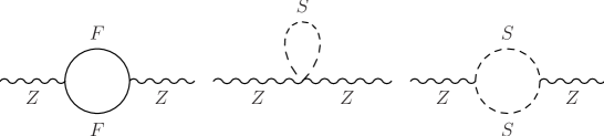
Figure 1: Generic one-loop Feynman-diagrams contributing to the neutral Higgs bosons renormalized self-energies (see text)

The analytical results for the unrenormalized self-energies and tadpoles are collected in the Appendix B. The final analytical results for the renormalized self-energies are easily obtained by inserting these results into (80).

We have checked that all the divergences involved in the computation cancel and the renormalized self-energies, $\hat{\Sigma}_{hh}(p^{2})$, $\hat{\Sigma}_{HH}(p^{2})$ and $\hat{\Sigma}_{hH}(p^{2})$ in the three schemes OS, $\overline{\mathrm{DR}}$, and m$\overline{\mathrm{DR}}$ are all finite, as expected. We have also checked that the renormalized self-energies in the OS scheme, are independent of the regularization scale $\mu_{\overline{\mathrm{DR}}}$, as they must be. The renormalized self-energies in the $\overline{\mathrm{DR}}$ are $\mu_{\overline{\mathrm{DR}}}$ dependent whereas the ones in the m$\overline{\mathrm{DR}}$ scheme are $\mu_{\overline{\mathrm{DR}}}$ independent by construction. Analytically they are related by $\hat{\Sigma}^{{\rm m}\overline{\mathrm{DR}}}(p^{2})=\hat{\Sigma}^{\overline{\mathrm{DR}}}(p^{2})|_{\mu_{\overline{\mathrm{DR}}}\,=\,m_{M}}$.

4.2 Analysis of the renormalized self-energies

In the following we discuss the numerical results for the renormalized self-energies. They are collected in Figs. 2 through 10. First we compare the predictions of the one-loop renormalized self-energies in the three schemes for the full interval $10^{3}\,\,{\rm GeV}\;\raisebox{-3.00003pt}{$\stackrel{{\scriptstyle\displaystyle<}}{{\sim}}$}\;m_{M}\;\raisebox{-3.00003pt}{$\stackrel{{\scriptstyle\displaystyle<}}{{\sim}}$}\;10^{15}\,\,{\rm GeV}$, and next we analyze these exact results at large $m_{M}$ with the help of the simple analytical formulas that are obtained in the seesaw limit. Then we choose the m$\overline{\mathrm{DR}}$ scheme and show the exact numerical results of the renormalized self-energies as functions of all the neutrino/sneutrino parameters involved. Finally we conclude on the subset of most relevant parameters (specifically, $m_{M}$, $m_{\tilde{R}}$, $B_{\nu}$ and $m_{\nu}$) which will be the selected ones to study the corrections to $M_{h}$ in the next subsection. For the final estimate of these corrections, and to localize the regions of the parameter space where they can reach sizeable values, we will vary these relevant parameters within some selected plausible intervals. For the parameters which do not exhibit a relevant numerical effect on $M_{h}$ (specifically, $\tan\beta$, $M_{A}$, $\mu$, $m_{\tilde{L}}$ and $A_{\nu}$) we choose representative values. For completeness, we will also comment shortly at the end of this subsection on the Dirac case.

In order to compare systematically our predictions of the neutrino/sneutrino sector in the MSSM-seesaw with those in the MSSM, we have split the full one-loop neutrino/sneutrino result into two parts:

$$\hat{\Sigma}(p^{2})|_{\rm full}=\hat{\Sigma}(p^{2})|_{\rm gauge}+\hat{\Sigma}(p^{2})|_{\rm Yukawa}~{},$$ (97)

where $\hat{\Sigma}(p^{2})|_{\rm gauge}$ means the contributions from pure gauge interactions and they are obtained by switching off the Yukawa interactions, i.e. by setting $Y_{\nu}=0$ (or equivalently $m_{D}=0$). The remaining part is named here $\hat{\Sigma}(p^{2})|_{\rm Yukawa}$ and refers to the contributions that are only present if $Y_{\nu}\neq 0$. In other words, this separation splits the full result into the common part with the MSSM, given by $\hat{\Sigma}(p^{2})|_{\rm gauge}$, and the new contributions due to the presence of Majorana neutrinos with non vanishing Yukawa interactions, given by $\hat{\Sigma}(p^{2})|_{\rm Yukawa}$. Thus, by comparing the size of these two parts, within the allowed parameter space region, we will localize the areas where $\hat{\Sigma}(p^{2})|_{\rm Yukawa}\gg\hat{\Sigma}(p^{2})|_{\rm gauge}$, which will therefore indicate a significant departure from the MSSM result.

Dependence on $m_{M}$

We show in Fig. 2 the predictions for $\hat{\Sigma}_{hh}(p^{2})$ as a function of $m_{M}$ in the three schemes: $\overline{\mathrm{DR}}$ (upper left plot), OS (upper right plot), and m$\overline{\mathrm{DR}}$ (lower left plot). In these plots we have considered an extremely wide range for the $m_{M}$ values, from $10^{3}\,\,\mathrm{GeV}$ up to $10^{15}\,\,\mathrm{GeV}$, and fixed the physical light neutrino mass to $|m_{\nu}|=0.5\,\,\mathrm{eV}$. Consequently, $m_{D}$ is derived from $m_{M}$ and $m_{\nu}$ by using (11) and (12). The other parameters are fixed as indicated in the figure. In this and in the following figures we have fixed $p^{2}$ in the self-energies to a particular value, corresponding to an approximation of the higher-order corrected value of $M_{h}$ for the input MSSM parameters set in each figure, see below. The numerical values used here and in the following for the SUSY parameters are representative values (as will also be shown below). Therefore, despite choosing only a few values for the parameters, the results obtained can be considered as more general.

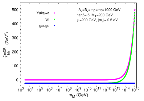
Figure 2: Renormalized Higgs boson self-energies as a function of $m_{M}$ and comparison between the three considered schemes. Upper left panel: $\hat{\Sigma}_{hh}^{\overline{\mathrm{DR}}}(p^{2})$. Upper right panel: $\hat{\Sigma}_{hh}^{\rm OS}(p^{2})$. Lower left panel: $\hat{\Sigma}_{hh}^{{\rm m}\overline{\mathrm{DR}}}(p^{2})$. Lower right panel: $\hat{\Sigma}_{hh}^{{\rm m}\overline{\mathrm{DR}}}(p^{2})$, $\hat{\Sigma}_{HH}^{{\rm m}\overline{\mathrm{DR}}}(p^{2})$ and $\hat{\Sigma}_{hH}^{{\rm m}\overline{\mathrm{DR}}}(p^{2})$. All self-energies are evaluated at $p^{2}=(116\,\,\mathrm{GeV})^{2}.$

In the three mentioned plots in Fig. 2 one can see that the numerical value of the full result is nearly constant with $m_{M}$ in the three schemes from $m_{M}=10^{3}\,\,\mathrm{GeV}$ up to $m_{M}\sim 10^{12}\,\,\mathrm{GeV}$. Furthermore, this constant value is approximately the same in the three schemes (the differences are below $\sim 10^{-2}$ ${\rm GeV}^{2}$), and is totally dominated by the ’pure gauge contributions’. Thus, for $10^{3}\,\,\mathrm{GeV}\;\raisebox{-3.00003pt}{$\stackrel{{\scriptstyle\displaystyle<}}{{\sim}}$}\;m_{M}\;\raisebox{-3.00003pt}{$\stackrel{{\scriptstyle\displaystyle<}}{{\sim}}$}\;10^{12}\,\,\mathrm{GeV}$ the result in the MSSM-seesaw nearly coincides with the result in the MSSM, irrespectively of the scheme. For the choice of input parameters in this plot, we get $\hat{\Sigma}_{hh}|_{\rm full}\simeq\hat{\Sigma}_{hh}|_{\rm gauge}\simeq-23.67\,\,\mathrm{GeV}^{2}$.

For larger values of $m_{M}$ in the range $10^{12}\,\,\mathrm{GeV}\,<\,m_{M}\,<\,10^{15}\,\,\mathrm{GeV}$, there are, however, remarkable differences between the three considered schemes, and the main differences come clearly from the ’Yukawa contributions’. Whereas $\hat{\Sigma}_{hh}^{\rm OS}|_{\rm full}$ is apparently constant with $m_{M}$, also for $m_{M}>10^{12}\,\,\mathrm{GeV}$, $|\hat{\Sigma}_{hh}^{\overline{\mathrm{DR}}}|_{\rm full}|$ and $|\hat{\Sigma}_{hh}^{m\overline{\mathrm{DR}}}|_{\rm full}|$ grow noticeably with $m_{M}$ at these large $m_{M}$ values. The numerical value of $\hat{\Sigma}_{hh}^{\overline{\mathrm{DR}}}|_{\rm full}$ is negative for $m_{M}>10^{12}\,\,\mathrm{GeV}$ and gets large values in this range, where they are totally dominated by the ’Yukawa contributions’. For instance, for $m_{M}=10^{13}\,\,\mathrm{GeV}$, we get $\hat{\Sigma}_{hh}^{\overline{\mathrm{DR}}}|_{\rm full}\simeq\hat{\Sigma}_{hh}^{\overline{\mathrm{DR}}}|_{\rm Yukawa}\simeq-250\,\,\mathrm{GeV}^{2}$, and for $m_{M}=10^{14}\,\,\mathrm{GeV}$, we get $\hat{\Sigma}_{hh}^{\overline{\mathrm{DR}}}|_{\rm full}\simeq\hat{\Sigma}_{hh}^{\overline{\mathrm{DR}}}|_{\rm Yukawa}\simeq-3000\,\,\mathrm{GeV}^{2}$. In the m$\overline{\mathrm{DR}}$ scheme, the result is negative up to $5\times 10^{13}\,\,\mathrm{GeV}$ and then becomes positive and large for $m_{M}>5\times 10^{13}\,\,\mathrm{GeV}$. Notice that, the absolute value in the m$\overline{\mathrm{DR}}$ scheme at large $m_{M}$ is always smaller than in the $\overline{\mathrm{DR}}$ scheme, due to the commented cancellation of the large logarithms $\log(m_{M}/\mu_{\overline{\mathrm{DR}}})$ corresponding to the choice $\mu_{\overline{\mathrm{DR}}}=m_{M}$. Notice also that, in spite of this cancellation, the size of the corrections in m$\overline{\mathrm{DR}}$, are still large for large enough $m_{M}$ values. For instance, for $m_{M}=10^{15}\,\,\mathrm{GeV}$, we get dominance of the ’Yukawa contributions’ $\hat{\Sigma}_{hh}^{m\overline{\mathrm{DR}}}|_{\rm full}\simeq\hat{\Sigma}_{hh}^{m\overline{\mathrm{DR}}}|_{\rm Yukawa}\simeq 500\,\,\mathrm{GeV}^{2}$. In contrast, for $m_{M}=10^{14}\,\,\mathrm{GeV}$, the ’Yukawa contributions’ and the ’pure gauge contributions’, compete since $\hat{\Sigma}_{hh}^{m\overline{\mathrm{DR}}}|_{\rm Yukawa}\simeq 60\,\,\mathrm{GeV}^{2}$ and $\hat{\Sigma}_{hh}^{m\overline{\mathrm{DR}}}|_{\rm gauge}\simeq-24\,\,\mathrm{GeV}^{2}$ leading to $\hat{\Sigma}_{hh}^{m\overline{\mathrm{DR}}}|_{\rm full}\simeq 36\,\,\mathrm{GeV}^{2}$.

In the lower right plot of Fig. 2 we compare $\hat{\Sigma}_{hh}^{m\overline{\mathrm{DR}}}|_{\rm full}$ to the other two renormalized self-energies, $\hat{\Sigma}_{HH}^{m\overline{\mathrm{DR}}}|_{\rm full}$ and $\hat{\Sigma}_{hH}^{m\overline{\mathrm{DR}}}|_{\rm full}$. One can observe that the three self-energies behave qualitatively very similarly with $m_{M}$, being approximately constant for $m_{M}<10^{12}\,\,\mathrm{GeV}$ and growing (in modulus) with $m_{M}$ for $10^{12}\,\,\mathrm{GeV}\,<\,m_{M}\,<\,10^{15}\,\,\mathrm{GeV}$. For the choice of parameters in this plot, $|\hat{\Sigma}_{hh}^{m\overline{\mathrm{DR}}}|_{\rm full}|$ is larger than the others in the full explored $m_{M}$ range. This will be relevant for the forthcoming estimate of the one-loop radiative corrections to $M_{h}$.

The previously commented growing behavior of the renormalized self-energies with $m_{M}$ is a consequence of the corresponding growing behavior of the neutrino Yukawa interactions with $m_{M}$, see (11) and (12). This is a well known feature of the seesaw models that, in order to get the light neutrino masses $m_{\nu}$ in agreement with data, one must impose for each input $m_{M}$ value the proper $Y_{\nu}$ (and therefore $m_{D}$) to precisely match the experimentally inspired input $m_{\nu}$. $Y_{\nu}$ is therefore not an input but an output in this approach, and according to (11) and (12) $Y_{\nu}$ grows with $m_{M}$ as $Y_{\nu}\propto\sqrt{m_{M}}$. The behavior of the renormalized self-energies with $m_{M}$ is, consequently, the result of the two competing facts, the increase of $Y_{\nu}$ with $m_{M}$ and the decreasing with $m_{M}$ from the neutrino and sneutrino propagators in the loops.

Dependence on $m_{M}$ in the seesaw limit

In order to illustrate more clearly the behavior with $m_{M}$, we have analyzed in more detail the renormalized self-energies in the seesaw limit, as defined in section 2. As the increase with $m_{M}$ starts at very large $m_{M}>10^{12}\,\,\mathrm{GeV}$ values (i.e. much larger than the other scales, $m_{M}\gg m_{D},M_{Z},M_{A},\mu,m_{\tilde{L}},m_{\tilde{R}},B_{\nu},A_{\nu}$), one expects that this limit should approximate pretty well the full result and show its same main features.

For the computation of the renormalized self-energies in this seesaw limit, we have performed a systematic expansion of the exact result in powers of the seesaw parameter $\xi=m_{D}/m_{M}$. In order to reduce the number of parameters, and for a clearer interpretation of the results, we have set in this expansion, $A_{\nu}=\mu=B_{\nu}=0$ (which is justified, see below) and we have assumed universal soft SUSY breaking masses, i.e., $m_{\tilde{L}}=m_{\tilde{R}}=m_{\rm SUSY}$.

The analytical expressions for these expanded renormalized self-energies are of the generic form:

$$\hat{\Sigma}(p^{2})=\left(\hat{\Sigma}(p^{2})\right)_{m_{D}^{0}}+\left(\hat{\Sigma}(p^{2})\right)_{m_{D}^{2}}+\left(\hat{\Sigma}(p^{2})\right)_{m_{D}^{4}}+\ldots~{},$$ (98)

where, $\left(\hat{\Sigma}(p^{2})\right)_{m_{D}^{0}}$ is the first term in the expansion, i.e. ${\cal O}(\xi^{0})$, $\left(\hat{\Sigma}(p^{2})\right)_{m_{D}^{2}}$ is the next term, i.e.${\cal O}(\xi^{2})$, $\left(\hat{\Sigma}(p^{2})\right)_{m_{D}^{4}}$ is the term of ${\cal O}(\xi^{4})$, etc. It should be noticed that there are no terms with odd powers of $\xi$. The first term in this expansion is precisely the pure gauge contribution, $\left(\hat{\Sigma}(p^{2})\right)_{m_{D}^{0}}=\hat{\Sigma}(p^{2})|_{\rm gauge}$. Therefore, it approximates the result in the MSSM and the rest approximates the Yukawa part,

$$\left(\hat{\Sigma}(p^{2})\right)_{\rm MSSM} \simeq\left(\hat{\Sigma}(p^{2})\right)_{m_{D}^{0}}~{},$$

$$\left(\hat{\Sigma}(p^{2})\right)_{\rm Yukawa} \simeq\left(\hat{\Sigma}(p^{2})\right)_{m_{D}^{2}}+\left(\hat{\Sigma}(p^{2})\right)_{m_{D}^{4}}+\ldots~{}.$$ (99)

In order to get simple formulas, we have expanded in addition each term in the series in (98) in powers of the other small dimensionless parameters, namely, $M_{Z}/m_{M}$, $M_{A}/m_{M}$, $p/m_{M}$ and $m_{\rm SUSY}/m_{M}$.

The result of the previous seesaw expansion (we just show the leading terms; terms suppressed by factors $1/m_{M}^{2}$ respect to these leading ones are not relevant and, therefore, are not included) for each of the three considered renormalization schemes is as follows.

${\cal O}(m_{D}^{0})$

$$\left(\hat{\Sigma}_{hh}^{\overline{\mathrm{DR}}}(p^{2})\right)_{m_{D}^{0}} =\frac{g^{2}M_{Z}^{2}\sin^{2}(\alpha+\beta)}{1152c_{\mathrm{w}}^{2}m_{\rm SUSY}^{2}\pi^{2}}\Big{[}-20m_{\rm SUSY}^{2}+3p^{2}+12m_{\rm SUSY}^{2}\log\frac{M_{Z}^{2}}{m_{\rm SUSY}^{2}}\Big{]}$$ (100a)

$$\left(\hat{\Sigma}_{hh}^{\mathrm{m}\overline{\mathrm{DR}}}(p^{2})\right)_{m_{D}^{0}} =\left(\hat{\Sigma}_{hh}^{\overline{\mathrm{DR}}}(p^{2})\right)_{m_{D}^{0}}$$ (100b)

$$\left(\hat{\Sigma}_{hh}^{\rm OS}(p^{2})\right)_{m_{D}^{0}} =\left(\hat{\Sigma}_{hh}^{\overline{\mathrm{DR}}}(p^{2})\right)_{m_{D}^{0}}+\frac{g^{2}M_{Z}^{2}}{3072c_{\mathrm{w}}^{2}m_{\rm SUSY}^{2}\pi^{2}}\Big{[}4\left(p^{2}-m_{h}^{2}\right)\left(\cos 2\alpha\cos 2\beta-1\right)$$

$$+\sec 2\alpha\sin 2\beta\left(M_{A}^{2}\left(\sin 4\beta-\sin 4\alpha\right)-M_{Z}^{2}\sin 4(\alpha+\beta)\right)\Big{]}$$ (100c)

${\cal O}(m_{D}^{2})$

$$\left(\hat{\Sigma}_{hh}^{\overline{\mathrm{DR}}}(p^{2})\right)_{m_{D}^{2}} =\frac{g^{2}m_{D}^{2}}{64\pi^{2}M_{W}^{2}\sin^{2}\beta}\left[1-\log\frac{m_{M}^{2}}{\mu_{\overline{\mathrm{DR}}}^{2}}\right]\left[-2M_{A}^{2}\cos^{2}(\alpha-\beta)\cos^{2}\beta\right.$$

$$\left.+2p^{2}\cos^{2}\alpha-M_{Z}^{2}\sin\beta\sin(\alpha+\beta)\left(2\left(1+\cos^{2}\beta\right)\cos\alpha-\sin 2\beta\sin\alpha\right)\right]$$ (101a)

$$\left(\hat{\Sigma}_{hh}^{\mathrm{m}\overline{\mathrm{DR}}}(p^{2})\right)_{m_{D}^{2}} =\left(\hat{\Sigma}_{hh}^{\overline{\mathrm{DR}}}(p^{2})\right)_{m_{D}^{2}\Big{|}\mu_{\overline{\mathrm{DR}}}=m_{M}}$$ (101b)

$$\left(\hat{\Sigma}_{hh}^{\rm OS}(p^{2})\right)_{m_{D}^{2}} =\frac{gm_{D}^{2}}{768\pi^{2}M_{W}^{2}p^{2}m_{M}^{2}}\Big{[}12m_{\rm SUSY}^{2}\Big{[}M_{A}^{2}p^{2}\left(2\cos^{2}(\alpha-\beta)\cot^{2}\beta-\cot\beta\sin 2(\alpha-\beta)\right)$$

$$-2m_{h}^{2}p^{2}\cos^{2}\alpha\csc^{2}\beta-4M_{Z}^{2}p^{2}\cos\alpha\csc\beta\sin(\alpha+\beta)+4M_{Z}^{4}\sin^{2}(\alpha+\beta)$$

$$+2M_{Z}^{2}p^{2}\sin^{2}(\alpha+\beta)-M_{Z}^{2}p^{2}\cot\beta\sin 2(\alpha+\beta)-4M_{Z}^{2}p^{2}\sin^{2}(\alpha+\beta)\log\frac{M_{Z}^{2}}{m_{M}^{2}}$$

$$+4M_{Z}^{4}\sin^{2}(\alpha+\beta)\log\frac{p^{2}}{m_{M}^{2}}-\log\frac{m_{\rm SUSY}^{2}}{m_{M}^{2}}\Big{[}2m_{h}^{2}p^{2}\cos^{2}\alpha\csc^{2}\beta+4M_{Z}^{4}\sin^{2}(\alpha+\beta)$$

$$-M_{Z}^{2}p^{2}\left(2\sin^{2}(\alpha+\beta)-\cot\beta\sin 2(\alpha+\beta)+4\cos\alpha\csc\beta\sin(\alpha+\beta)\right)$$

$$+M_{A}^{2}p^{2}\left(\cot\beta\sin 2(\alpha-\beta)-2\cot^{2}\beta\cos^{2}(\alpha-\beta)\right)\Big{]}\Big{]}$$

$$+p^{2}\Big{[}8M_{A}^{4}\cos^{2}(\alpha-\beta)\cot^{2}\beta+8\cos^{2}\alpha\left(3M_{Z}^{2}\left(m_{h}^{2}-p^{2}\right)+p^{2}\csc^{2}\beta\left(3m_{h}^{2}-p^{2}\right)\right)$$

$$+24M_{Z}^{2}p^{2}\cos\alpha\csc\beta\sin(\alpha+\beta)+12M_{A}^{2}M_{Z}^{2}\cos^{2}\beta\cos 2\beta\sec 2\alpha$$

$$+12M_{Z}^{4}\sin^{2}(\alpha+\beta)(-1+2\log\frac{M_{Z}^{2}}{p^{2}})+3\cot\beta\Big{[}-2M_{A}^{2}M_{Z}^{2}\sin 2\alpha$$

$$+2\sec 2\alpha\big{[}-M_{A}^{2}\sin 2(\alpha-\beta)\left(-M_{A}^{2}+2m_{h}^{2}-M_{Z}^{2}+M_{A}^{2}\cos 2\alpha\right)$$

$$+M_{Z}^{2}\sin 2(\alpha+\beta)\left(M_{A}^{2}-2m_{h}^{2}+M_{Z}^{2}-M_{A}^{2}\cos 2\alpha-M_{Z}^{2}\cos 2(\alpha+\beta)\right)\big{]}\Big{]}\Big{]}\Big{]}$$ (101c)

${\cal O}(m_{D}^{4})$

$$\left(\hat{\Sigma}_{hh}^{\overline{\mathrm{DR}}}(p^{2})\right)_{m_{D}^{4}} =\frac{g^{2}m_{D}^{4}}{128\pi^{2}M_{W}^{2}m_{M}^{2}p^{4}}\Big{[}4M_{Z}^{2}p^{2}\left(p^{2}-M_{Z}^{2}\right)\log\frac{m_{\rm SUSY}^{2}}{m_{M}^{2}}\sin^{2}(\alpha+\beta)$$

$$+8M_{A}^{2}p^{4}\cos^{2}(\alpha-\beta)\cot^{2}\beta\log\frac{M_{A}^{2}}{m_{M}^{2}}+4\left(2m_{\rm SUSY}^{2}-3M_{Z}^{2}\right)p^{4}\sin^{2}(\alpha+\beta)\log\frac{M_{Z}^{2}}{m_{M}^{2}}$$

$$+8p^{4}\csc^{2}\beta\big{[}M_{A}^{2}\cos^{2}\beta\cos^{2}(\alpha-\beta)-p^{2}\cos^{2}\alpha\big{]}$$

$$+8M_{Z}^{2}\sin(\alpha+\beta)p^{4}\big{[}2\cos\alpha\csc\beta-\sin(\alpha+\beta)\big{]}$$

$$+4m_{\rm SUSY}^{2}\log\frac{m_{\rm SUSY}^{2}}{m_{M}^{2}}\big{[}p^{4}\left(-1+\cos 2(\alpha+\beta)-4\cos^{2}\alpha\csc^{2}\beta\right)$$

$$+8M_{Z}^{2}p^{2}\cos\alpha\csc\beta\sin(\alpha+\beta)-2M_{Z}^{4}\sin^{2}(\alpha+\beta)\big{]}$$

$$-4\log\frac{p^{2}}{m_{M}^{2}}\big{[}2p^{6}\cos^{2}\alpha\csc^{2}\beta+4M_{Z}^{2}p^{2}\left(2m_{\rm SUSY}^{2}-p^{2}\right)\cos\alpha\csc\beta\sin(\alpha+\beta)$$

$$-M_{Z}^{4}\sin^{2}(\alpha+\beta)\left(2m_{\rm SUSY}^{2}+p^{2}\right)\big{]}-8m_{\rm SUSY}^{2}\big{[}2p^{4}\cos^{2}\alpha\csc^{2}\beta$$

$$+4M_{Z}^{2}p^{2}\cos\alpha\csc\beta\sin(\alpha+\beta)+\sin^{2}(\alpha+\beta)\left(M_{Z}^{4}-p^{4}\right)\big{]}\Big{]}$$ (102a)

$$\left(\hat{\Sigma}_{hh}^{{\rm m}\overline{\mathrm{DR}}}(p^{2})\right)_{m_{D}^{4}} =\left(\hat{\Sigma}_{hh}^{\overline{\mathrm{DR}}}(p^{2})\right)_{m_{D}^{4}}$$ (102b)

$$\left(\hat{\Sigma}_{hh}^{\rm OS}(p^{2})\right)_{m_{D}^{4}} =\left(\hat{\Sigma}_{hh}^{\overline{\mathrm{DR}}}(p^{2})\right)_{m_{D}^{4}}+\frac{g^{2}m_{D}^{4}}{32\pi^{2}M_{W}^{2}m_{M}^{2}}\Big{[}\cot\beta\sec 2\alpha\sin^{2}\alpha\big{[}M_{A}^{2}\sin 2(\alpha-\beta)$$

$$+M_{Z}^{2}\sin 2(\alpha+\beta)\big{]}\Big{[}2+\log\frac{m_{H}^{2}}{m_{M}^{2}}\Big{]}-\cos^{2}\alpha\Big{[}2+\log\frac{m_{h}^{2}}{m_{M}^{2}}\Big{]}\big{[}2(m_{h}^{2}-p^{2})\csc^{2}\beta$$

$$+\cot\beta\sec 2\alpha\big{[}M_{A}^{2}\sin 2(\alpha-\beta)+M_{Z}^{2}\sin 2(\alpha+\beta)\big{]}\big{]}\Big{]}$$ (102c)

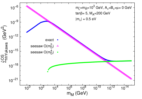
Figure 3: Comparison between the predictions from the seesaw expansion and the exact results for the Yukawa part. Left panel: m$\overline{\mathrm{DR}}$ scheme. Right panel: OS scheme. In both panels, $p^{2}=(116\,\,\mathrm{GeV})^{2}$.

From these formulas the qualitatively different behavior of the renormalized Higgs-boson self-energies on the Majorana mass scale $m_{M}$ can be understood. The main difference between the OS scheme and the $\overline{\mathrm{DR}}$/$\mathrm{m}\overline{\mathrm{DR}}$ schemes appears in the Yukawa part, especially in the term of ${\cal O}(m_{D}^{2})$. At the various orders the comparison of the three schemes is given as follows.

At the leading order in the seesaw expansion, ${\cal O}(m_{D}^{0})$ in (100), the results in the $\overline{\mathrm{DR}}$ and m$\overline{\mathrm{DR}}$ schemes coincide. This is indeed a consequence of the fact that, at this order, $\hat{\Sigma}_{hh}^{\overline{\mathrm{DR}}}(p^{2})$ turns out to be $\mu_{\overline{\mathrm{DR}}}$ independent. The result in the OS scheme differs from these later by a term of order $g^{2}M_{Z}^{2}M_{\rm EW}^{2}/m_{\rm SUSY}^{2}$, where $M_{\rm EW}^{2}$ refers generically to the involved masses of the order of the electroweak scale, i.e., $M_{A}^{2}$, $p^{2}$, $M_{Z}^{2}$, $m_{h\,{\rm tree}}^{2}$. Furthermore, this difference turns out to be numerically extremely small. This explains why, for low values of the Majorana scale, where the ${\cal O}(m_{D}^{0})$ term of the expansion dominates, the predictions from the three schemes are nearly indistinguishable.

At the next order in the seesaw expansion, ${\cal O}(m_{D}^{2})$ in (101), the OS result differs substantially from the $\overline{\mathrm{DR}}$ and $\mathrm{m}\overline{\mathrm{DR}}$ schemes. First, the OS result is extremely suppressed with respect to the $\overline{\mathrm{DR}}$ and $\mathrm{m}\overline{\mathrm{DR}}$ results at large $m_{M}$. This is due to the fact that the leading contribution, i.e. of the order of $g^{2}m_{D}^{2}M_{\rm EW}^{2}/M_{Z}^{2}$, vanishes in the OS whereas it is present in the other schemes. As can be seen in (101), the first non vanishing contribution contains an extra factor $\sim m_{\rm SUSY}^{2}/m_{M}^{2}$ which can be extremely small for $m_{M}\gg m_{\rm SUSY}$. This remarkable difference of the OS result has its origin in the different values of the $\delta Z_{hh}$ and $\delta\tan\beta$ counterterms. More specifically, by computing their finite parts in the OS scheme and in the seesaw limit, we get

$$\delta^{\rm OS}Z_{hh}|_{\rm finite} =-\frac{g^{2}m_{D}^{2}\cos^{2}\!\alpha\,}{32c_{\mathrm{w}}^{2}M_{Z}^{2}\pi^{2}\sin^{2}\beta}\left[1-\log\frac{m_{M}^{2}}{\mu_{\overline{\mathrm{DR}}}^{2}}\right]+{\cal O}\left(\frac{M_{\rm EW}^{2},m_{\rm SUSY}^{2}}{m_{M}^{2}}\right),$$ (103)

$$\delta^{\rm OS}\tan\beta|_{\rm finite} =-\frac{g^{2}m_{D}^{2}}{64c_{\mathrm{w}}^{2}M_{Z}^{2}\pi^{2}\sin^{2}\beta}\left[1-\log\frac{m_{M}^{2}}{\mu_{\overline{\mathrm{DR}}}^{2}}\right]+{\cal O}\left(\frac{M_{\rm EW}^{2},m_{\rm SUSY}^{2}}{m_{M}^{2}}\right)~{}.$$ (104)

These finite contributions lead to the cancellation of the above commented leading contributions.

In the $\overline{\mathrm{DR}}$ scheme, we get an explicit logarithmic dependence on $m_{M}$, concretely as $-\log(m_{M}^{2}/\mu_{\overline{\mathrm{DR}}}^{2})$. By construction this term is absent in the $\mathrm{m}\overline{\mathrm{DR}}$ result. Therefore, the main difference between these two schemes $\overline{\mathrm{DR}}$ and $\mathrm{m}\overline{\mathrm{DR}}$ is this logarithmic contribution that can be sizeable for very large $m_{M}\gg\mu_{\overline{\mathrm{DR}}}$.

The results at the next to next order in the seesaw expansion, ${\cal O}(m_{D}^{4})$ in (102), show that they all go (leaving apart the logarithms) as $g^{2}m_{D}^{4}(M_{\rm EW}^{2},m_{\rm SUSY}^{2})/(M_{Z}^{2}m_{M}^{2})$. Therefore the ${\cal O}(m_{D}^{4})$ terms are extremely suppressed in the three schemes, and consequently they are not relevant in the large $m_{M}$ regime.

All the above commented analytical features of the seesaw expansion have also been checked numerically, as it is illustrated in Fig. 3. In this figure we show separately the ${\cal O}(m_{D}^{2})$ and ${\cal O}(m_{D}^{4})$ contributions and the exact Yukawa prediction in both the $\mathrm{m}\overline{\mathrm{DR}}$ (left plot) and OS scheme (right plot). One clearly observes the dominance of the ${\cal O}(m_{D}^{2})$ over the ${\cal O}(m_{D}^{4})$ in the $\mathrm{m}\overline{\mathrm{DR}}$ scheme by many orders of magnitude in the full explored $m_{M}$ range. One also sees that the ${\cal O}(m_{D}^{2})$ result approximates extremely well the exact Yukawa result for $m_{M}\;\raisebox{-3.00003pt}{$\stackrel{{\scriptstyle\displaystyle>}}{{\sim}}$}\;10^{4}\,\,\mathrm{GeV}$. In contrast, in the OS scheme, the ${\cal O}(m_{D}^{2})$ term dominates just up to about $m_{M}=10^{10}\,\,\mathrm{GeV}$, but then for larger values the ${\cal O}(m_{D}^{4})$ dominates. In this plot it is also manifested that the exact Yukawa result in the OS is well approximated by the ${\cal O}(m_{D}^{2})$ term in the interval $10^{3}\,\,\mathrm{GeV}<m_{M}<10^{11}\,\,\mathrm{GeV}$ and by the ${\cal O}(m_{D}^{4})$ term for $m_{M}>10^{12}\,\,\mathrm{GeV}$. At this large values, however, the size of the correction is extremely small (below $10^{-17}$ ${\rm GeV}^{2}$), hence, irrelevant. It is also clear from this plot that the numerical results for the ${\cal O}(m_{D}^{4})$ contributions are similar in the three schemes.

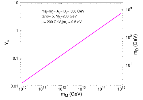
Figure 4: Left panel: Decoupling/Non-decoupling behavior of the one-loop neutrino/sneutrino corrections to the renormalized lightest Higgs boson self-energy at large $m_{M}$ in the $\mathrm{m}\overline{\mathrm{DR}}$ scheme. Right panel: Dependence of the neutrino Yukawa coupling (and $m_{D}$) with $m_{M}$.

From the definition of the three renormalization schemes, see Sect. 3.2, and our analytical and numerical analysis in this section we conclude that the $\mathrm{m}\overline{\mathrm{DR}}$ scheme is best suited for higher-order calculations in MSSM-seesaw model. The other two schemes can lead to unphysically large corrections at the one-loop level. We will focus in the following on this scheme, and the numerical evaluation of $M_{h}^{\nu/\tilde{\nu}}$, see Sect. 4.3, will be performed solely in this “preferred” scheme.

Finally, in this context, we discuss the decoupling or non-decoupling behavior of the neutrino/sneutrino one-loop radiative corrections with the Majorana scale. According to Figs. 2 and 3, the Yukawa part of the renormalized self-energy in the $\mathrm{m}\overline{\mathrm{DR}}$ scheme grows with $m_{M}$. However, this does not constitute by itself a proof of non-decoupling of $m_{M}$ in the radiative corrections to $\hat{\Sigma}_{hh}^{\mathrm{m}\overline{\mathrm{DR}}}$ for asymptotically large $m_{M}$. To analyze this question, we have to investigate separately the behaviors of $\hat{\Sigma}_{hh}^{\mathrm{m}\overline{\mathrm{DR}}}$ and $m_{D}$ with $m_{M}$, since in the way the seesaw mechanism is implemented here, as we have mentioned before, $m_{D}$ (or equivalently $Y_{\nu}$) is not an input but an output and it grows proportional to $\sqrt{m_{M}}$. To analyze these two behaviors separately we show in the left plot of Fig. 4 the ratio $(\hat{\Sigma}_{hh}^{\mathrm{m}\overline{\mathrm{DR}}})_{\rm Yukawa}/m_{D}^{2}$ versus $m_{M}$ (and $m_{D}$), and in the right plot we show the predictions of the Yukawa coupling (and $m_{D}$) as a function of $m_{M}$. The latter one exhibits the (trivial) result of $Y_{\nu}\propto\sqrt{m_{M}}$ as expected. In the left plot a constant behavior of the ratio $(\hat{\Sigma}_{hh}^{\mathrm{m}\overline{\mathrm{DR}}})_{\rm Yukawa}/m_{D}^{2}$ is clearly manifested, which means that the growing of $(\hat{\Sigma}_{hh}^{\mathrm{m}\overline{\mathrm{DR}}})_{\rm Yukawa}$ with $m_{M}$ is exclusively due to the growing of $Y_{\nu}$ (or $m_{D}$) with $m_{M}$. However, still this ratio turns out to be non-vanishing for asymptotically large $m_{M}$, and constant with $m_{D}$, as can be seen in Fig. 4. Therefore, a non-decoupling constant behavior must be concluded in the Majorana case from all this discussion. This constant, on the other hand, is very well approximated by the coefficient multiplying the factor $m_{D}^{2}$ in the $\hat{\Sigma}_{hh}^{\mathrm{m}\overline{\mathrm{DR}}}(p^{2})_{m_{D}^{2}}$ result of (101).

In order to understand this issue better, we compare this analytical result, showing a constant behaviour of the renormalized Higgs boson self-energy in the $m_{M}\to\infty$ limit when $Y_{\nu}$ is kept fixed, with the corresponding result in the Dirac case. For simplification in this analytical comparison we focus just on the ${\cal O}(p^{2}m_{D}^{2})$ terms and use the electroweak basis for neutrinos and sneutrinos. The results at ${\cal O}(p^{2}m_{D}^{2})$ for the renormalized self-energies in the $\overline{\mathrm{DR}}$ scheme for the Majorana and Dirac cases are:

$$\hat{\Sigma}_{hh}^{{\rm Majorana},\overline{\mathrm{DR}}}(p^{2}) = \frac{g^{2}m_{D}^{2}p^{2}\cos^{2}\alpha}{32\pi^{2}M_{W}^{2}\sin^{2}\beta}(\frac{1}{2}-\log\frac{m_{M}^{2}}{\mu_{\overline{\mathrm{DR}}}^{2}})$$ (105)

$$+\frac{g^{2}m_{D}^{2}p^{2}\cos^{2}\alpha}{64\pi^{2}M_{W}^{2}\sin^{2}\beta}$$

$$\hat{\Sigma}_{hh}^{{\rm Dirac},\overline{\mathrm{DR}}}(p^{2}) = \frac{g^{2}m_{D}^{2}p^{2}\cos^{2}\alpha}{32\pi^{2}M_{W}^{2}\sin^{2}\beta}(2-\log\frac{p^{2}}{\mu_{\overline{\mathrm{DR}}}^{2}})$$ (106)

where the first and second lines in $\hat{\Sigma}_{hh}^{{\rm Majorana},\overline{\mathrm{DR}}}(p^{2})$ are the contributions from neutrinos and sneutrinos respectively. It should be noticed that the ${\cal O}(p^{2}m_{D}^{2})$ sneutrino contributions come exclusively from the new couplings $g^{\prime}_{h\tilde{\nu}_{L}\tilde{\nu}_{R}}=-\frac{igm_{D}m_{M}\cos\alpha}{2M_{W}\sin\beta}$, which are not present in the Dirac case. It should also be noticed that this result in the Majorana case translates into our ${\cal O}(p^{2}m_{D}^{2})$ term in (101a). The comparison of the two formulas shows that the result of the Majorana case for low momenta, $p^{2}\ll m_{M}^{2}$, does not coincide with the result of the Dirac case.

From the right plot in Fig. 4 we can also conclude on the range of $m_{M}$ values where the neutrino Yukawa couplings get too large and potentialy non-perturbative. The concrete crossing line to set the perturbativity region is not uniquely defined, but it should be considered around $Y_{\nu}\sim{\cal O}(1)$. For instance, by setting the crossing at $Y_{\nu}^{2}/(4\pi)=1.5$ ($Y_{\nu}=4.34$) we get perturbativity for $m_{M}<10^{15}\,\,\mathrm{GeV}$, and by setting it at $Y_{\nu}=1.5$ it is got for $m_{M}<10^{14}\,\,\mathrm{GeV}$. In the following of this subsection we set $m_{M}=10^{14}\,\,\mathrm{GeV}$ as our reference value.

Dependence on $\tan\beta$, $M_{A}$, $\mu$, $m_{\tilde{L}}$, $m_{\tilde{R}}$, $A_{\nu}$, $m_{\nu}$, $B_{\nu}$ and $p$

The behavior of the renormalized self-energy in the m$\overline{\mathrm{DR}}$ scheme with the other parameters entering in this computation are shown in Figs. 5 - 10. In all these plots we have included separately the gauge, Yukawa and total results for comparison.

First, the behavior with $\tan\beta$ is analyzed in the left plot of Fig. 5. It exhibits basically the expected features that can be inferred from the loop corrections of an up-type fermion/sfermion. The neutrino/sneutrino one-loop radiative corrections reach their maximum value at the lowest considered value of $\tan\beta$, $\tan\beta=2$ in this plot. For $\tan\beta>5$ the dependence is nearly flat. There are no relevant differences between the behaviors with $\tan\beta$ of the Yukawa and the gauge parts. From now on, we will set $\tan\beta=5$ as our reference value.

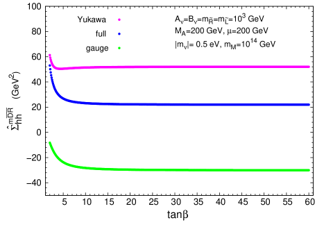
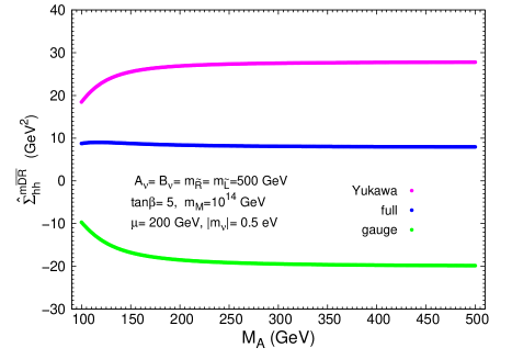
Figure 5: Left panel: $\hat{\Sigma}_{hh}^{\mathrm{m}\overline{\mathrm{DR}}}(p^{2})$ as a function of $\tan\beta$. Right panel: $\hat{\Sigma}_{hh}^{\mathrm{m}\overline{\mathrm{DR}}}(p^{2})$ as a function of $M_{A}$. In the left (right) panel, $p^{2}=(116\,\,{\rm GeV})^{2}$ ($p^{2}=(105\,\,\mathrm{GeV})^{2})$.

The behavior with $M_{A}$ is displayed in the right panel of Fig.5. Again we see no relevant differences with respect to the well known behavior in the MSSM. For $M_{A}$ larger that 150 GeV the total contribution from the neutrino/sneutrino sector to the renormalized self-energy is nearly flat with $M_{A}$. In the following we will take $M_{A}=200\,\,\mathrm{GeV}$ as our reference value.

The dependence with the soft SUSY breaking mass of the ‘left handed’ $SU(2)$ doublet, $m_{\tilde{L}}$, is shown in Fig. 6. We see that the gauge contribution is negative and increases in modulus with increasing $m_{\tilde{L}}$, whereas the Yukawa contribution is positive and nearly insensitive to changes of $m_{\tilde{L}}$ in the investigated interval, $10^{2}\,\,\mathrm{GeV}<m_{\tilde{L}}<10^{4}\,\,\mathrm{GeV}$. The total neutrino/sneutrino corrections, at these selected values of the model parameters, are positive and decreasing with $m_{\tilde{L}}$ for $10^{2}\,\,\mathrm{GeV}<m_{\tilde{L}}<2\times 10^{3}\,\,\mathrm{GeV}$ and then become negative and increasing in modulus with $m_{\tilde{L}}$ for $2\times 10^{3}\,\,\mathrm{GeV}<m_{\tilde{L}}<10^{4}\,\,\mathrm{GeV}$.

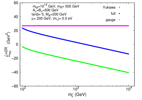
Figure 6: $\hat{\Sigma}_{hh}^{\mathrm{m}\overline{\mathrm{DR}}}(p^{2})$ as a function of $m_{\tilde{L}}$; we have set $p^{2}=(105\,\,\mathrm{GeV})^{2}$.

The behavior with the soft SUSY breaking parameter of the ‘right handed’ sector $m_{\tilde{R}}$ is shown in Fig. 7. In the left plot a mass scale similar to the other soft SUSY-breaking parameters is investigated, whereas in the right plot values of $m_{\tilde{R}}$ closer to $m_{M}$ are explored. It should be reminded that these values are not constrained by data. An interesting feature can be observed at large values of $m_{\tilde{R}}$. The contributions to the renormalized self-energy stay flat up to about $m_{\tilde{R}}\sim 10^{13}\,\,\mathrm{GeV}$. Above this mass scale the Yukawa part grows rapidly, reaching very large values at $m_{\tilde{R}}\sim 10^{14}\,\,\mathrm{GeV}$ of around $\hat{\Sigma}_{hh}^{\mathrm{m}\overline{\mathrm{DR}}}\sim 7000\,\,\mathrm{GeV}^{2}$.

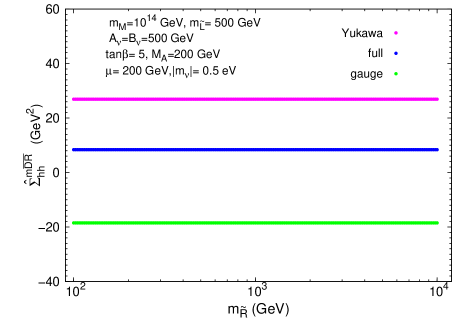
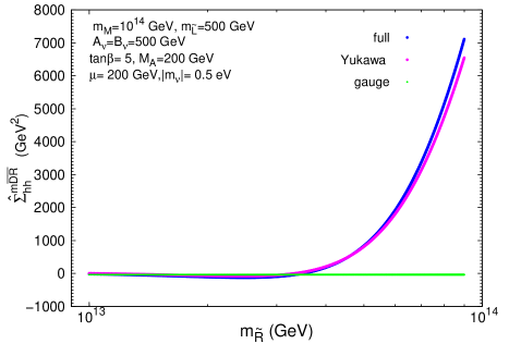
Figure 7: $\hat{\Sigma}_{hh}^{\mathrm{m}\overline{\mathrm{DR}}}(p^{2})$ as a function of $m_{\tilde{R}}$. Left panel: low mass values $10^{2}\,\,\mathrm{GeV}<m_{\tilde{R}}<10^{4}\,\,\mathrm{GeV}$. Right panel: high mass values $10^{13}\,\,\mathrm{GeV}<m_{\tilde{R}}<10^{14}\,\,\mathrm{GeV}$. In both panels we have set $p^{2}=(105\,\,\mathrm{GeV})^{2}$.

The behavior with the new soft SUSY-breaking trilinear coupling $A_{\nu}$ is shown in the left plot of Fig. 8. The full result, the gauge, and Yukawa parts are nearly independent on this parameter in the studied interval, $-1000\,\,\mathrm{GeV}<A_{\nu}<1000\,\,\mathrm{GeV}$. Although not shown explicitly, we have also studied the behavior with $\mu$ and got the same ‘flat’ behavior for $-1000\,\,\mathrm{GeV}<\mu<1000\,\,\mathrm{GeV}$. This justifies our choice $A_{\nu}=\mu=0$ in our seesaw expansion above.

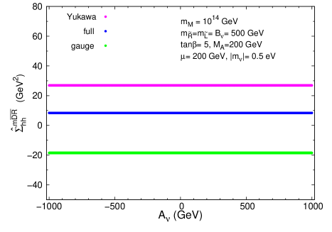
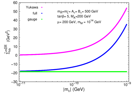
Figure 8: Left panel: $\hat{\Sigma}_{hh}^{\mathrm{m}\overline{\mathrm{DR}}}(p^{2})$ as a function of $A_{\nu}$. Right panel: $\hat{\Sigma}_{hh}^{\mathrm{m}\overline{\mathrm{DR}}}(p^{2})$ as a function of $|m_{\nu}|$. In both panels we have set $p^{2}=(105\,\,\mathrm{GeV})^{2}$.

The behavior with the lightest neutrino mass, $m_{\nu}$, is demonstrated in the right plot of Fig. 8. One can see that the Yukawa part is quite sensitive to this mass that we have varied in a plausible and compatible with data range. The growing of the result with $|m_{\nu}|$, for fixed $m_{M}$, is the consequence of the growing of $Y_{\nu}$ (or $m_{D}$) with $|m_{\nu}|$ since in this model they are correlated, as shown in (11) and (12).

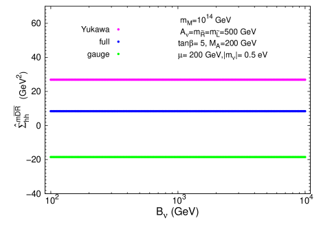
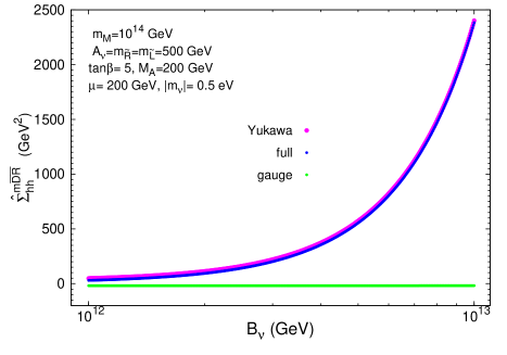
Figure 9: $\hat{\Sigma}_{hh}^{\mathrm{m}\overline{\mathrm{DR}}}(p^{2})$ as a function of $B_{\nu}$. Left panel: low $B_{\nu}$ values, $10^{2}\,\,\mathrm{GeV}<B_{\nu}<10^{4}\,\,\mathrm{GeV}$. Right panel: high $B_{\nu}$ values, $10^{12}\,\,\mathrm{GeV}<B_{\nu}<10^{13}\,\,\mathrm{GeV}$. In both panels we have set $p^{2}=(105\,\,\mathrm{GeV})^{2}$.

The behavior with $B_{\nu}$ is analyzed in Fig. 9. We have found a flat result with this new soft parameter for most of the explored range, except at very large values, $B_{\nu}>10^{12}\,\,\mathrm{GeV}$, as shown in the right plot. For these large values the Yukawa part grows noticeably with $B_{\nu}$ and dominates largely the total result, leading to large radiative corrections. For instance, for the parameters chosen in this figure and $B_{\nu}=10^{13}\,\,\mathrm{GeV}$, we found $\hat{\Sigma}_{hh}^{\mathrm{m}\overline{\mathrm{DR}}}\sim 2400\,\,\mathrm{GeV}^{2}$. The question whether such large values of $B_{\nu}$ are realistic depends on the particular models and universality conditions. However, such an analysis is beyond the scope of our paper. On the other hand, if we apply the bounds that are imposed in order to avoid destabilizing the electroweak symmetry breaking [13], leading to $B_{\nu}Y_{\nu}^{2}/(8\pi^{2})<m_{\rm SUSY}/\tan\beta$, one gets an upper limit on $B_{\nu}$. For $Y_{\nu}\sim 1$, $m_{\rm SUSY}\sim 1000\,\,\mathrm{GeV}$ and $\tan\beta\sim 5$ one finds $B_{\nu}<1.6\times 10^{4}\,\,\mathrm{GeV}$. For this range the renormalized Higgs-boson self-energy is nearly independent of $B_{\nu}$. From now on, we will choose $B_{\nu}=500\,\,\mathrm{GeV}$ as our reference value.

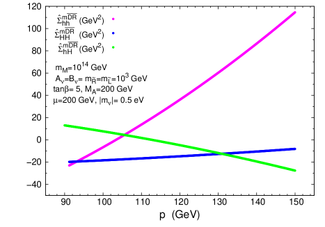
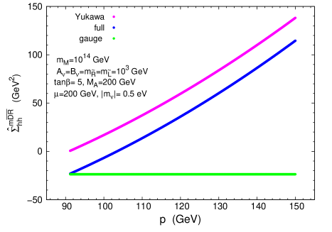
Figure 10: Left panel: $\hat{\Sigma}_{hh}^{\mathrm{m}\overline{\mathrm{DR}}}(p^{2})$, $\hat{\Sigma}_{hh}^{\mathrm{m}\overline{\mathrm{DR}}}(p^{2})$ and $\hat{\Sigma}_{hh}^{\mathrm{m}\overline{\mathrm{DR}}}(p^{2})$ as a function of the external momentum $p$. Right panel: the two contributions $\hat{\Sigma}_{hh}^{\mathrm{m}\overline{\mathrm{DR}}}(p^{2})_{\rm gauge}$ $\hat{\Sigma}_{hh}^{\mathrm{m}\overline{\mathrm{DR}}}(p^{2})_{\rm Yukawa}$ and the full result are shown separately.

Finally, we show in Fig. 10 the behavior with $p^{2}$, the square of the external momentum of the Higgs boson self-energies, which is a relevant issue for the discussion of the radiative corrections to the Higgs-boson masses (see the next subsection). The three renormalized self-energies, $\hat{\Sigma}_{hh}$, $\hat{\Sigma}_{HH}$ and $\hat{\Sigma}_{hH}$, are clearly dependent on $p^{2}$, but the most sensitive one is $\hat{\Sigma}_{hh}$. It is clear from this figure that setting $p^{2}=0$ in the renormalized self-energies does not provide a good approximation for the estimate of the radiative corrections to the Higgs boson mass from the neutrino/sneutrino sector in the present case of Majorana neutrinos. One can also see that mainly the Yukawa part is responsible for this sensitivity to $p^{2}$. Setting the proper $p^{2}$ in order to estimate realistically the Higgs mass corrections will be discussed in the next subsection.

The Dirac case

Finally, we perform a comparison between the case of massive Majorana neutrinos (as analyzed so far) and the case of Dirac neutrinos. In order to analyze the Dirac case, we have computed the one-loop neutrino/sneutrino contributions to the renormalized lightest Higgs boson self-energy for $m_{M}=0$. The analytical results for this Dirac case are collected in Appendix C. We have chosen here the $\overline{\mathrm{DR}}$ scheme, since due to the absence of $m_{M}$ no large logarithmic corrections are expected, and a comparison to existing calculations can readily be performed.

Figure 11: One-loop corrections to the Yukawa part of the lightest Higgs boson renormalized self-energy from the neutrino/sneutrino sector in the case of massive Dirac neutrinos

First, we have checked the finiteness of the result. Second, we have also checked that the obtained formulas agree with the well known result of the one-loop radiative corrections from other massive fermion/sfermion sectors of the MSSM, with the obvious corresponding changes of fermion/sfermion parameters and quantum numbers. In particular, it can be seen that the formulas in Appendix C coincide with the one-loop corrections from the MSSM top/stop sector by replacing, correspondingly, the neutrino $SU(2)\times U(1)$ quantum numbers by the top quark ones, $m_{D}$ by $m_{t}$, $m_{{\tilde{\nu}_{\pm}}}$ $(=m_{{\tilde{\nu}}_{1}})$ by $m_{{\tilde{t}}_{1}}$, $m_{{\tilde{N}_{\pm}}}$ $(=m_{{\tilde{\nu}}_{2}})$ by $m_{{\tilde{t}}_{2}}$, $\theta_{\pm}$ $(={\tilde{\theta}})$ by ${\tilde{\theta_{t}}}$ and by adding the proper color factor, $N_{C}=3$.

As for the numerical estimate, we present in Fig.11 the result of the Yukawa contributions from the one-loop neutrino/sneutrino radiative corrections to the renormalized self-energy, $(\hat{\Sigma}_{hh}^{\rm Yukawa})_{\rm Dirac}$, as a function of the physical neutrino mass, $|m_{\nu}|=m_{D}$. The regularization scale has been fixed here to $\mu_{\overline{\mathrm{DR}}}=100\,\,\mathrm{GeV}$ and the external momentum to $p=116\,\,\mathrm{GeV}$. As in the Majorana case, we consider an interval for the neutrino mass inspired by experimental data, $0.01\,\,{\rm eV}\;\raisebox{-3.00003pt}{$\stackrel{{\scriptstyle\displaystyle<}}{{\sim}}$}\;|m_{\nu}|\;\raisebox{-3.00003pt}{$\stackrel{{\scriptstyle\displaystyle<}}{{\sim}}$}\;1\,\,{\rm eV}$. In this plot we see clearly that, as expected, these Yukawa contributions are extremely small (below $10^{-20}$ ${\rm GeV}^{2}$) and are fully dominated by the gauge part which we have also estimated, for the chosen parameters in this plot, leading to $(\hat{\Sigma}_{hh}^{\rm gauge})_{\rm Dirac}=-18.5\,{\rm GeV^{2}}$. Notice that this gauge part is similar in both Majorana and Dirac cases, as can be seen in the right plot of Fig.8. In summary, the radiative corrections from the massive neutrinos/sneutrinos in the Dirac case are phenomenologically irrelevant and therefore this case is totally indistinguishable from the MSSM with massless neutrinos.

4.3 Estimate of the one-loop corrections from neutrino/sneutrino sector to $M_{h}$ within the MSSM-seesaw

We recall that the anticipated LHC precision of the mass of an SM-like Higgs boson is $\sim 200\,\,\mathrm{MeV}$, and that at the ILC an accuracy on the mass could reach the $50\,\,\mathrm{MeV}$ level. These experimental precisions set the goal for the theoretical accuracies.

As outlined in Sect. 3.1 the higher-order corrected light MSSM Higgs-boson mass is obtained as a pole from (75), i.e. where $p^{2}=M_{h}^{2}$. A realistic evaluation requires to take into account all known higher-order corrections to the renormalized Higgs-boson self-energies [42]. In order to simplify our analysis, but to maintain the high accuracy we follow a slightly different strategy. For a given set of SUSY parameters we first calculate $M_{h}$ and $M_{H}$ in the MSSM with the help of FeynHiggs [43, 44, 16, 33]. In this way all relevant known higher-order corrections are included, but no $\nu/\tilde{\nu}$ contributions are taken into account yet. This corresponds to a ‘diagonalization’ of the ${\cal CP}$-even Higgs sector in the MSSM without heavy Majorana (s)neutrinos. In a second step we search for the poles of

$$\left[p^{2}-M_{h}^{2}+\hat{\Sigma}_{hh}^{\nu/\tilde{\nu}}(M_{h}^{2})\right]\left[p^{2}-M_{H}^{2}+\hat{\Sigma}_{HH}^{\nu/\tilde{\nu}}(M_{h}^{2})\right]-\left[\hat{\Sigma}_{hH}^{\nu/\tilde{\nu}}(M_{h}^{2})\right]^{2}=0~{},$$ (107)

where, $\hat{\Sigma}_{hh,HH,hH}^{\nu/\tilde{\nu}}$ denote the full corrections to the renormalized Higgs-boson self-energies from the $\nu/\tilde{\nu}$ sector, obtained in the $\mathrm{m}\overline{\mathrm{DR}}$ scheme as described in the present work. The pole, the light Higgs mass including the $\nu/\tilde{\nu}$ corrections (i.e. in the MSSM-seesaw model), is denoted by $M_{h}^{\nu/\tilde{\nu}}$. This ‘re-diagonalization’ now effectively takes into account the full result of the MSSM-seesaw. The momentum in the self-energies is fixed to the value $M_{h}$ as obtained with FeynHiggs, since it is expected that the new contributions only give a relatively small correction to this $M_{h}$. In a more elaborate analysis the renormalized self-energies should be evaluated with free $p^{2}$. However, we expect only a very minor effect from fixing the external momentum to this value. In the near future the results of the new neutrino/sneutrino corrections will be implemented into the code FeynHiggs.

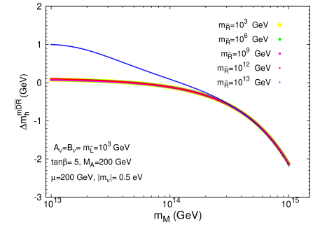
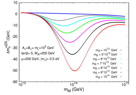
Figure 12: One-loop corrections to the lightest Higgs boson mass from the neutrino/sneutrino sector as a function of the heavy Majorana mass for various choices of the soft mass ${m_{\tilde{R}}}$. Left panel: ${m_{\tilde{R}}}<10^{13}\,\,\mathrm{GeV}$. Right panel:$10^{13}\,\,{\rm GeV}<{m_{\tilde{R}}}<10^{14}\,\,{\rm GeV}$.

The numerical results for $\Delta m_{h}^{\mathrm{m}\overline{\mathrm{DR}}}:=M_{h}^{\nu/\tilde{\nu}}-M_{h}$ are summarized in Figs. 12 through 15. We have chosen here to explore the Higgs mass predictions as a function of just the most relevant model parameters which, according to our previous exhaustive analysis of the renormalized Higgs-boson self-energies, are going to provide the most interesting/sizeable corrections. These are: the Majorana mass $m_{M}$ (or, equivalently, the heaviest physical Majorana neutrino mass $m_{N}$), the soft SUSY breaking parameters $m_{\tilde{R}}$ and $B_{\nu}$ and the lightest physical Majorana neutrino mass $m_{\nu}$. As for the numerical values of these relevant parameters, we focus here in the following intervals: $10^{13}\,\,{\rm GeV}\leq m_{M}\leq 10^{15}\,\,{\rm GeV}$, $0.1\,\,{\rm eV}\leq|m_{\nu}|\leq 1\,\,{\rm eV}$, $10^{3}\,\,{\rm GeV}\leq m_{\tilde{R}}\leq m_{M}$ and $10^{3}\,\,{\rm GeV}\leq B_{\nu}\leq 4\times 10^{12}\,\,{\rm GeV}$. For the remaining model parameters, $\tan\beta$, $M_{A}$, $\mu$, $m_{\tilde{L}}$ and $A_{\nu}$, we choose here the same reference values as in the previous subsection. The corresponding predictions for other choices of the parameters can be easily inferred from our previous results of the renormalized self-energies.

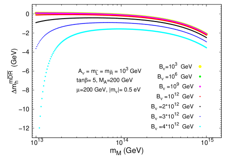
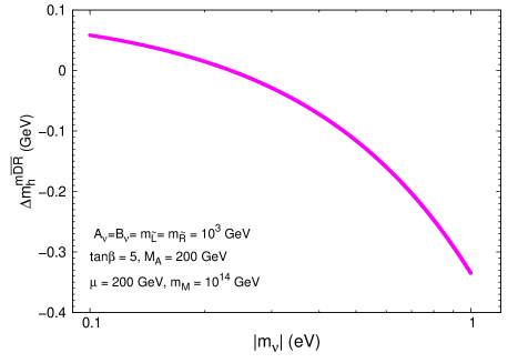
Figure 13: Left panel: One-loop corrections to the lightest Higgs boson mass from the neutrino/sneutrino sector as a function of the heavy Majorana mass, $m_{M}$, for various choices of the soft $B$-parameter, $10^{3}\,\,{\rm GeV}<B_{\nu}<4\times 10^{12}\,\,{\rm GeV}$. Right panel: Dependence of the Higgs mass corrections with the lightest neutrino mass, $|m_{\nu}|$.

In Fig. 12 we show the predictions for $\Delta m_{h}^{\mathrm{m}\overline{\mathrm{DR}}}$ as a function of the Majorana mass $m_{M}$, for several input $m_{\tilde{R}}$ values. As a general feature, the Higgs mass corrections for the reference parameter values in the left plot are positive and below 0.1 GeV if $m_{M}\;\raisebox{-3.00003pt}{$\stackrel{{\scriptstyle\displaystyle<}}{{\sim}}$}\;5\times 10^{13}\,\,\mathrm{GeV}$ and $m_{\tilde{R}}<10^{12}\,\,\mathrm{GeV}$. For larger Majorana mass values, the corrections get negative and grow up to a few GeV. For instance, $\Delta m_{h}^{\mathrm{m}\overline{\mathrm{DR}}}=-2.15$ GeV for $m_{M}=10^{15}\,\,\mathrm{GeV}$. The results in the right plot show that for larger values of the soft mass, $m_{\tilde{R}}\;\raisebox{-3.00003pt}{$\stackrel{{\scriptstyle\displaystyle>}}{{\sim}}$}\;10^{13}\,\,\mathrm{GeV}$ the Higgs mass corrections are negative and can be sizeable, a few tens of GeV, reaching their maximum values at $m_{\tilde{R}}\simeq m_{M}$. For instance, for $m_{\tilde{R}}=m_{M}=10^{14}\,\,\mathrm{GeV}$ we get a very large correction, $\Delta m_{h}^{\mathrm{m}\overline{\mathrm{DR}}}=-50\,\,\mathrm{GeV}$. This last large negative value is in agreement with the prediction in Ref. [12] for the same corresponding input values of the parameters in their split SUSY scenario. It should be noticed that, in the case of such large corrections our approximation of (107) is not accurate enough to obtain a precise result for $M_{h}^{\nu/\tilde{\nu}}$. However, our method still yields an indication of the size of the corrections from the $\nu/\tilde{\nu}$ sector to $M_{h}$.

The behavior of the Higgs mass corrections as a function of the $B_{\nu}$ parameter is displayed in the left plot of Fig. 13. Again, $\Delta m_{h}^{\mathrm{m}\overline{\mathrm{DR}}}$ gets negative and large for large $B_{\nu}$, reaching the maximum size at $B_{\nu}\simeq m_{M}$. For instance, for the input model parameters in this plot, and $B_{\nu}=4\times 10^{12}\,\,\mathrm{GeV}$, $m_{M}=10^{13}\,\,\mathrm{GeV}$, we find $\Delta m_{h}^{\mathrm{m}\overline{\mathrm{DR}}}=-21\,\,\mathrm{GeV}$.

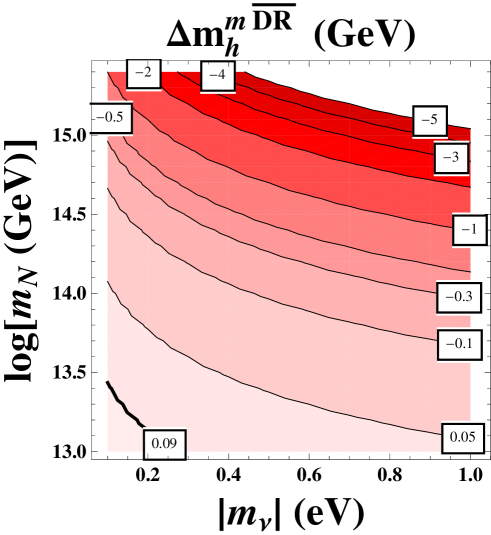
Figure 14: Contour-lines for the Higgs mass corrections from the neutrino/sneutrino sector as a function of the physical Majorana neutrino masses, light $|m_{\nu}|$ and heavy $m_{N}$. The other parameters are fixed to: $A_{\nu}=B_{\nu}=m_{\tilde{L}}=m_{\tilde{R}}=10^{3}\,\,\mathrm{GeV}$, $\tan\beta=5$, $M_{A}=200\,\,\mathrm{GeV}$ and $\mu=200\,\,\mathrm{GeV}$.

The dependence of the mass corrections with the light Majorana neutrino mass is illustrated in the right panel of Fig. 13. The size of the corrections grow with $|m_{\nu}|$, as expected, and can be either positive in the low region, close to $|m_{\nu}|\sim 0.1$ eV, or negative in the high region, close to $|m_{\nu}|\sim 1$ eV.

These same interesting features of the Higgs mass corrections in terms of the two relevant physical Majorana neutrino masses, $m_{N}$ and $m_{\nu}$, are summarized in the contour-plot in Fig. 14. Here we have fixed all the soft parameters, including $m_{\tilde{R}}$, to be at 1 TeV. The contour-lines for fixed $\Delta m_{h}^{\mathrm{m}\overline{\mathrm{DR}}}$ range from positive values around $0.1\,\,\mathrm{GeV}$ in the left lower corner of the plot, corresponding to neutrino mass values of $|m_{\nu}|=0.1-0.3$ eV and $m_{N}=3\times 10^{13}\,\,\mathrm{GeV}$, up to negative values around $-5\,\,\mathrm{GeV}$ in the right upper corner of the plot, corresponding to, for instance, $|m_{\nu}|=1$ eV and $m_{N}=10^{15}\,\,\mathrm{GeV}$. It should be noticed that the contour-line with fixed $\Delta m_{h}^{\mathrm{m}\overline{\mathrm{DR}}}=0.09$ (drawn with a wider black line in this plot) coincides with the prediction for the case where just the gauge part in the self-energies have been included. This means that ’the distance’ of any other contour-line respect to this line represents the difference in the radiative corrections respect to the MSSM prediction.

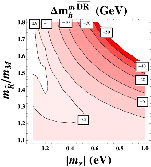
Figure 15: Contour-lines for the Higgs mass corrections from the neutrino/sneutrino sector as a function of the ratio $m_{\tilde{R}}/m_{M}$ and the lightest Majorana neutrino mass $|m_{\nu}|$. The other parameters are fixed to: $m_{M}=10^{14}\,\,\mathrm{GeV}$, $A_{\nu}=B_{\nu}=m_{\tilde{L}}=10^{3}\,\,\mathrm{GeV}$, $\tan\beta=5$, $M_{A}=200\,\,\mathrm{GeV}$ and $\mu=200\,\,\mathrm{GeV}$

We plot in Fig. 15, the contour-lines for fixed $\Delta m_{h}^{\mathrm{m}\overline{\mathrm{DR}}}$ in the less conservative case where $m_{\tilde{R}}$ is close to $m_{M}$. These are displayed as a function of $|m_{\nu}|$ and the ratio $m_{\tilde{R}}/m_{M}$. $m_{M}$ is fixed here to the reference value, $m_{M}=10^{14}$ GeV. For the interval studied here, we see again that the radiative corrections can be negative and as large as tens of GeV in the upper right corner of the plot. For instance, $\Delta m_{h}^{\mathrm{m}\overline{\mathrm{DR}}}=-30\,\,\mathrm{GeV}$ for $m_{M}=10^{14}$ GeV, $|m_{\nu}|=0.6$ eV and $m_{\tilde{R}}/m_{M}=0.7$.

Finally, given our previous simple analytical results of the renormalized self-energies in the seesaw limit, see (100), (101), it is interesting to derive a simple analytical expression for the contribution of the heavy neutrino-sneutrino sector to the one-loop radiatively corrected Higgs mass in the limit of large $m_{M}$. Neglecting in (107) the contributions from $\hat{\Sigma}_{HH}^{\nu/\tilde{\nu}}$ and $\hat{\Sigma}_{hH}^{\nu/\tilde{\nu}}$ one finds,

$$\Delta m_{h}^{\mathrm{m}\overline{\mathrm{DR}}}\simeq-\frac{\hat{\Sigma}_{hh}^{\nu/\tilde{\nu}}(M_{h}^{2})}{2M_{h}}$$ (108)

where $\hat{\Sigma}_{hh}^{\nu/\tilde{\nu}}$ denotes the full corrections to the renormalized Higgs-boson self-energy from the $\nu/\tilde{\nu}$ sector and obtained in the $\mathrm{m}\overline{\mathrm{DR}}$ scheme as described in the present work. We have found that this yields a very good approximation to the full result, i.e. the pole obtained from (107). In a next step in the above expression $\hat{\Sigma}_{hh}^{\nu/\tilde{\nu}}$ has to be replaced by our simplified results in the large $m_{M}$ limit, namely, those in (100b) and (101b), providing the leading ${\cal O}(m_{D}^{0})$ and ${\cal O}(m_{D}^{2})$ contributions. We have compared numerically this approximate $\Delta m_{h}^{\mathrm{m}\overline{\mathrm{DR}}}$ with our full numerical results for large $m_{M}$ in Fig. 12, and found very good agreement, whenever the soft SUSY masses are well below $m_{M}$. In fact, the behaviour with $m_{M}$ of this approximate formula is indistinguishable from the lower line in the left plot of Fig. 12.

We therefore conclude that the use of the previous (108) with

$$\hat{\Sigma}_{hh}^{\nu/\tilde{\nu}}(M_{h}^{2})\simeq\left(\hat{\Sigma}_{hh}^{\mathrm{m}\overline{\mathrm{DR}}}(M_{h}^{2})\right)_{m_{D}^{0}}+\left(\hat{\Sigma}_{hh}^{\mathrm{m}\overline{\mathrm{DR}}}(M_{h}^{2})\right)_{m_{D}^{2}}$$ (109)

as given in (100b) and (101b), respectively, provides an excellent approximation to the full result for large Majorana mass values, $10^{13}\,\,\mathrm{GeV}<m_{M}<10^{15}\,\,\mathrm{GeV}$ and soft masses well below $m_{M}$, $m_{\rm SUSY}\;\raisebox{-3.00003pt}{$\stackrel{{\scriptstyle\displaystyle<}}{{\sim}}$}\;10^{4}\,\,\mathrm{GeV}$. Furthermore, the above simple approximation can also be used for estimates of the differences in the mass correction when applied to the $\overline{\mathrm{DR}}$ scheme versus the $\mathrm{m}\overline{\mathrm{DR}}$ scheme for different choices of the $\mu_{\overline{\mathrm{DR}}}$ scale. For instance, for $m_{M}=10^{14}\,\,\mathrm{GeV}$ and the other parameters set to our reference values as defined in section 4.2, we got small differences of $|(\Delta m_{h}^{\overline{\mathrm{DR}}}-\Delta m_{h}^{\mathrm{m}\overline{\mathrm{DR}}})/M_{h}|<1\%$ for $0.1<\mu_{\overline{\mathrm{DR}}}/m_{M}<1$.

5 Conclusions

In this paper we have presented the one-loop radiative corrections to the renormalized ${\cal CP}$-even Higgs boson self-energies and to the lightest Higgs boson mass from the one-generation neutrino-sneutrino sector within the context of the MSSM-seesaw. The most interesting features in this scenario are that the neutrinos, differently to other fermions, are assumed to be Majorana particles, and that the origin for the light neutrino mass is not as for the other fermions either, but it is instead generated by means of the seesaw mechanism with the addition of heavy right handed neutrinos with a large Majorana mass.

As a first useful result, we have included here the complete set of Feynman rules in this MSSM-seesaw context that are relevant for this work, which to our knowledge are not available in the literature. These include all vertices for the interactions among the Higgs sector and the neutrinos/sneutrinos and for the $Z$ gauge boson and the neutrinos/sneutrinos. These Feynman rules have been presented in terms of all the physical masses and mixing angles of the particles involved, namely, the ${\cal CP}$-even Higgs bosons $h$ and $H$, the ${\cal CP}$-odd Higgs boson $A$, the light and heavy Majorana neutrinos $\nu$ and $N$, their SUSY partners ${\tilde{\nu}}_{\pm}$, ${\tilde{N}}_{\pm}$ and the neutral gauge boson $Z$.

The computation presented here is a full one-loop Feynman diagrammatic one and does not make use of any of the approximations applied in the literature. In particular, we do not use the mass insertion approximation for any of the involved soft mass parameters, nor we neglect the external momentum in the self-energies, which we have found to be relevant for the final computation of the Higgs mass corrections. We have presented our analytical results in terms of the physical neutrinos, sneutrinos, $Z$, and Higgs bosons masses. In addition we have analyzed the role played by the heavy Majorana mass scale $m_{M}$, and emphasized the differences between the Majorana and Dirac neutrino cases.

We have fully analyzed the behavior of the neutrino/sneutrino corrections to the renormalized ${\cal CP}$-even Higgs self-energies with all the involved masses and parameters: $m_{M}$, $\tan\beta$, $M_{A}$, $m_{\tilde{L}}$, $m_{\tilde{R}}$, $A_{\nu}$, $m_{\nu}$ and $B_{\nu}$. Our numerical study of the size of these corrections has been performed over a wide interval for all these parameters, so that our conclusions can be considered as general. From this exhaustive study we have concluded that the most relevant parameters are $m_{M}$, $m_{\nu}$, $m_{\tilde{R}}$ and $B_{\nu}$. In particular, the Majorana mass is by far the most crucial one. In general, we have found sizeable corrections to the self-energies, indeed comparable or even larger than the other relevant one-loop corrections, as the ones from the MSSM top-stop sector, at the highest explored values of $m_{M}$, $m_{\nu}$, $m_{\tilde{R}}$ and $B_{\nu}$. We have explained here the large size of these corrections in terms of the neutrino Yukawa couplings, which are typically large, $Y_{\nu}\sim{\cal O}(1)$ in these seesaw scenarios with heavy Majorana neutrinos. For comparison, we have further included the predictions in two renormalization schemes, the on-shell and the $\overline{\mathrm{DR}}$ schemes, where we have found interesting differences. These differences have been analyzed and explained with the help of simple formulas that are valid in the seesaw limit where $m_{M}$ is much larger than all the other mass scales involved.

The main conclusions on the corrections to the lightest Higgs boson mass are summarized in the contour-plots shown in Figs. 14 and  15. For the most conservative scenario of Fig. 14, where all the soft mass parameters are at the TeV scale, the corrections are positive and smaller than 0.1 GeV if $10^{13}\,\,{\rm GeV}<m_{M}<10^{14}\,\,\mathrm{GeV}$ (or, equivalently, $10^{13}\,\,{\rm GeV}<m_{N}<10^{14}\,\,\mathrm{GeV}$) and $0.1\,\,{\rm eV}<|m_{\nu}|<1$ eV. For larger $m_{M}$ and/or $|m_{\nu}|$ values the corrections change to negative sign and grow in size with these two masses up to values of around $-5\,\,\mathrm{GeV}$ for $m_{M}=10^{15}\,\,\mathrm{GeV}$ and $|m_{\nu}|=1$ eV. For the less conservative scenario of Fig. 15, where the soft mass associated to the right handed neutrino sector, $m_{\tilde{R}}$ is of the order of the Majorana mass scale, we find very large negative corrections, at the right upper corner of the plot, that is for large $m_{M}$ and $m_{\tilde{R}}$, of ${\cal O}(10^{14})\,\,\mathrm{GeV}$, and $|m_{\nu}|$ of ${\cal O}(1)$ eV. For instance, they are around $-30\,\,\mathrm{GeV}$ , for $m_{M}=10^{14}\,\,\mathrm{GeV}$, $m_{\tilde{R}}/m_{M}=0.7$ and $|m_{\nu}|=0.6$ eV. In view of the anticipated experimental precisions at the LHC and the ILC these corrections are very large and should be taken into account if the experimental data indicate the existence of Majorana (s)neutrinos.

In summary, we conclude that the one-loop corrections from heavy Majorana neutrinos to the Higgs boson masses are important in this MSSM-seesaw scenario, and overwhelm by many orders of magnitude the corresponding corrections in the case of Dirac massive neutrinos. These have also been estimated here and are extremely tiny, smaller than $10^{-22}\,\,\mathrm{GeV}$.

Finally, we briefly remark on the interesting and more formal issue of decoupling/non-decoupling effects from the heavy Majorana neutrinos/sneutrinos sector in the low energy MSSM Higgs boson physics. It is clear that our results in the present paper, showing large one-loop corrections $\Delta m_{h}^{\mathrm{m}\overline{\mathrm{DR}}}$ to the $h$ boson mass for large $m_{M}$, suggest that there could be indeed non-decoupling effects from the heavy particles in the low energy MSSM Higgs bosons physics. Particularly suggesting are the numerical results shown in Figs. 12-15 where it is clearly manifested a growing of $\Delta m_{h}^{\mathrm{m}\overline{\mathrm{DR}}}$ with $m_{M}$. Also our simplified analytical results for $\Delta m_{h}^{\mathrm{m}\overline{\mathrm{DR}}}$ in (100b), (101b), (108) and (109) suggest a non-decoupling effect, since the mass correction does not vanish in the asymptotic limit $m_{M}\to\infty$, even for $Y_{\nu}$ (or $m_{D}$) kept fixed. However, we believe that one should not conclude on non-decoupling effects based just on the behaviour of the Higgs mass corrections with $m_{M}$. It is well known that the mass itself is not the proper physical observable to study the decoupling/non-decoupling issue. A more proper tool for that study would be the use of Effective Field Theory techniques, and more concretely the computation of the one-loop effective action by integration in the path integral of the heavy degrees of freedom. An expansion, valid to low external momenta, $p\ll m_{M}$, of the derived 1PI renormalized Green functions with Higgs bosons in the external legs would provide the definite answer to the issue of decoupling/non-decoupling of the heavy $\nu_{R}$, ${\tilde{\nu}}_{R}$, degrees of freedom in the low energy Higgs boson physics. Alternatively one could perform one-loop predictions within the present MSSM-seesaw model for other more proper observables for this issue like, for instance, cross sections involving Higgs particles in the external legs, decay rates of Higgs bosons, etc. The behaviour of these kind of radiative corrections at asymptotically large $m_{M}$ could also be conclusive on this issue. All these proposed studies are extremely interesting but are far beyond the scope of the present work.

Acknowledgements

We thank M. Hirsch and W. Hollik for helpful discussions. The work of S.H. was partially supported by CICYT (grant FPA 2007–66387) and by the Spanish Consolider-Ingenio 2010 Program under grant MultiDark CSD2009-00064. The work of M.H. and A.R.-S. was partially supported by CICYT (grants FPA2006-05423 and FPA2009-09017) and the Comunidad de Madrid project HEPHACOS, S2009/ESP-1473. A.R.-S. thanks the Spanish Ministry of Science and Education for her FPU fellowship Ref. AP2006-02535. The work of S.P. was supported by a Ramón y Cajal contract from MEC (Spain) (PDRYC-2006-000930) and partially by CICYT (grants FPA2006-2315 and FPA2009-09638) and the Comunidad de Aragón project DCYT-DGA E24/2. The work is also supported in part by the European Community’s Marie-Curie Research Training Network under contract MRTN-CT-2006-035505 and also by the Spanish Consolider-Ingenio 2010 Programme CPAN (CSD2007-00042).

Appendix A: New Feynman rules

In this appendix we collect the Feynman rules within the MSSM-seesaw that are relevant for the present work. These correspond to the interactions between the neutrinos and sneutrinos with the MSSM Higgs bosons and between the neutrinos and sneutrinos with the $Z$ gauge bosons. We write all the Feynman rules here in the physical basis. Here $c_{\mathrm{w}}=\cos\theta_{W}$.

	$i\frac{g}{2M_{W}}m_{D}\sin 2\theta\left(\frac{\cos\alpha}{\sin\beta},\frac{\sin\alpha}{\sin\beta},-i\gamma_{5}\cot\beta\right)$
	$-i\frac{g}{2M_{W}}m_{D}\sin 2\theta\left(\frac{\cos\alpha}{\sin\beta},\frac{\sin\alpha}{\sin\beta},-i\gamma_{5}\cot\beta\right)$
	$-i\frac{g}{2M_{W}}m_{M}\sin\theta\cos\theta\left(\frac{\cos\alpha}{\sin\beta},\frac{\sin\alpha}{\sin\beta},-i\gamma_{5}\cot\beta\right)$
	$\frac{ig}{2c_{\mathrm{w}}}\cos^{2}\theta\,\gamma_{\mu}\gamma_{5}$
	$\frac{ig}{2c_{\mathrm{w}}}\sin^{2}\theta\,\gamma_{\mu}\gamma_{5}$

Table 1: Three-point couplings of two Majorana neutrinos to one MSSM Higgs boson and of two Majorana neutrinos to the $Z$ gauge boson.

	$i\frac{g}{4c_{\mathrm{w}}M_{W}\sin\beta}[-4c_{\mathrm{w}}\cos\alpha\,m_{D}^{2}+2c_{\mathrm{w}}\cos\alpha\,m_{D}(A_{\nu}+m_{M}+\mu\tan\alpha\,)\sin 2\theta_{+}$
	$+\frac{M_{W}^{2}}{c_{\mathrm{w}}}\sin\beta\,\sin(\alpha+\beta)\,(1+\cos 2\theta_{+})\,]$
	$-i\frac{g}{4c_{\mathrm{w}}M_{W}\sin\beta}[4c_{\mathrm{w}}\cos\alpha\,m_{D}^{2}+2c_{\mathrm{w}}\cos\alpha\,m_{D}(A_{\nu}+m_{M}+\mu\tan\alpha\,)\sin 2\theta_{+}$
	$-\frac{M_{W}^{2}}{c_{\mathrm{w}}}\sin\beta\,\sin(\alpha+\beta)\,(1-\cos 2\theta_{+})\,]$
	$-i\frac{g}{2c_{\mathrm{w}}M_{W}\sin\beta}[c_{\mathrm{w}}\cos\alpha\,m_{D}(A_{\nu}+m_{M}+\mu\tan\alpha\,)\cos 2\theta_{+}$
	$-\frac{M_{W}^{2}}{c_{\mathrm{w}}}\sin\beta\,\sin(\alpha+\beta)\,\cos\theta_{+}\sin\theta_{+}]$
	$i\frac{g}{4c_{\mathrm{w}}M_{W}\sin\beta}[-4c_{\mathrm{w}}\cos\alpha\,m_{D}^{2}+2c_{\mathrm{w}}\cos\alpha\,m_{D}(A_{\nu}-m_{M}+\mu\tan\alpha\,)\sin 2\theta_{-}$
	$+\frac{M_{W}^{2}}{c_{\mathrm{w}}}\sin\beta\,\sin(\alpha+\beta)\,(1+\cos 2\theta_{-})\,]$
	$-i\frac{g}{4c_{\mathrm{w}}M_{W}\sin\beta}[4c_{\mathrm{w}}\cos\alpha\,m_{D}^{2}+2c_{\mathrm{w}}\cos\alpha\,m_{D}(A_{\nu}-m_{M}+\mu\tan\alpha\,)\sin 2\theta_{-}$
	$-\frac{M_{W}^{2}}{c_{\mathrm{w}}}\sin\beta\,\sin(\alpha+\beta)\,(1-\cos 2\theta_{-})\,]$
	$-\frac{M_{W}^{2}}{c_{\mathrm{w}}}\sin\beta\,\sin(\alpha+\beta)\,\cos\theta_{-}\sin\theta_{-}]$

Table 2: Three-point couplings of two sneutrinos to the Higgs boson $h$. The corresponding couplings to the Higgs boson $H$ are obtained from the ones here by replacing $\cos\alpha\to\sin\alpha\,,\sin\alpha\to-\cos\alpha\,,\sin(\alpha+\beta)\to-\cos(\alpha+\beta)$. All the couplings not shown here vanish.

	$\frac{g}{2c_{\mathrm{w}}}\cos\theta_{+}\cos\theta_{-}\,(p+p^{\prime})_{\mu}$
	$\frac{g}{2c_{\mathrm{w}}}\sin\theta_{+}\sin\theta_{-}\,(p+p^{\prime})_{\mu}$

Table 3: Three-point couplings of two sneutrinos to the $Z$ gauge boson. All the couplings not shown here vanish.

	$i\frac{g}{2M_{W}}\cot\beta\,m_{D}[(A_{\nu}+\mu\tan\beta)\sin(\theta_{-}-\theta_{+})+m_{M}\sin(\theta_{-}+\theta_{+})]$
	$i\frac{g}{2M_{W}}\cot\beta\,m_{D}[-(A_{\nu}+\mu\tan\beta)\cos(\theta_{-}-\theta_{+})+m_{M}\cos(\theta_{-}+\theta_{+})]$

Table 4: Three-point couplings of two sneutrinos to the Higgs boson $A$. All the couplings not shown here vanish.

	$i\frac{g^{2}}{8c_{\mathrm{w}}^{2}M_{W}^{2}\sin^{2}\beta}[4(-\cos^{2}\alpha,\sin^{2}\alpha)c_{\mathrm{w}}^{2}{m_{D}^{2}}+\cos 2\alpha M_{W}^{2}\sin^{2}\beta(1+\cos 2\theta_{+})]$
	$-i\frac{g^{2}}{8c_{\mathrm{w}}^{2}M_{W}^{2}\sin^{2}\beta}[4(\cos^{2}\alpha,\sin^{2}\alpha)c_{\mathrm{w}}^{2}{m_{D}^{2}}(-,+)\cos 2\alpha M_{W}^{2}\sin^{2}\beta(1-\cos 2\theta_{+})]$
	$(+,-)\,i\frac{g^{2}}{4c_{\mathrm{w}}^{2}}\cos 2\alpha\,\cos\theta_{+}\,\sin\theta_{+}$
	$i\frac{g^{2}}{8c_{\mathrm{w}}^{2}M_{W}^{2}\sin^{2}\beta}\sin 2\alpha\,[-2c_{\mathrm{w}}^{2}{m_{D}^{2}}+M_{W}^{2}\sin^{2}\beta\,(1+\cos 2\theta_{+})]$
	$i\frac{g^{2}}{4c_{\mathrm{w}}^{2}}\sin 2\alpha\cos\theta_{+}\sin\theta_{+}$

Table 5: Four-point couplings of two sneutrinos to two ${\cal CP}$-even Higgs bosons. The corresponding couplings for $\tilde{\nu}_{-}$ and $\tilde{N}_{-}$ can be obtained from these by replacing $\theta_{+}\rightarrow\theta_{-}$. All the couplings not shown here vanish

	$i\frac{g^{2}}{8c_{\mathrm{w}}^{2}M_{W}^{2}\sin^{2}\beta}[-4\cos^{2}\beta\,c_{\mathrm{w}}^{2}\,{m_{D}^{2}}+\cos 2\beta\,M_{W}^{2}\,\sin^{2}\beta\,(1+\cos 2\theta_{+})]$
	$-i\frac{g^{2}}{8c_{\mathrm{w}}^{2}M_{W}^{2}\sin^{2}\beta}[4\cos^{2}\beta\,c_{\mathrm{w}}^{2}\,{m_{D}^{2}}-\cos 2\beta\,M_{W}^{2}\,\sin^{2}\beta\,(1-\cos 2\theta_{+})]$
	$i\frac{g^{2}}{4c_{\mathrm{w}}^{2}}\cos 2\beta\,\cos\theta_{+}\,\sin\theta_{+}$
	$i\frac{g^{2}}{2c_{\mathrm{w}}}\cos^{2}\theta_{+}g_{\mu\nu}$
	$i\frac{g^{2}}{2c_{\mathrm{w}}}\sin^{2}\theta_{+}g_{\mu\nu}$

Table 6: Four-point couplings of two sneutrinos to two ${\cal CP}$-odd Higgs bosons and of two sneutrinos to two $Z$ gauge bosons. The corresponding couplings for $\tilde{\nu}_{-}$ and $\tilde{N}_{-}$ can be obtained from these by replacing $\theta_{+}\rightarrow\theta_{-}$. All the couplings not shown here vanish.

Appendix B: Majorana case. One-loop neutrino/sneutrino corrections to the unrenormalized self-energies and tadpoles

In this Appendix we collect all the analytical results for the neutrino and sneutrino one-loop corrections to the Higgs boson tadpoles and unrenormalized self-energies, and to the $Z$ self-energies, within the MSSM-seesaw. The contributions from neutrinos ($\nu$) and sneutrinos (${\tilde{\nu}}$) are presented separately for clearness. Here $c_{\mathrm{w}}=\cos\theta_{W}$.

$${T^{\nu}_{h}} = \frac{g}{16c_{\mathrm{w}}M_{Z}\pi^{2}}\frac{\cos\alpha\sin 2\theta}{\sin\beta}m_{D}(m_{\nu}A_{0}[m_{\nu}^{2}]-m_{N}A_{0}[m_{N}^{2}])$$ (110)

$${T^{\tilde{\nu}}_{h}} = -\frac{g}{64c_{\mathrm{w}}M_{Z}\pi^{2}}\frac{1}{\sin\beta}(A_{0}[m_{\tilde{\nu}_{+}}^{2}](M_{Z}^{2}\cos^{2}\theta_{+}\sin\beta\sin(\alpha+\beta)$$ (111)

$$+m_{D}\mu\sin\alpha\sin 2\theta_{+}+m_{D}\cos\alpha(-2m_{D}+(A_{\nu}+m_{M})\sin 2\theta_{+}))$$

$$+ A_{0}[m_{\tilde{\nu}_{-}}^{2}](M_{Z}^{2}\cos^{2}\theta_{-}\sin\beta\sin(\alpha+\beta)$$

$$+m_{D}\mu\sin\alpha\sin 2\theta_{-}-m_{D}\cos\alpha(2m_{D}-(A_{\nu}-m_{M})\sin 2\theta_{-}))$$

$$- A_{0}[m_{\tilde{N}_{+}}^{2}](-M_{Z}^{2}\sin\beta\sin(\alpha+\beta)\sin^{2}\theta_{+}$$

$$+2m_{D}\cos\alpha(m_{D}+\frac{1}{2}(A_{\nu}+m_{M})\sin 2\theta_{+})+m_{D}\mu\sin\alpha\sin 2\theta_{+})$$

$$- A_{0}[m_{\tilde{N}_{-}}^{2}](-M_{Z}^{2}\sin\beta\sin(\alpha+\beta)\sin^{2}\theta_{-}$$

$$+2m_{D}\cos\alpha(m_{D}+\frac{1}{2}(A_{\nu}-m_{M})\sin 2\theta_{-})+m_{D}\mu\sin\alpha\sin 2\theta_{-}))$$

$${\Sigma_{hh}^{\nu}(p^{2})} = -\frac{g^{2}}{64c_{\mathrm{w}}^{2}M_{Z}^{2}\pi^{2}}\frac{\cos^{2}\alpha\sin^{2}2\theta}{\sin^{2}\beta}\left[2m_{D}^{2}A_{0}[m_{\nu}^{2}]+(2m_{D}^{2}+m_{M}^{2})A_{0}[m_{N}^{2}]\right.$$ (112)

$$+ 4m_{D}^{2}m_{\nu}^{2}B_{0}[p^{2},m_{\nu}^{2},m_{\nu}^{2}]+m_{M}^{2}(m_{\nu}^{2}+m_{\nu}m_{N})B_{0}[p^{2},m_{\nu}^{2},m_{N}^{2}]$$

$$+ 4m_{D}^{2}m_{N}^{2}B_{0}[p^{2},m_{N}^{2},m_{N}^{2}]$$

$$+ \left.p^{2}(2m_{D}^{2}B_{1}[p^{2},m_{\nu}^{2},m_{\nu}^{2}]+m_{M}^{2}B_{1}[p^{2},m_{\nu}^{2},m_{N}^{2}]+2m_{D}^{2}B_{1}[p^{2},m_{N}^{2},m_{N}^{2}])\right]$$

$${\Sigma_{hh}^{\tilde{\nu}}(p^{2})} = \frac{g^{2}}{512c_{\mathrm{w}}^{2}M_{Z}^{2}\pi^{2}\sin^{2}\beta}[-4A_{0}[m_{\tilde{\nu}_{+}}^{2}](-2m_{D}^{2}\cos^{2}\alpha+M_{Z}^{2}\sin^{2}\beta\cos 2\alpha\cos^{2}\theta_{+})$$ (113)

$$- 4A_{0}[m_{\tilde{N}_{+}}^{2}](-2m_{D}^{2}\cos^{2}\alpha+M_{Z}^{2}\sin^{2}\beta\cos 2\alpha\sin^{2}\theta_{+})$$

$$- 4A_{0}[m_{\tilde{\nu}_{-}}^{2}](-2m_{D}^{2}\cos^{2}\alpha+M_{Z}^{2}\sin^{2}\beta\cos 2\alpha\cos^{2}\theta_{-})$$

$$- 4A_{0}[m_{\tilde{N}_{-}}^{2}](-2m_{D}^{2}\cos^{2}\alpha+M_{Z}^{2}\sin^{2}\beta\cos 2\alpha\sin^{2}\theta_{-})]$$

$$+ 2B_{0}[p^{2},m_{\tilde{N}_{+}}^{2},m_{\tilde{\nu}_{+}}^{2}](4m_{D}^{2}\cos^{2}2\theta_{+}\cos^{2}\alpha\,(A_{\nu}+m_{M}+\mu\tan\alpha)^{2}$$

$$+M_{Z}^{2}\sin\beta\sin(\alpha+\beta)(M_{Z}^{2}\sin\beta\sin(\alpha+\beta)\sin^{2}2\theta_{+}$$

$$-2m_{D}\cos\alpha(A_{\nu}+m_{M}+\mu\tan\alpha)\sin 4\theta_{+})$$

$$+ 2B_{0}[p^{2},m_{\tilde{N}_{-}}^{2},m_{\tilde{\nu}_{-}}^{2}](4m_{D}^{2}\cos^{2}2\theta_{-}\cos^{2}\alpha\,(A_{\nu}-m_{M}+\mu\tan\alpha)^{2}$$

$$+M_{Z}^{2}\sin\beta\sin(\alpha+\beta)(M_{Z}^{2}\sin\beta\sin(\alpha+\beta)\sin^{2}2\theta_{-}$$

$$-2m_{D}\cos\alpha(A_{\nu}-m_{M}+\mu\tan\alpha)\sin 4\theta_{-})$$

$$+ 4B_{0}[p^{2},m_{\tilde{N}_{+}}^{2},m_{\tilde{N}_{+}}^{2}](m_{D}\cos\alpha(2m_{D}+\sin 2\theta_{+}(A_{\nu}+m_{M}+\mu\tan\alpha))$$

$$-M_{Z}^{2}\sin\beta\sin(\alpha+\beta)\sin^{2}\theta_{+})^{2}$$

$$+ 4B_{0}[p^{2},m_{\tilde{N}_{-}}^{2},m_{\tilde{N}_{-}}^{2}](m_{D}\cos\alpha(2m_{D}+\sin 2\theta_{-}(A_{\nu}-m_{M}+\mu\tan\alpha))$$

$$-M_{Z}^{2}\sin\beta\sin(\alpha+\beta)\sin^{2}\theta_{-})^{2}$$

$$+ 4B_{0}[p^{2},m_{\tilde{\nu}_{+}}^{2},m_{\tilde{\nu}_{+}}^{2}](m_{D}\cos\alpha(-2m_{D}+\sin 2\theta_{+}(A_{\nu}+m_{M}+\mu\tan\alpha))$$

$$-M_{Z}^{2}\sin\beta\sin(\alpha+\beta)\cos^{2}\theta_{+})^{2}$$

$$+ 4B_{0}[p^{2},m_{\tilde{\nu}_{-}}^{2},m_{\tilde{\nu}_{-}}^{2}](m_{D}\cos\alpha(-2m_{D}+\sin 2\theta_{-}(A_{\nu}-m_{M}+\mu\tan\alpha))$$

$$-M_{Z}^{2}\sin\beta\sin(\alpha+\beta)\cos^{2}\theta_{-})^{2}]$$

The corresponding results for the tadpole $T_{H}$, and the unrenormalized self-energy $\Sigma_{HH}$ are obtained from the above formulas by replacing $\cos\alpha\to\sin\alpha\,,\sin\alpha\to-\cos\alpha\,,\sin(\alpha+\beta)\to-\cos(\alpha+\beta)$.

$${\Sigma_{hH}^{\nu}(p^{2})} = -\frac{g^{2}}{128c_{\mathrm{w}}^{2}M_{Z}^{2}\pi^{2}}\frac{\sin 2\alpha\sin^{2}2\theta}{\sin^{2}\beta}\left[2m_{D}^{2}A_{0}[m_{\nu}^{2}]+(2m_{D}^{2}+m_{M}^{2})A_{0}[m_{N}^{2}]\right.$$ (114)

$$+ 4m_{D}^{2}m_{\nu}^{2}B_{0}[p^{2},m_{\nu}^{2},m_{\nu}^{2}]+m_{M}^{2}(m_{\nu}^{2}+m_{\nu}m_{N})B_{0}[p^{2},m_{\nu}^{2},m_{N}^{2}]$$

$$+ 4m_{D}^{2}m_{N}^{2}B_{0}[p^{2},m_{N}^{2},m_{N}^{2}]]$$

$$+ \left.p^{2}(2m_{D}^{2}B_{1}[p^{2},m_{\nu}^{2},m_{\nu}^{2}]+m_{M}^{2}B_{1}[p^{2},m_{\nu}^{2},m_{N}^{2}]+2m_{D}^{2}B_{1}[p^{2},m_{N}^{2},m_{N}^{2}])\right]$$

$${\Sigma_{hH}^{\tilde{\nu}}(p^{2})} = \frac{g^{2}}{512c_{\mathrm{w}}^{2}M_{Z}^{2}\pi^{2}\sin^{2}\beta}[4A_{0}[m_{\tilde{\nu}_{+}}^{2}]\sin 2\alpha(m_{D}^{2}-M_{Z}^{2}\sin^{2}\beta\cos^{2}\theta_{+})$$ (115)

$$+ 4A_{0}[m_{\tilde{N}_{+}}^{2}]\sin 2\alpha(m_{D}^{2}-M_{Z}^{2}\sin^{2}\beta\sin^{2}\theta_{+})$$

$$+ 4A_{0}[m_{\tilde{\nu}_{-}}^{2}]\sin 2\alpha(m_{D}^{2}-M_{Z}^{2}\sin^{2}\beta\cos^{2}\theta_{-})$$

$$+ 4A_{0}[m_{\tilde{N}_{-}}^{2}]\sin 2\alpha(m_{D}^{2}-M_{Z}^{2}\sin^{2}\beta\sin^{2}\theta_{-})$$

$$+ 2B_{0}[p^{2},m_{\tilde{N}_{+}}^{2},m_{\tilde{\nu}_{+}}^{2}]\times$$

$$(2m_{D}^{2}\cos^{2}2\theta_{+}(-2(A_{\nu}+m_{M})\mu\cos 2\alpha+((A_{\nu}+m_{M})^{2}-\mu^{2})\sin 2\alpha)$$

$$+M_{Z}^{2}\sin\beta(-M_{Z}^{2}\sin\beta\sin(\alpha+\beta)\cos(\alpha+\beta)\sin^{2}2\theta_{+}$$

$$+m_{D}((A_{\nu}+m_{M})\cos(2\alpha+\beta)+\mu\sin(2\alpha+\beta))\sin 4\theta_{+}))$$

$$+ 2B_{0}[p^{2},m_{\tilde{N}_{-}}^{2},m_{\tilde{\nu}_{-}}^{2}]\times$$

$$(2m_{D}^{2}\cos^{2}2\theta_{-}(-2(A_{\nu}-m_{M})\mu\cos 2\alpha+((A_{\nu}-m_{M})^{2}-\mu^{2})\sin 2\alpha)$$

$$+M_{Z}^{2}\sin\beta(-M_{Z}^{2}\sin\beta\sin(\alpha+\beta)\cos(\alpha+\beta)\sin^{2}2\theta_{-}$$

$$+m_{D}((A_{\nu}-m_{M})\cos(2\alpha+\beta)+\mu\sin(2\alpha+\beta))\sin 4\theta_{-}))$$

$$+ 2B_{0}[p^{2},m_{\tilde{N}_{+}}^{2},m_{\tilde{N}_{+}}^{2}](m_{D}^{2}(-2\mu\cos 2\alpha\sin 2\theta_{+}(2m_{D}+(A_{\nu}+m_{M})\sin 2\theta_{+})$$

$$+\sin 2\alpha(4m_{D}^{2}+4m_{D}(A_{\nu}+m_{M})\sin 2\theta_{+}+((A_{\nu}+m_{M})^{2}-\mu^{2})\sin^{2}2\theta_{+}))$$

$$+M_{Z}^{2}m_{D}\sin\beta\sin^{2}\theta_{+}(2\mu\sin(2\alpha+\beta)\sin 2\theta_{+}$$

$$+2(2m_{D}+(A_{\nu}+m_{M})\sin 2\theta_{+})\cos(2\alpha+\beta))$$

$$-M_{Z}^{4}\sin^{2}\beta\sin^{4}\theta_{+}\sin 2(\alpha+\beta))$$

$$+ 2B_{0}[p^{2},m_{\tilde{N}_{-}}^{2},m_{\tilde{N}_{-}}^{2}](-m_{D}^{2}(2\mu\cos 2\alpha\sin 2\theta_{-}(2m_{D}+(A_{\nu}-m_{M})\sin 2\theta_{-})$$

$$-\sin 2\alpha(4m_{D}^{2}+4m_{D}(A_{\nu}-m_{M})\sin 2\theta_{-}+((A_{\nu}-m_{M})^{2}-\mu^{2})\sin^{2}2\theta_{-}))$$

$$+M_{Z}^{2}m_{D}\sin\beta\sin^{2}\theta_{-}(2\mu\sin(2\alpha+\beta)\sin 2\theta_{-}$$

$$+2(2m_{D}+(A_{\nu}-m_{M})\sin 2\theta_{-})\cos(2\alpha+\beta))$$

$$-M_{Z}^{4}\sin^{2}\beta\sin^{4}\theta_{-}\sin 2(\alpha+\beta))$$

$$+ 2B_{0}[p^{2},m_{\tilde{\nu}_{+}}^{2},m_{\tilde{\nu}_{+}}^{2}](-m_{D}^{2}(2\mu\cos 2\alpha\sin 2\theta_{+}(-2m_{D}+(A_{\nu}+m_{M})\sin 2\theta_{+})$$

$$-\sin 2\alpha(4m_{D}^{2}-4m_{D}(A_{\nu}+m_{M})\sin 2\theta_{+}+((A_{\nu}+m_{M})^{2}-\mu^{2})\sin^{2}2\theta_{+}))$$

$$+M_{Z}^{2}m_{D}\sin\beta\cos^{2}\theta_{+}(-2\mu\sin(2\alpha+\beta)\sin 2\theta_{+}$$

$$+2(2m_{D}-(A_{\nu}+m_{M})\sin 2\theta_{+})\cos(2\alpha+\beta))$$

$$-M_{Z}^{4}\sin^{2}\beta\cos^{4}\theta_{+}\sin 2(\alpha+\beta))$$

$$+ 2B_{0}[p^{2},m_{\tilde{\nu}_{-}}^{2},m_{\tilde{\nu}_{-}}^{2}](-m_{D}^{2}(2\mu\cos 2\alpha\sin 2\theta_{-}(-2m_{D}+(A_{\nu}-m_{M})\sin 2\theta_{-})$$

$$-\sin 2\alpha(4m_{D}^{2}-4m_{D}(A_{\nu}-m_{M})\sin 2\theta_{-}+((A_{\nu}-m_{M})^{2}-\mu^{2})\sin^{2}2\theta_{-}))$$

$$+M_{Z}^{2}m_{D}\sin\beta\cos^{2}\theta_{-}(-2\mu\sin(2\alpha+\beta)\sin 2\theta_{-}$$

$$+2(2m_{D}-(A_{\nu}-m_{M})\sin 2\theta_{-})\cos(2\alpha+\beta))$$

$$-M_{Z}^{4}\sin^{2}\beta\cos^{4}\theta_{-}\sin 2(\alpha+\beta))]$$

$${\Sigma_{AA}^{\nu}(M_{A}^{2})} = -\frac{g^{2}}{64c_{\mathrm{w}}^{2}M_{Z}^{2}\pi^{2}}\frac{\cos^{2}\beta\sin^{2}2\theta}{\sin^{2}\beta}[2m_{D}^{2}A_{0}[m_{\nu}^{2}]+(2m_{D}^{2}+m_{M}^{2})A_{0}[m_{N}^{2}]$$

$$+ m_{M}^{2}(m_{\nu}^{2}-m_{\nu}m_{N})B_{0}[M_{A}^{2},m_{\nu}^{2},m_{N}^{2}]$$

$$+ M_{A}^{2}(2m_{D}^{2}(B_{1}[M_{A}^{2},m_{\nu}^{2},m_{\nu}^{2}]+B_{1}[M_{A}^{2},m_{N}^{2},m_{N}^{2}])+m_{M}^{2}B_{1}[M_{A}^{2},m_{\nu}^{2},m_{N}^{2}])]$$

$${\Sigma_{AA}^{\tilde{\nu}}(M_{A}^{2})} = \frac{g^{2}}{256c_{\mathrm{w}}^{2}M_{Z}^{2}\pi^{2}}\frac{1}{\sin^{2}\beta}[A_{0}[m_{\tilde{\nu}_{+}}^{2}](4m_{D}^{2}\cos^{2}\beta-2M_{Z}^{2}\cos 2\beta\sin^{2}\beta\cos^{2}\theta_{+})$$ (117)

$$+ A_{0}[m_{\tilde{N}_{+}}^{2}](4m_{D}^{2}\cos^{2}\beta-2M_{Z}^{2}\cos 2\beta\sin^{2}\beta\sin^{2}\theta_{+})$$

$$+ A_{0}[m_{\tilde{\nu}_{-}}^{2}](4m_{D}^{2}\cos^{2}\beta-2M_{Z}^{2}\cos 2\beta\sin^{2}\beta\cos^{2}\theta_{-})$$

$$+ A_{0}[m_{\tilde{N}_{-}}^{2}](4m_{D}^{2}\cos^{2}\beta-2M_{Z}^{2}\cos 2\beta\sin^{2}\beta\sin^{2}\theta_{-})$$

$$+ 4m_{D}^{2}\left[B_{0}[M_{A}^{2},m_{\tilde{\nu}_{+}}^{2},m_{\tilde{\nu}_{-}}^{2}](\mu\sin\beta\sin(\theta_{-}-\theta_{+})\right.$$

$$+\cos\beta(A_{\nu}\sin(\theta_{-}-\theta_{+})-m_{M}\sin(\theta_{-}+\theta_{+})))^{2}$$

$$+ B_{0}[M_{A}^{2},m_{\tilde{N}_{+}}^{2},m_{\tilde{N}_{-}}^{2}](\mu\sin\beta\sin(\theta_{-}-\theta_{+})$$

$$+\cos\beta(A_{\nu}\sin(\theta_{-}-\theta_{+})+m_{M}\sin(\theta_{-}+\theta_{+})))^{2}$$

$$+ B_{0}[M_{A}^{2},m_{\tilde{N}_{-}}^{2},m_{\tilde{\nu}_{+}}^{2}](\mu\sin\beta\cos(\theta_{-}-\theta_{+})$$

$$+\cos\beta(A_{\nu}\cos(\theta_{-}-\theta_{+})-m_{M}\cos(\theta_{-}+\theta_{+})))^{2}$$

$$+ B_{0}[M_{A}^{2},m_{\tilde{N}_{+}}^{2},m_{\tilde{\nu}_{-}}^{2}](\mu\sin\beta\cos(\theta_{-}-\theta_{+})$$

$$\left.+\cos\beta(A_{\nu}\cos(\theta_{-}-\theta_{+})+m_{M}\cos(\theta_{-}+\theta_{+})))^{2}\right]]$$

$${\Sigma_{ZZ}^{\nu}(M_{Z}^{2})} = -\frac{g^{2}}{32c_{\mathrm{w}}^{2}\pi^{2}}\left[\cos^{4}\theta A_{0}[m_{\nu}^{2}]+\frac{1}{2}(3+\cos 2\theta)\sin^{2}\theta A_{0}[m_{N}^{2}]\right.$$ (118)

$$+ 2\cos^{4}\theta\left(m_{\nu}^{2}B_{0}[M_{Z}^{2},m_{\nu}^{2},m_{\nu}^{2}]-B_{00}[M_{Z}^{2},m_{\nu}^{2},m_{\nu}^{2}]+\frac{M_{Z}^{2}}{2}B_{1}[M_{Z}^{2},m_{\nu}^{2},m_{\nu}^{2}]\right)$$

$$+ 2\sin^{4}\theta\left(m_{N}^{2}B_{0}[M_{Z}^{2},m_{N}^{2},m_{N}^{2}]-B_{00}[M_{Z}^{2},m_{N}^{2},m_{N}^{2}]+\frac{M_{Z}^{2}}{2}B_{1}[M_{Z}^{2},m_{N}^{2},m_{N}^{2}]\right)$$

$$+ \frac{1}{2}\sin^{2}2\theta\left(m_{\nu}(m_{\nu}+m_{N})B_{0}[M_{Z}^{2},m_{\nu}^{2},m_{N}^{2}]-2B_{00}[M_{Z}^{2},m_{\nu}^{2},m_{N}^{2}]\right.$$

$$\left.\left.+M_{Z}^{2}B_{1}[M_{Z}^{2},m_{\nu}^{2},m_{N}^{2}]\right)\right]$$

$${\Sigma_{ZZ}^{\tilde{\nu}}(M_{Z}^{2})} = \frac{g^{2}}{64c_{\mathrm{w}}^{2}\pi^{2}}\Big{[}A_{0}[m_{\tilde{\nu}_{-}}^{2}]\cos^{2}\theta_{-}+A_{0}[m_{\tilde{\nu}_{+}}^{2}]\cos^{2}\theta_{+}$$ (119)

$$+ A_{0}[m_{\tilde{N}_{-}}^{2}]\sin^{2}\theta_{-}+A_{0}[m_{\tilde{N}_{+}}^{2}]\sin^{2}\theta_{+}$$

$$- 4(B_{00}[M_{Z}^{2},m_{\tilde{\nu}_{+}}^{2},m_{\tilde{\nu}_{-}}^{2}]\cos^{2}\theta_{-}\cos^{2}\theta_{+}+B_{00}[M_{Z}^{2},m_{\tilde{N}_{-}}^{2},m_{\tilde{\nu}_{+}}^{2}]\cos^{2}\theta_{+}\sin^{2}\theta_{-}$$

$$+ B_{00}[M_{Z}^{2},m_{\tilde{N}_{+}}^{2},m_{\tilde{\nu}_{-}}^{2}]\cos^{2}\theta_{-}\sin^{2}\theta_{+}+B_{00}[M_{Z}^{2},m_{\tilde{N}_{+}}^{2},m_{\tilde{N}_{-}}^{2}]\sin^{2}\theta_{-}\sin^{2}\theta_{+})\Big{]}$$

The definitions of the loop functions $A_{0}$, $B_{0}$, $B_{1}$ and $B_{00}$ appearing in this and the next appendices can be found, for instance, in  Ref. [45] (where $B_{00}=B_{22}$).

Appendix C: Dirac case. One-loop contributions from neutrinos and sneutrinos to the renormalized $h$ Higgs boson self-energy

We present here the result for the one-loop corrections from neutrinos ($\nu$) and sneutrinos (${\tilde{\nu}}$) to the renormalized $hh$ self-energy in the case of Dirac neutrinos, obtained in the $\overline{\rm{DR}}$ scheme. Here $c_{\mathrm{w}}=\cos\theta_{W}$.

$$\hat{\Sigma}_{hh}^{\nu}(p^{2})_{\mathrm{Dirac}} = \frac{g^{2}}{32c_{\mathrm{w}}^{2}M_{Z}^{2}\pi^{2}}\Big{\{}A_{0}[m_{D}^{2}]\,(\sin^{2}(\alpha+\beta)M_{Z}^{2}$$ (120)

$$+\frac{1}{\sin\beta}(\sin(2\alpha-3\beta)+3\sin(2\alpha-\beta)-2\sin\beta))m_{D}^{2}$$

$$+ \sin^{2}(\alpha+\beta)M_{Z}^{2}(m_{D}^{2}B_{0}[M_{Z}^{2},m_{D}^{2},m_{D}^{2}]$$

$$-2B_{00}[M_{Z}^{2},m_{D}^{2},m_{D}^{2}]+M_{Z}^{2}B_{1}[M_{Z}^{2},m_{D}^{2},m_{D}^{2}])$$

$$- 2\frac{\cos^{2}\alpha}{\sin^{2}\beta}(2m_{D}^{4}B_{0}[p^{2},m_{D}^{2},m_{D}^{2}]+p^{2}B_{1}[p^{2},m_{D}^{2},m_{D}^{2}])$$

$$+ 2M_{A}^{2}m_{D}^{2}\frac{\cos^{2}(\alpha-\beta)\cos^{2}\beta}{\sin^{2}\beta}B_{1}[M_{A}^{2},m_{D}^{2},m_{D}^{2}]\Big{\}}$$

$$\hat{\Sigma}_{hh}^{\tilde{\nu}}(p^{2})_{\mathrm{Dirac}} = -\frac{g^{2}}{256c_{\mathrm{w}}^{2}M_{Z}^{2}\pi^{2}}\Bigg{\{}A_{0}[m_{\tilde{\nu}_{1}}^{2}]\Big{[}8M_{Z}^{2}\sin^{2}(\alpha+\beta)\cos^{2}{\tilde{\theta}}+2m_{D}\frac{\sin(\alpha-\beta)\sin 2{\tilde{\theta}}}{\sin\beta}\times$$ (121)

$$\qquad(\mu(3\sin\alpha-\sin(\alpha-2\beta))+A_{\nu}(3\cos\alpha+\cos(\alpha-2\beta)))\Big{]}$$

$$+ A_{0}[m_{\tilde{\nu}_{2}}^{2}]\Big{[}8M_{Z}^{2}\sin^{2}(\alpha+\beta)\sin^{2}{\tilde{\theta}}-2m_{D}\frac{\sin(\alpha-\beta)\sin 2{\tilde{\theta}}}{\sin\beta}\times$$

$$\qquad(\mu(3\sin\alpha-\sin(\alpha-2\beta))+A_{\nu}(3\cos\alpha+\cos(\alpha-2\beta)))\Big{]}$$

$$- \frac{1}{16}\frac{1}{\sin^{2}\beta}B_{0}[p^{2},m_{\tilde{\nu}_{1}}^{2},m_{\tilde{\nu}_{1}}^{2}]\Big{[}2(8m_{D}^{2}-M_{Z}^{2})\cos\alpha$$

$$\qquad+2M_{Z}^{2}(\cos(\alpha+2\beta)-2\cos 2{\tilde{\theta}}\sin\beta\sin(\alpha+\beta))$$

$$\qquad-8m_{D}\sin 2{\tilde{\theta}}\cos\alpha(A_{\nu}+\mu\tan\alpha)\Big{]}^{2}$$

$$- \frac{1}{16}\frac{1}{\sin^{2}\beta}B_{0}[p^{2},m_{\tilde{\nu}_{2}}^{2},m_{\tilde{\nu}_{2}}^{2}]\Big{[}2(8m_{D}^{2}-M_{Z}^{2})\cos\alpha$$

$$\qquad+2M_{Z}^{2}(\cos(\alpha+2\beta)+2\cos 2{\tilde{\theta}}\sin\beta\sin(\alpha+\beta))$$

$$\qquad+8m_{D}\sin 2{\tilde{\theta}}\cos\alpha(A_{\nu}+\mu\tan\alpha)\Big{]}^{2}$$

$$- \frac{1}{8}\frac{1}{\sin^{2}\beta}B_{0}[p^{2},m_{\tilde{\nu}_{2}}^{2},m_{\tilde{\nu}_{1}}^{2}]\Big{[}-4M_{Z}^{2}\sin 2{\tilde{\theta}}\sin\beta\sin(\alpha+\beta)$$

$$\qquad+8m_{D}\cos 2{\tilde{\theta}}\cos\alpha(A_{\nu}+\mu\tan\alpha)\Big{]}^{2}$$

$$+ 8m_{D}^{2}\cos^{2}(\alpha-\beta)\cot^{2}\beta\,B_{0}[M_{A}^{2},m_{\tilde{\nu}_{2}}^{2},m_{\tilde{\nu}_{1}}^{2}]\,(A_{\nu}+\mu\tan\beta)^{2}$$

$$- 8M_{Z}^{2}\sin^{2}(\alpha+\beta)\left(2\cos^{4}{\tilde{\theta}}B_{00}[M_{Z}^{2},m_{\tilde{\nu}_{1}}^{2},m_{\tilde{\nu}_{1}}^{2}]+2\sin^{4}{\tilde{\theta}}B_{00}[M_{Z}^{2},m_{\tilde{\nu}_{2}}^{2},m_{\tilde{\nu}_{2}}^{2}]\right.$$

$$\left.+\sin^{2}2{\tilde{\theta}}B_{00}[M_{Z}^{2},m_{\tilde{\nu}_{2}}^{2},m_{\tilde{\nu}_{1}}^{2}]\right)\Bigg{\}}$$

References

- [1] K. Nakamura et al. (Particle Data Group), J. Phys. G 37, 075021 (2010).
-
[2]
H.P. Nilles,
Phys. Rep. 110 (1984) 1;
H.E. Haber and G.L. Kane, Phys. Rep. 117 (1985) 75;
R. Barbieri, Riv. Nuovo Cim. 11 (1988) 1. -
[3]
P. Minkowski,
Phys. Lett. B 67 (1977) 421;
M. Gell-Mann, P. Ramond and R. Slansky, in Complex Spinors and Unified Theories eds. P. Van. Nieuwenhuizen and D. Z. Freedman, Supergravity (North-Holland, Amsterdam, 1979), p.315 [Print-80-0576 (CERN)];
T. Yanagida, in Proceedings of the Workshop on the Unified Theory and the Baryon Number in the Universe, eds. O. Sawada and A. Sugamoto (KEK, Tsukuba, 1979), p.95;
S. Glashow, in Quarks and Leptons, eds. M. Lévy et al., Plenum Press, New York U.S.A. (1980), p.707;
R. N. Mohapatra and G. Senjanović, Phys. Rev. Lett. 44 (1980) 912. - [4] J. Gunion and H. Haber, Nucl. Phys. B 272 (1986) 1 [Erratum-ibid. B 402 (1993) 567].
- [5] M. Fukugita and T. Yanagida, Phys. Lett. B 174 (1986) 45.
-
[6]
For a general overview and selected references therein, see, for instance:
M. Raidal et al., Eur. Phys. J. C 57 (2008) 13 [arXiv:0801.1826 [hep-ph]]. -
[7]
F. Borzumati and A. Masiero,
Phys. Rev. Lett. 57 (1986) 961;
J. Hisano, T. Moroi, K. Tobe, M. Yamaguchi and T. Yanagida, Phys. Lett. B 357 (1995) 579; [arXiv:hep-ph/9501407];
J. Hisano, T. Moroi, K. Tobe and M. Yamaguchi, Phys. Rev. D 53 (1996) 2442 [arXiv:hep-ph/9510309];
J. Ellis, J. Hisano, M. Raidal and Y. Shimizu, Phys. Rev. D 66 (2002) 115013 [arXiv:hep-ph/0206110];
E. Arganda and M. Herrero, Phys. Rev. D 73 (2006) 055003 [arXiv:hep-ph/0510405].;
S. Antusch, E. Arganda, M. J. Herrero and A. M. Teixeira, JHEP 0611, 090 (2006) [arXiv:hep-ph/0607263]. -
[8]
E. Arganda, M. J. Herrero and A. M. Teixeira,
JHEP 0710, 104 (2007)
[arXiv:0707.2955 [hep-ph]];
E. Arganda, M. J. Herrero and J. Portoles, JHEP 0806, 079 (2008) [arXiv:0803.2039 [hep-ph]].;
M. J. Herrero, J. Portoles and A. M. Rodriguez-Sanchez, Phys. Rev. D 80, 015023 (2009) [arXiv:0903.5151 [hep-ph]]. -
[9]
J. Ellis, J. Hisano, M. Raidal and Y. Shimizu,
Phys. Lett. B 528 (2002) 86
[arXiv:hep-ph/0111324];
I. Masina, Nucl. Phys. B 671 (2003) 432 [arXiv:hep-ph/0304299];
Y. Farzan and M. E. Peskin, Phys. Rev. D 70 (2004) 095001 [arXiv:hep-ph/0405214]. - [10] Y. Grossman and H. Haber, Phys. Rev. Lett. 78 (1997) 3438 [arXiv:hep-ph/9702421].
- [11] A. Dedes, H. Haber and J. Rosiek, JHEP 0711 (2007) 059 [arXiv:0707.3718 [hep-ph]].
- [12] J. Cao and J. M. Yang, Phys. Rev. D 71 (2005) 111701 [arXiv:hep-ph/0412315].
- [13] Y. Farzan, JHEP 0502 (2005) 025 [arXiv:hep-ph/0411358].
-
[14]
S. K. Kang, A. Kato, T. Morozumi and N. Yokozaki,
Phys. Rev. D 81, 016011 (2010)
[arXiv:0909.2484 [hep-ph]];
S. K. Kang, T. Morozumi and N. Yokozaki, arXiv:1005.1354 [hep-ph]. -
[15]
A. Brignole,
Phys. Lett. B 281 (1992) 284;
P. Chankowski, S. Pokorski and J. Rosiek, Phys. Lett. B 286 (1992) 307;
A. Dabelstein, Nucl. Phys. B 456 (1995) 25 [arXiv:hep-ph/9503443]; - [16] G. Degrassi, S. Heinemeyer, W. Hollik, P. Slavich and G. Weiglein, Eur. Phys. J. C 28 (2003) 133 [arXiv:hep-ph/0212020].
-
[17]
S. Martin,
Phys. Rev. D 75 (2007) 055005
[arXiv:hep-ph/0701051];
R. Harlander, P. Kant, L. Mihaila and M. Steinhauser, Phys. Rev. Lett. 100 (2008) 191602 [Phys. Rev. Lett. 101 (2008) 039901] [arXiv:0803.0672 [hep-ph]]; arXiv:1005.5709 [hep-ph]. -
[18]
G. Aad et al. [The ATLAS Collaboration],
arXiv:0901.0512;
G. Bayatian et al. [CMS Collaboration], J. Phys. G 34 (2007) 995. - [19] K. Cranmer, Y. Fang, B. Mellado, S. Paganis, W. Quayle and S. Wu, arXiv:hep-ph/0401148.
- [20] S. Abdullin et al., Eur. Phys. J. C 39S2 (2005) 41.
- [21] S. Gennai, S. Heinemeyer, A. Kalinowski, R. Kinnunen, S. Lehti, A. Nikitenko and G. Weiglein, Eur. Phys. J. C 52 (2007) 383 [arXiv:0704.0619 [hep-ph]].
- [22] V. Büscher and K. Jakobs, Int. J. Mod. Phys. A 20 (2005) 2523 [arXiv:hep-ph/0504099].
- [23] M. Schumacher, Czech. J. Phys. 54 (2004) A103; arXiv:hep-ph/0410112.
-
[24]
J. Aguilar-Saavedra et al.,
TESLA TDR Part 3:
“Physics at an Linear Collider”,
arXiv:hep-ph/0106315,
see:
http://tesla.desy.de/new_pages/TDR_CD/start.html;
K. Ackermann et al., DESY-PROC-2004-01, prepared for 4th ECFA / DESY Workshop on Physics and Detectors for a 90-GeV to 800-GeV Linear e+ e- Collider, Amsterdam, The Netherlands, 1-4 Apr 2003. - [25] T. Abe et al. [American Linear Collider Working Group Collaboration], arXiv:hep-ex/0106056.
- [26] K. Abe et al. [ACFA Linear Collider Working Group Collaboration], arXiv:hep-ph/0109166.
- [27] S. Heinemeyer et al., arXiv:hep-ph/0511332.
-
[28]
[LHC / ILC Study Group], G. Weiglein et al.,
Phys. Rept. 426 (2006) 47
[arXiv:hep-ph/0410364];
A. De Roeck et al., Eur. Phys. J. C 66 (2010) 525 [arXiv:0909.3240 [hep-ph]]. - [29] K. Desch, E. Gross, S. Heinemeyer, G. Weiglein and L. Zivkovic, JHEP 0409 (2004) 062 [arXiv:hep-ph/0406322].
- [30] J. Gunion, H. Haber, G. Kane and S. Dawson, The Higgs Hunter’s Guide, Addison-Wesley, 1990.
- [31] M. Frank, S. Heinemeyer, W. Hollik and G. Weiglein, arXiv:hep-ph/0202166.
- [32] A. Freitas and D. Stockinger, Phys. Rev. D 66 (2002) 095014 [arXiv:hep-ph/0205281].
- [33] M. Frank, T. Hahn, S. Heinemeyer, W. Hollik, H. Rzehak and G. Weiglein, JHEP 0702 (2007) 047 [arXiv:hep-ph/0611326].
- [34] M. Frank, PhD thesis: “Radiative Corrections in the Higgs Sector of the MSSM with Violation”, University of Karlsruhe, 2002, ISBN 3-937231-01-3.
- [35] J. Collins, F. Wilczek and A. Zee, Phys. Rev. D 18 (1978) 242.
- [36] P. Nason, S. Dawson and R. K. Ellis, Nucl. Phys. B 327 (1989) 49 [Erratum-ibid. B 335 (1990) 260].
-
[37]
J. Küblbeck, M. Böhm and A. Denner,
Comput. Phys. Commun. 60 (1990) 165;
T. Hahn, Comput. Phys. Commun. 140 (2001) 418 [arXiv:hep-ph/0012260];
T. Hahn and C. Schappacher, Comput. Phys. Commun. 143 (2002) 54 [arXiv:hep-ph/0105349]. - [38] T. Hahn and M. Pérez-Victoria, Comput. Phys. Commun. 118 (1999) 153 [arXiv:hep-ph/9807565].
-
[39]
W. Siegel,
Phys. Lett. B 84 (1979) 193;
D. Capper, D. Jones, and P. van Nieuwenhuizen, Nucl. Phys. B 167 (1980) 479. - [40] D. Stöckinger, JHEP 0503 (2005) 076 [arXiv:hep-ph/0503129].
- [41] W. Hollik and D. Stöckinger, Phys. Lett. B 634 (2006) 63 [arXiv:hep-ph/0509298].
-
[42]
For reviews on radiative corrections to MSSM Higgs
boson masses, see, for instance,
A. Djouadi,
Phys. Rept. 459 (2008) 1
[arXiv:hep-ph/0503173];
S. Heinemeyer, Int. J. Mod. Phys. A 21 2659 (2006) [arXiv:hep-ph/0407244], and references therein. - [43] S. Heinemeyer, W. Hollik and G. Weiglein, Comput. Phys. Commun. 124 (2000) 76 [arXiv:hep-ph/9812320]; see: www.feynhiggs.de .
- [44] S. Heinemeyer, W. Hollik and G. Weiglein, Eur. Phys. J. C 9 (1999) 343 [arXiv:hep-ph/9812472].
-
[45]
W. Beenakker,
PhD thesis: “Electroweak Corrections: Techniques and Applications”,
University of Leiden, 1989;
W. Hollik, ”Precision Tests of the Electroweak Theory, Part 1”. Lectures given at the CERN-JINR School of Physics 1989. CERN-TH-5661/90