Phase-space description of the magneto-optical trap

Abstract

An exhaustive kinetic model for the atoms in a 1D Magneto-Optical Trap is derived, without any approximations. It is shown that the atomic density is described by a Vlasov-Fokker-Planck equation, coupled with two simple differential equations describing the trap beam propagation. The analogy of such a system with plasmas is discussed. This set of equations is then simplified through some approximations, and it is shown that corrective terms have to be added to the models usually used in this context.

1 Introduction

The magneto-optical trap (MOT) is the primary tool to cool atoms. The development of this technique led to spectacular breakthroughs in experimental quantum physics: MOTs are the first step in the realization of optical lattices lattices , cold molecules molecules , or Bose-Einstein condensates BEC . But the MOT is also an interesting object per se. It produces a cloud of cold atoms, the physics of which is complex. In particular, spatio-temporal instabilities of this cloud are commonly observed wilkowski2000 ; labeyrie2006 . Several models with different approaches have been proposed to describe these dynamics, and to identify the mechanisms leading to instabilities. Unfortunately, none of these models gives a satisfying description of the observed dynamics. In wilkowski2000 , a very simple model allowed to describe experimentally observed instabilities. This model, improved in hennequin2004 , predicted another type of instabilities, which were effectively observed in distefano2003 ; distefano2004 . However, the agreement between the model and the experiments was only qualitative. Moreover, it concerned the particular case where the counterpropagating trap beams are obtained by retro-reflection, i.e. a global asymmetry is introduced in the trap.

Recently, it has been proposed to describe the symmetric MOT, with all trap beams which are independent, as a weakly damped plasma labeyrie2006 ; pohl2006 . Indeed, the cloud of cold atoms in a MOT is a confined dilute object with long-range interactions, as in plasmas walker1990 ; pruvost2000 . This model predicted the existence of instabilities above a relatively high threshold, so that instabilities should exist only in large MOTs. This seems in contradiction with the observations related in hennequin2004 . Moreover, no direct comparison with the experimental temporal regimes allowed validating this model. More recently, a more complete description was derived using the methods of waves and oscillations in plasmas, leading to interesting predictions mendonca2008 . But as in the previous case, this study is based upon intermediate well-established results, valid only in specific cases (e.g. a low beam intensity or a negligible viscosity). These conditions do not correspond in general to the experimental situations, and indeed, these results were not compared to experimental results.

It appears from these numerous works that a reference model for MOT atom clouds lacks. Such a model should be as general as possible, and should at least describe the usual experimental situations. In particular, such approximations as the low saturation limit should not be done a priori. Another interest of such a model is that it could help in determining precisely the analogies between MOT atom clouds and other systems, such as plasmas.

The present work is a first step towards such a model. Its aim is to build a model, with the least possible hypotheses and approximations, of a 1D symmetric MOT. The resulting set of equations describes as precisely as possible the dynamics of atoms inside a 1D MOT, and constitutes a basis model. If simplifications are necessary, approximations should be applied on this model, a posteriori.

The paper is organized as follows: section 2 defines the bases of the model, while in section 3, we show that the dynamics of the MOT phase space density can be described by a Vlasov-Fokker-Planck equation with two relaxation processes. In section 4, we derive the different terms of this equation of evolution as a function of the usual experimental parameters. In section 5, we establish the equations of propagation of the trapping beams. We obtain a set of coupled equations fully describing our system, in the general case. This set of equation can be solved numerically to obtain solutions of the general system. However, to have a better understanding of the MOT, it is interesting to go further in the analytical approach, simplifying a posteriori the model, as discussed above. This is done in section 6, where we examine an approximation for the atomic response.

2 Definition of the model

As discussed above, we consider here a 1D configuration. Two counterpropagating laser beams with opposite circular polarizations interact with the atoms, as sketched on Figure 1a. The beam with the $\sigma^{-}$ polarization comes from the negative abscissa, and is denoted by the minus sign (intensity $I_{-}(x,t)$, wave vector $k_{-}$). In the same way, the beam with the $\sigma^{+}$ polarization comes from the positive abscissa (intensity $I_{+}(x,t)$, wave vector $k_{+}$). Forces originate from the exchange of momentum between the atoms and the electromagnetic field. We consider here that the atoms are the simplest ones for which the magneto-optical trapping is possible. The laser frequency $\omega_{L}$ is tuned in the vicinity of a $J=0\rightarrow J^{\prime}=1$ transition with a frequency $\omega_{0}$ (Fig. 1b).

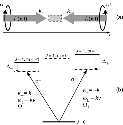
Figure 1: Sketch of the 1D system considered here. a) the two contrapropagating beams have opposite circular polarizations. b) The laser beams interact with “three-level” atoms on a $J=0\rightarrow J^{\prime}=1$ transition, the degeneracy of which is lifted by an inhomogeneous magnetic field. $\Omega_{\pm}$ are the Rabi frequencies associated with the beams; $\Delta_{\pm}$ are the effective detunings (see section 4.1).

In the 2D phase space, a point has the coordinates $\left(x,p\right)$, where $x$ is the position and $p$ is the momentum. To describe the cloud of cold atoms, we introduce the phase space density $\rho\left(x,p,t\right)$. Formally, the complete atomic system is described by a phase space density including both the hot and the cold atoms. However, laser cooling acts only in a limited region of space, typically the intersection of the laser beams, and for moderate velocities. As a consequence, the surrounding hot atoms are considered as a large reservoir which remain in a thermal equilibrium at room temperature. In the following, we neglect the action of the cold atoms on the hot background. These approximations lead to a huge simplification in the description of the collisions. Thus, to describe the cold atom dynamics, we have just to derive the equation of evolution of $\rho\left(x,p,t\right)$ from the basic principles of atomic physics. This approach allows us to go beyond the Wieman description of multiple scattering in terms of absorption cross sections walker1990 ; sesko1991 . $\rho\left(x,p,t\right)$ influences the propagation of the trapping beams, and reciprocally the modification in the beam intensities changes the evolution of the phase space density. Thus, we expect to obtain a system of coupled nonlinear differential equations. As our aim is to build a theoretical frame in which most of the experimental situations can be explored, we limit as much as possible the initial approximations. In particular, we do not restrict our study to the low saturation limit, as in mendonca2008 .

To derive the system of coupled equations, we proceed in two steps. We first assume that we know the intensities of the beams everywhere in the sample, and we derive the equation of evolution of the density in phase space (section 3 et 4). Then, we write the equations of propagation of the beams assuming that we know the atomic density in phase space (section 5).

3 Evolution of the phase space density

To derive the equation of evolution of the phase space density $\rho\left(x,p,t\right)$, we consider an elementary cell centered in $\left(x_{0},p_{0}\right)$, with dimensions $\delta x$ and $\delta p$. The number of atoms contained in this cell is $N(t)=\rho\left(x_{0},p_{0},t\right)\delta x\,\delta p$, where we assume that $\delta x$ and $\delta p$ have been chosen small enough to neglect higher order corrections. The variations of $N$ between $t$ and $t+\delta t$ are governed by three distinct phenomena: (i) an atom is kicked in or out by a collision with the hot background gas or (ii) an atom crosses the border of the cell because of the evolution of either its position or (iii) its momentum. The simultaneous change in position and in momentum would lead to second order terms in $\delta t$, which are neglected.

The collisional processes lead to two terms, one for losses and one for gains :

$$\delta N_{coll}=-\frac{N\,\delta t}{\tau}+\lambda\,\delta x\,\delta p\,\delta t$$ (1)

where $\tau$ is the mean time interval between two collisions with the hot atoms. The source term $\lambda$ is due to the collisions between two hot atoms that tend to restore the Maxwell-Boltzmann distribution for the phase space density (uniform in $x$, gaussian in $p$). A contribution from the collisions between cold atoms could also be considered but, in the conditions where instabilities are observed in a MOT, this last contribution can be neglected.

The second mechanism is the variation of $N$ due to the velocity of the atoms. As depicted in Fig. 2a, the atoms that cross the borders in $x_{0}\pm\delta x/2$ with a velocity $p_{0}/m$, where $m$ is the atomic mass, between $t$ and $t+\delta t$ are those in the close vicinity of that border. The area of these zones is simply $\delta p\,p_{0}\,\delta t/m$. The variation $\delta N_{x}$ in $N$ due to the velocity of the atoms can then be written:

$$\delta N_{x} = \frac{\delta p\,p_{0}\,\delta t}{m}\left[\rho\left(x_{0}-\frac{\delta x}{2},p_{0},t\right)-\rho\left(x_{0}+\frac{\delta x}{2},p_{0},t\right)\right]$$ (2)

$$= -\left(\delta x\,\delta p\,\delta t\right)\,\frac{p_{0}}{m}\,\frac{\partial}{\partial x}\rho\left(x_{0},p_{0},t\right)$$

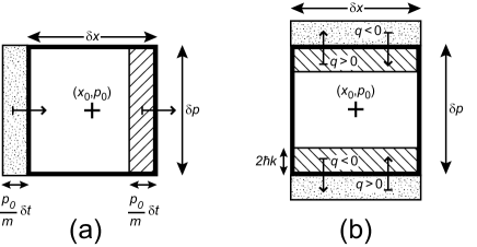
Figure 2: Modification of the number of atoms contained in the elementary cell due to the evolution of (a) the position and (b) the momentum. The dashed regions contribute to losses, while dotted regions contribute to gains. In (a), all the atoms in the indicated regions will cross a boundary (we assume that $p_{0}>0$), and the areas are proportional to $\delta t$. In (b), a small fraction of the atoms, proportional to $\delta t$, will receive a momentum kick. We have to consider separately the momentum kicks with $q>0$ and those with $q<0$.

The last mechanism that changes $N$ is due to the changes in atomic momentum, which is more tricky to evaluate. The atoms undergo cycles where one photon is absorbed and another one is emitted. We consider that all the underlying physics is described by a probability per unit of time $\mathcal{P}\left(x,p,t,q\right)$: the probability to change the atomic momentum by a quantity $q$ between $t$ and $t+\delta t$ is simply $\delta t\,\mathcal{P}\left(x,p,t,q\right)$. We assume that the time interval $\delta t$ is small enough so that an atom can undergo at most one photon scattering event. In such a case, $q=\hbar\left(k_{a}-k_{s}\right)$ where $k_{a}$ and $k_{s}$ are respectively the wavevector of the absorbed and emitted photon. As a consequence, $q$ is bounded to the range $\left[-2\hbar k,2\hbar k\right]$. A fraction, proportional to $\delta t$, of the atoms contained in this region will change their momentum by $q$. On the side $p_{+}=p_{0}+\delta p/2$, the atom number variation $\delta N_{p+}$ is the difference between the incoming atoms ($q<0)$ and the lost atoms ($q>0$):

$$\delta N_{p+} = \left(\delta x\,\delta t\right)\int_{0}^{2\hbar k}dq\int_{0}^{q}dq^{\prime}\left(\mathcal{N}_{+}-\mathcal{N}_{-}\right)$$ (3)

$$\mathrm{with\quad}\mathcal{N}_{\pm} = \mathcal{P}\left(x,p_{+}\pm q^{\prime},t,\mp q\right)\,\rho\left(x,p_{+}\pm q^{\prime},t\right)$$

To simplify this expression, we assume that the product $\mathcal{P}\left(x,p,t,q\right)\,\rho\left(x,p,t\right)$ varies slowly with $p$. Then, the integrand can be approximated by its Taylor expansion in the vicinity of $p_{+}$. To recover the momentum diffusion process responsible for the non-zero temperature of the trapped atoms, we have to expand the integrand up to first order in $q^{\prime}$. The inner integration is then straightforward because the integrand becomes a linear function of $q^{\prime}$. The same calculation has to be done on the opposite side in $p_{-}=p_{0}-\delta p/2$, which gives an analogous expression for $\delta N_{p-}$.

It appears natural to introduce the mean values of $q$ and $q^{2}$:

$$F\left(x,p,t\right) = \int_{-2\hbar k}^{2\hbar k}\,q\,dq\,\mathcal{P}\left(x,p,t,q\right)$$ (4)

$$D\left(x,p,t\right) = \int_{-2\hbar k}^{2\hbar k}\,\frac{q}{2}^{2}\,dq\,\mathcal{P}\left(x,p,t,q\right)$$ (5)

These quantities can be interpreted as the mean force and the momentum diffusion coefficient. The variation $\delta N_{p}=\delta N_{p+}+\delta N_{p-}$ in $N$ due to the change in momentum can be written as:

$$\delta N_{p}=-\left(\delta x\,\delta p\,\delta t\right)\left[\frac{\partial}{\partial p}\left(F\rho\right)-\frac{\partial^{2}}{\partial p^{2}}\left(D\rho\right)\right]$$ (6)

Collecting all the contributions (1), (2) and (6) and going to the limit $\delta t\rightarrow 0$, we obtain the equation of evolution for the atomic density

$$\frac{\partial}{\partial t}\rho+\frac{p}{m}\,\frac{\partial}{\partial x}\rho+\frac{\partial}{\partial p}\left(F\rho\right)-\frac{\partial^{2}}{\partial p^{2}}\left(D\rho\right)=-\frac{\rho}{\tau}+\lambda$$ (7)

The three left terms of this equation are characteristic of a Vlasov type kinetic model, except for the third term, as here the force depends on the velocity of the particles. Thus this last term is a drift term, and together with the fourth term, which is a relaxation term, they denote a Fokker-Planck description. So the motion of cold atoms in a MOT appears to be described by a Vlasov-Fokker-Planck (VFP) equation. Thus MOTs are part of a large class of systems described by the VFP equations, as e.g. plasmas plasma , stars star , granular media benedetto2004 or electrons in a storage ring warnock2006 . The different systems are characterized by the dependence of the force $F$ on the phase space density $\rho$. For example, for a plasma without magnetic fields, the Vlasov-Poisson-Fokker-Planck is used.

In these systems, the Fokker-Planck terms denote the immersion of the particles in a thermal bath, which corresponds for the cold atoms to the laser light. But in the case of cold atoms, a second bath, namely the hot atoms of the residual gas, produces a second relaxation term, as well as a source term (the right hand terms of Eq. 7): indeed, the standard MOT is an open system, where the total population can vary. This last point is crucial and cannot be neglected, as the collision processes between hot atoms are the one and only source of velocity redistribution allowing for a high MOT population.

Because of the two relaxation processes involved in the MOTs, the question of the mechanism in which originate the instabilities is far from being trivial. Indeed, it is well known that the VFP equation may have, for adequate parameters, unstable solutions. But as in distefano2003 , instabilities lead to variations of population, it is clear that the loss and source terms can also generate unstable solutions. Therefore, instabilities may originate in two different mechanisms, and it would be interesting to search if one of them prevails. An interesting case is that of the lower MOT in a double cell system. In this case, the gas pressure in the cell is so low that the collision losses are negligible. If the loading process by the upper MOT is stopped, Eq. (7) becomes fully equivalent to plasmas equations, and only one relaxation process remains. Thus it would be interesting to study experimentally such a system, as the fact that instabilities persist or not in this case could help in understanding the origin of these instabilities.

To go further, we need to evaluate the force (4) and the diffusion coefficient (5) for a specific atom. To do so, we have to calculate the probability $\mathcal{P}\left(x,p,t,q\right)$ associated with the momentum exchange $q=\hbar\left(k_{a}-k_{s}\right)$. However, as the probability to emit a spontaneous photon in the direction $k_{s}$ is always identical to that for the opposite direction $-k_{s}$, the contribution of spontaneous emission cancels in $F$, while in $D$ the cross-term in $q^{2}$ vanishes. As a consequence, it is not necessary to evaluate completely $\mathcal{P}\left(x,p,t,q\right)$, but only the absorption rate for a photon of wavevector $k_{a}.$

4 Radiative forces and coefficients of diffusion

As stated above, we consider the simple scheme of a laser frequency $\omega_{L}$ tuned in the vicinity of a $J=0\rightarrow J^{\prime}=1$ transition with a frequency $\omega_{0}$. These atoms are not suited for sub-Doppler cooling mechanisms dalibard1989 , but these subtle processes are not needed to describe the temperatures measured experimentally in the cold atomic cloud obtained with high intensities and small detunings for the trapping beams distefano2003 . In the case of retroreflected trapping beams, this simple atom allows to develop a model which convincingly reproduces the experimental observations of instabilities, both deterministic distefano2004 and stochastic hennequin2004 .

As usual in problems of laser cooling, we will extensively use the fact that the time scales for the different processes are quite different. The first time scale is given by the time a photon needs to go through the sample. This time scale is so short that we can consider that the light follows immediately any change in the sample. A second time scale is given by the atomic response time $\Gamma^{-1}$, which is in turn shorter than the third one related to the evolution of the external degrees of freedom (the atomic position and velocity). This inequality allows us to consider that the atomic internal state has always reached its steady state.

In the following, we consider an atom in $X$ with a velocity $V$, where we use capital letters to distinguish the position and velocity of this “real atom” from the coordinates $\left(x,p\right)$ of a point in the phase space. The atoms are excited on a $J=0\rightarrow J^{\prime}=1$ transition by two counterpropagating laser beams with opposite circular polarizations. They also see a “bath” of photons which are spontaneously emitted by all the other atoms in the sample. These photons propagate in all directions of the real $3D$ space and they have a broad spectrum. Although it is not always true, we consider here that the effect of the bath of spontaneous photons can be treated as a perturbation. Then, we split the force and the diffusion coefficient into two parts: one due to the trapping beams and the second one due to multiple scattering: $F=F_{t}+F_{m}$ and $D=D_{t}+D_{m}$.

4.1 Effect of the trapping beams

The trap consists in two counterpropagating beams with the same frequency $\omega_{L}$ and opposite polarizations (Fig. 1a). The $\sigma^{-}$ beam has a wavevector $k_{-}=k\equiv\omega_{L}/c$ and has an intensity $I_{-}\left(X,t\right)$, while the $\sigma^{+}$ beam has a wavevector $k_{+}=-k$ and an intensity $I_{+}\left(X,t\right)$. The frequency $\omega_{L}$ is slightly lower than the frequency $\omega_{0}$ of the atomic transition to insure an efficient Doppler cooling. The sample is submitted to an inhomogeneous magnetic field aligned on the propagation axis of the beams. For the sake of simplicity, we assume that the magnetic field varies linearly: $B_{x}=bX$. The Zeeman effect together with the cooling beams lead to a restoring force that gathers the atoms in the vicinity of $X=0$.

In the atomic rest frame, the apparent frequencies of the trapping beams are Doppler shifted: $\omega_{\pm}=\omega_{L}\pm kV$. As the two beams have opposite circular polarizations, the relevant detunings are $\Delta_{\pm}=\Delta\pm\delta$, where we have introduced the detuning $\Delta=\omega_{L}-\omega_{0}$ for an atom at rest with no magnetic field, and the sum $\delta=kV+\mu_{B}bX/\hbar$ of the Doppler shift $kV$ and the Zeeman shift $\mu_{B}B_{x}/\hbar$. As the two beams are circularly polarized, the excited state $\left|0\right\rangle$ plays no role in the present configuration. The coupling between the ground state $\left|g\right\rangle$ and the excited states $\left|\pm\right\rangle$ is described by the Rabi frequencies $\left|\Omega_{\pm}\right|=\Gamma\sqrt{I_{\pm}/2I_{s}}$, where $I_{s}$ is the saturation intensity. It is then possible to find exactly the steady state of the density matrix, by solving the master equation. We are not interested here in the explicit form of the populations or of the coherences, which are given in a previous article hennequin2004 . The only important point is that the stationary populations $\Pi_{\pm}$ in the excited states $\left|\pm\right\rangle$ can be written as a function of the relevant parameters $\Delta$, $\delta$, $I_{+}$ and $I_{-}$. Note that these stationary populations do not depend on the position or the velocity of the atom explicitly, but only through $\delta$, $I_{+}$ and $I_{-}$.

The key point is that the simplicity of the atomic structure means that $\gamma_{\pm}=\Gamma\Pi_{\pm}$ are the emission rates of spontaneous $\sigma^{\pm}$ polarized photons. The exact expressions of $\Pi_{\pm}$ can be found in hennequin2004 . Again because of the simple $J=0\rightarrow J^{\prime}=1$ transition, a photon with the same polarization has to be absorbed before each spontaneous emission process. As a consequence, we obtain a very simple expression for the radiative force due to the trapping beams, together with the expression for the diffusion coefficient due to the trapping beams:

$$F_{t} = \hbar k\left(\gamma_{-}-\gamma_{+}\right)$$ (8a)

$$D_{t} = \frac{7}{5}\hbar^{2}k^{2}\left(\gamma_{-}+\gamma_{+}\right)$$ (8b)

where a contribution $2k^{2}/5$ in $D_{t}$ comes from the mean value of the square of the projected component of the spontaneous wavevector. To evaluate this average, we consider the diagram of emission of a circular electric dipole ($3/10$ in the plane and $2/5$ in the orthogonal direction).

4.2 Effect of multiple scattering

The contribution of multiple scattering is trickier to evaluate. We have to consider our atom in a bath of incoherent photons which propagate in all directions. Because of their physical origin, photons do not differ in spectrum wherever the scatterer is and whatever their direction of propagation is. Therefore, the rate of absorption of photons going in a given direction is simply proportional to the flux of photons that travel in this direction. The contribution to that flux of photons scattered just once is easy to evaluate. The flux of photons scattered more than once is more difficult to estimate, but it is in general much smaller than the previous one, and we neglect it in the following. The flux $\Psi_{+}$(resp. $\Psi_{-}$) of photons, travelling to the right (resp. to the left) and impinging on an atom in $X$, is just half of the total number of photons scattered by the atoms on the left (resp. on the right) of $X$.

$$\Psi_{+}\left(X,t\right) = \frac{1}{2}\int_{-\infty}^{X}dx^{\prime}\int dp\,\rho\left(x^{\prime},p,t\right)\,\left(\gamma_{-}+\gamma_{+}\right)$$ (9a)

$$\Psi_{-}\left(X,t\right) = \frac{1}{2}\int_{X}^{+\infty}dx^{\prime}\int dp\,\rho\left(x^{\prime},p,t\right)\,\left(\gamma_{-}+\gamma_{+}\right)$$ (9b)

In these expressions, we do not differentiate the polarization of the scattered photons. We just sum up the contribution $\gamma_{+}$ of the mainly $\sigma^{+}$ polarized photons and the contribution $\gamma_{-}$ of the mainly $\sigma^{-}$ polarized photons. It is interesting to note that the sum $\Psi_{+}+\Psi_{-}$ of these two fluxes does not depend on $X$. We shall see in the next section that these fluxes have much simpler expressions.

To evaluate the force exerted by the scattered photons on the atoms, we have to know the fraction of photons which are absorbed and the momentum carried by each photon. This momentum is smaller than $\hbar k$, because we have to keep here only the on-axis component for photons travelling in all directions of the real $3D$ space. Considering the emission diagram of a circular dipole, we obtain $\left\langle k_{a}\right\rangle=9k/16$ and $\left\langle k_{a}^{2}\right\rangle=2k^{2}/5$. This leads to the following expressions for $F_{m}$ and $D_{m}$:

$$F_{m} = \sigma_{R}\,\frac{9}{16}\,\hbar k\left(\Psi_{+}-\Psi_{-}\right)$$ (10a)

$$D_{m} = \sigma_{R}\,\frac{4}{5}\,\hbar^{2}k^{2}\left(\Psi_{-}+\Psi_{+}\right)$$ (10b)

where we have introduced re-absorption cross-section $\sigma_{R}$.

In the limit of very low intensities ($\Omega\ll\Gamma$), we can give an estimate of $\sigma_{R}$. In this case, it is well-known that for a 2-level atom, the emission spectrum is mainly elastic cohen . This result holds for the $J=0\rightarrow J^{\prime}=1$ transition considered here and the scattered photons have the same frequency $\omega_{L}$ as the trapping lasers. To be rigorous, Doppler broadening should be taken into account, as the scatters are moving and the emitted photons do not propagate in the direction of the trapping beams. However, we neglect this broadening here, because it is smaller than both the detuning and the natural linewidth. We also neglect the Zeeman shift and the Doppler shift for the absorber. The absorption cross-section is thus reduced by a factor $\Gamma^{2}/\left(4\Delta^{2}+\Gamma^{2}\right)$ with respect to the cross-section at resonance $\sigma_{0}=3\lambda^{2}/2\pi$ . In the very low intensity limit, we have:

$$\sigma_{R} =\sigma_{0} \frac{\Gamma^{2}}{4\Delta^{2}+\Gamma^{2}}$$

For higher but still modest intensities, a new contribution shows up : the blue sideband of the Mollow triplet mollow , which excites resonantly the atomic transition, grows up as $\Omega^{2}/\left(4\Delta^{2}+\Gamma^{2}\right)$. As soon as $\Omega\gg\Gamma$, this new resonant contribution dominates, even in the low saturation regime ($1\gg\Omega^{2}/\left(4\Delta^{2}+\Gamma^{2}\right)$).

For even higher intensities, as we know the exact steady state of the density matrix, we can, in principle, compute the spectrum of the scattered light and the absorption cross-section, following what is usually done for 2-level atoms pruvost2000 . However, contrary to the previous publications pruvost2000 ; sesko1991 , we do not evaluate $\sigma_{R}$ for a 2-level atom, to remain consistent with the model of a $J=0\rightarrow J^{\prime}=1$ transition where at least one of the excited state sub-levels does not interact with the trapping beams. As the exact calculation is quite heavy, we shall not make here the full calculation in the general case, but we shall restrict ourselves to the simpler situation considered in section 6.

5 Propagation of the trapping beams

In this section, we derive the equation of propagation for the trapping beams assuming that we know the atomic density $\rho\left(x,p,t\right)$. We are not interested in the phase of the laser beams, but just in their intensities. We have seen in the previous section that the rates $\gamma_{\pm}=\Gamma\Pi_{\pm}$ are the absorption rates of $\sigma^{\pm}$ polarized photons for an atom in $X$ moving with velocity $V$. To know how many photons are absorbed between $x$ and $x+\delta x$, we just have to sum the contributions of all atoms in $X=x$ with all possible velocities $V=p/m$. These photons are taken from the trapping beam with the appropriate polarization, so we get :

$$\frac{\partial I_{+}}{\partial x} = +\hbar\omega_{L}\int_{-\infty}^{+\infty}dp\,\rho\left(x,p,t\right)\,\gamma_{+}$$ (11a)

$$\frac{\partial I_{-}}{\partial x} = -\hbar\omega_{L}\int_{-\infty}^{+\infty}dp\,\rho\left(x,p,t\right)\,\gamma_{-}$$ (11b)

The plus sign in (11a) comes from the fact that the $\sigma^{+}$ polarized beam propagates backwards. So $I_{+}\left(x,t\right)$ increases with $x$, while $I_{-}\left(x,t\right)$ decreases.

Plugging (11) in the fluxes (9) and performing formally the integration on positions, we get :

$$\Psi_{+}\left(x,t\right) = \frac{I_{+}\left(x,t\right)-I_{-}\left(x,t\right)-I_{+}\left(-\infty,t\right)+I_{-}\left(-\infty,t\right)}{2\hbar\omega_{L}}$$

$$\Psi_{-}\left(x,t\right) = \frac{I_{+}\left(\infty,t\right)-I_{-}\left(\infty,t\right)-I_{+}\left(x,t\right)+I_{-}\left(x,t\right)}{2\hbar\omega_{L}}$$

The intensities $I_{-}\left(-\infty,t\right)$ and $I_{+}\left(\infty,t\right)$ are the incoming laser intensities, which are assumed to be constant. As soon as we know the atomic phase space density $\rho\left(x,p,t\right)$, we can solve the equations (11) to get the spatial evolution of the intensities. However, the evolution of the phase space density depends on the laser intensities through the radiative forces and the diffusion coefficients. Thus, the equations (7) and (11) form a set of coupled equations which have to be solved together.

It is important to note that Eqs (11) introduce in the force a term which, in general, is not present in other systems described by the VFP equation. This difference has to be taken into account if we want to apply results obtained for plasmas to the dynamics of MOTs. Indeed, in plasmas, the particles do not act, by definition, on the thermal bath. On the contrary, in MOTs, atoms act on the beams (the equivalent of the thermal bath, as seen above), through the absorption and the so-called shadow effect. Thus it leads to another indirect dependence of the force on the density.

6 Approximation for the atomic response

In the general case, the equations (7) and (11) describing the MOT are highly non linear, and have no simple solution. Numerical simulations could give some solutions, but they could not give any physical insight of the phenomenon. However, starting from this general model, we can now consider some approximations allowing going further in the understanding of the MOT dynamics. Through these approximations, we aim to determine the expressions (8) of the trapping beam contribution and (10) of the multiple scattering contribution to the mean force and diffusion coefficient of the MOT.

6.1 Trapping forces

Concerning the trapping beam components, Eqs (8) shows that we need essentially to explicit the scattering rates $\gamma_{\pm}=\Gamma\,\Pi_{\pm}$, introduced as the emission rates of spontaneous $\sigma^{\pm}$ polarized photons, and also as the absorption rates of the corresponding trapping photons. In the case of a $J=0\rightarrow J^{\prime}=1$ transition, these rates are exactly computable, as in hennequin2004 . However, the obtained expressions are very heavy and difficult to interpret. To have a better physical insight, we will simplify these expressions through approximations valid in our domain of interest.

The usual approach consists in considering the low saturation limit. In this case, each wave acts on the atoms independently, and the forces and the diffusion coefficient can be computed. But experiments are seldom realized in this low intensity limit. For slightly higher intensities, the calculation of the next order of perturbation (fourth order in field) must be considered. But this calculation is not straightforward. Indeed, the third order of perturbation builds up Zeeman coherence between the excited sublevels, which lead to non-trivial modifications of the populations at the fourth order. The calculation can be done, but the cross-terms do not allow any simple interpretation. Moreover, to evaluate the effect of multiple scattering, we need to know the absorption cross section for the bath of photons that have been scattered elsewhere. It requires one more step of perturbation by an extra weak field, which is not easy to implement.

This first approximation is usually followed by another approximation, namely the low velocity limit, where the total trapping force is linearized in $V$. It naturally splits in a term due to the intensity imbalance and in a friction term. In the same way, the gradient of the magnetic field introduces a restoring force, linear in $X$. The condition of validity for this approximation is $\left|\delta\right|\ll max\left(\left|\Delta\right|,\Gamma\right)$, where $\delta$ is the sum of the Doppler and Zeeman shifts, as introduced in section 4.

Let us consider here another approach, where the approximation $\delta$ is applied before going to the low saturation limit. The total shift $\delta$ is considered as a perturbation, that is expanded to first order only. At a first glance, this choice seems quite surprising, as the “perturbation” is diagonal in the natural basis $\left\{\left|g\right\rangle,\left|+\right\rangle,\left|-\right\rangle\right\}$. However, the good basis to do the calculation is not the natural one, and then the shift $\delta$ leads to off-diagonal terms.

At zeroth order, the case $\delta=0$ corresponds to an atom interacting with a field which has both $\sigma^{\pm}$ components. It is thus natural to introduce the coupled $\left|C\right\rangle$ and non-coupled $\left|N\right\rangle$ states:

$$\left|C\right\rangle = \frac{\Omega_{+}\left|+\right\rangle+\,\Omega_{-}\left|-\right\rangle}{\Omega}$$

$$\left|N\right\rangle = \frac{\Omega_{-}^{*}\left|+\right\rangle-\,\Omega_{+}^{*}\left|-\right\rangle}{\Omega}$$

where $\Omega_{\pm}$ are the generalized (C-number) Rabi frequencies that include the complex phase of the fields and $\Omega=\sqrt{\left|\Omega_{+}\right|^{2}+\left|\Omega_{-}\right|^{2}}$ describes the coupling between the ground state and the coupled one. Then the problem reduces to that of a 2-level atom interacting with a single laser field. The steady state population of the coupled state is simply:

$$\Pi_{C}^{(0)}=\frac{\Omega^{2}}{4\Delta^{2}+2\Omega^{2}+\Gamma^{2}}$$

which gives the value of the scattering rates :

$$\gamma_{\pm}^{(0)}=\Gamma\,\frac{\Omega_{\pm}^{2}}{4\Delta^{2}+2\Omega^{2}+\Gamma^{2}}$$

The radiative force due to the beam imbalance and the coefficient of diffusion follows:

$$F_{t}^{(0)} = \frac{\hbar\,k\,\Gamma}{4\Delta^{2}+2\Omega^{2}+\Gamma^{2}}\left(\left|\Omega_{-}\right|^{2}-\left|\Omega_{+}\right|^{2}\right)$$

$$D_{t}^{(0)} = \frac{7}{5}\,\hbar^{2}k^{2}\,\Gamma\frac{\Omega^{2}}{4\Delta^{2}+2\Omega^{2}+\Gamma^{2}}$$

It is interesting to note that, in these expressions, we get the same result if we replace, in the expressions obtained in the low saturation regime, the usual denominator $\left(4\Delta^{2}+\Gamma^{2}\right)$ by $\left(4\Delta^{2}+2\Omega^{2}+\Gamma^{2}\right)$.

At first order, when $\delta\neq 0$, we introduce the same coupled and non-coupled states as above, and a first order perturbation in $\delta$ gives the friction and restoring forces. The diagonal (in the natural basis) part of the hamiltonian $H_{A}$ writes:

$$H_{A} = -\left(\Delta_{+}\left|+\right\rangle\left\langle+\right|+\,\Delta_{-}\left|-\right\rangle\left\langle-\right|\right)$$

$$= -\Delta_{N}\left|N\right\rangle\left\langle N\right|-\,\Delta_{C}\left|C\right\rangle\left\langle C\right|$$

$$-2\frac{\delta}{\Omega^{2}}\left(\Omega_{+}\Omega_{-}\left|N\right\rangle\left\langle C\right|+\Omega_{+}^{*}\Omega_{-}^{*}\left|C\right\rangle\left\langle N\right|\right)$$

with

$$\Delta_{C} = \Delta+\delta\frac{\left|\Omega_{+}\right|^{2}-\left|\Omega_{-}\right|^{2}}{\Omega^{2}}$$

$$\Delta_{N} = \Delta-\delta\frac{\left|\Omega_{+}\right|^{2}-\left|\Omega_{-}\right|^{2}}{\Omega^{2}}$$

The slight change from $\Delta$ to $\Delta_{C}$ introduces a first order correction in the population of the excited coupled state.

$$\Pi_{C}^{(1)}=\frac{8\,\Delta\,\delta\left(\left|\Omega_{-}\right|^{2}-\left|\Omega_{+}\right|^{2}\right)}{\left(4\Delta^{2}+2\Omega^{2}+\Gamma^{2}\right)^{2}}$$ (13)

The off-diagonal perturbation terms induce, at the first order, coherences between the non-coupled state and the two other states. But only the coherences in the excited state are needed to evaluate the populations $\Pi_{\pm}$

$$\left\langle N\left|\sigma^{(1)}\right|C\right\rangle = \frac{-2\,\delta\,\Omega_{+}\Omega_{-}}{4\Delta^{2}+2\Omega^{2}+\Gamma^{2}}\,\frac{4\,\Gamma}{4\Gamma\Delta-i\,\left(2\Gamma^{2}+\Omega^{2}\right)}$$ (14)

$$\left\langle C\left|\sigma^{(1)}\right|N\right\rangle = \left\langle N\left|\sigma^{(1)}\right|C\right\rangle^{*}$$ (15)

The correction in the scattering rates is deduced from the expressions of the population (13) and of the coherences (14) and (15):

$$\gamma_{\pm} = \frac{\mp 8\,\Delta\,\delta\,\Gamma}{\left(4\Delta^{2}+2\Omega^{2}+\Gamma^{2}\right)^{2}}$$

$$\times\left(\left|\Omega_{\pm}\right|^{2}+2\left|\Omega_{-}\right|^{2}\left|\Omega_{+}\right|^{2}\frac{4\Gamma^{2}-\Omega^{2}}{16\Gamma^{2}\Delta^{2}+\left(2\Gamma^{2}+\Omega^{2}\right)^{2}}\right)$$

The evaluation of the friction force is then straightforward:

$$F_{t}^{(1)} = \frac{\hbar\,k\,\Gamma\,8\,\Delta\,\delta}{\left(4\Delta^{2}+2\Omega^{2}+\Gamma^{2}\right)^{2}}$$

$$\times\left(\Omega^{2}+4\left|\Omega_{-}\right|^{2}\left|\Omega_{+}\right|^{2}\frac{4\Gamma^{2}-\Omega^{2}}{16\Gamma^{2}\Delta^{2}+\left(2\Gamma^{2}+\Omega^{2}\right)^{2}}\right)$$

$$D_{t}^{(1)} = \frac{7}{5}\,\hbar^{2}k^{2}\,\Gamma\frac{8\,\Delta\,\delta\left(\left|\Omega_{-}\right|^{2}-\left|\Omega_{+}\right|^{2}\right)}{\left(4\Delta^{2}+2\Omega^{2}+\Gamma^{2}\right)^{2}}$$

It is easy to check that the force calculated in this way is rather a friction force, as soon as $\Delta<0$. The first term of the parenthesis, $\Omega^{2}$, together with the prefactor, corresponds to what is guessed from the unsaturated expression: the original denominator $\left(4\Delta^{2}+\Gamma^{2}\right)$ becomes $\left(4\Delta^{2}+2\Omega^{2}+\Gamma^{2}\right)$. However, a second term is needed to take into account properly the cross-saturation effects. This term is often forgotten by the authors, as for instance in pohl2006 , whereas it can modify significantly the spring constant of the trap, as it is of the same order of magnitude as $\Omega^{2}$. In particular, the minus sign means that, depending on the parameters, the spring constant is increased or decreased significantly. On the contrary, the correction $D_{t}^{(1)}$ to the coefficient of diffusion is usually very small, because $\left|\Omega_{-}\right|^{2}\simeq\left|\Omega_{+}\right|^{2}$.

6.2 Multiple scattering

To evaluate the effect of multiple scattering, we neglect, as usual, the Doppler broadening due to the motion of the emitter and the Doppler and Zeeman shifts for the re-absorber. Thus, we consider that $\delta$ vanishes. Eqs (10) shows that we have to evaluate the re-absorption cross-section $\sigma_{R}$, taking into account the fluorescence spectrum and the absorption spectrum, which are affected by the intense trapping field.

When the laser field is intense enough, the dressed atom in the secular limit allows a simple evaluation of the fluorescence spectrum and of the re-absorption cross-section pruvost2000 ; cohen . However, instead of considering a 2-level atom, we remain consistent with the model of a $J=0\rightarrow J^{\prime}=1$ transition where we have three sublevels in the excited state. We have also to consider that the polarization of the photon scattered by an atom somewhere in the sample will not match exactly the polarization of the local field. For the sake of simplicity, let us consider here the case where the trapping beams have the same intensity, resulting in a linear polarization for the total trapping field. The consequence of the polarization mismatch is that, on average, one half of the scattered photons has the polarization of the local field while the other half has the orthogonal polarization. The detailed calculation is done in the appendix. The energy levels of the dressed atom are sketched in Fig. 3. In Fig. 3a, we have evidenced the fluorescence transitions that lead to the Mollow triplet. On the other hand, the absorption lines are drawn on Fig. 3b, considering all the possible polarizations for the incident photon. Schematically, we have to consider the overlap of the four components of the Mollow triplet with the four absorption lines of the 3-level atom, as represented in Fig. 3c. Some care has to be taken to compare the various contributions in the different regimes. Let us now examine the four main situations:

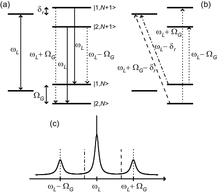
Figure 3: Sketch of the energy levels of the dressed-atom. a) Spontaneous emission lines leading to the Mollow triplet. b) Absorption lines. c) Overlap of the fluorescence spectrum (solid line) with the absorption lines of the 2-level system (dotted lines) and with those due to the third level (dashed lines).

(i) $\Omega,\left|\Delta\right|\gg\Gamma$. In general, for large detunings and intensities and large light-shifts ($\delta_{r}=\frac{1}{2}\left(\sqrt{\Delta^{2}+\Omega^{2}}-\left|\Delta\right|\right)\gg\Gamma$), the resonant term of the 2-level system dominates the sum, and all the other terms should be dropped to remain consistent with the secular approximation done before. The resulting re-absorption cross-section has thus the following simple expression:

$$\sigma_{R}=\frac{\sigma_{0}}{4}\,\frac{\Delta^{2}\Omega^{2}}{4\Delta^{4}+8\Delta^{2}\Omega^{2}+3\Omega^{4}}$$ (16)

This result is consistent, within a factor of 2, with the limit values given for $\Omega\gg\left|\Delta\right|\gg\Gamma$ and $\left|\Delta\right|\gg\Omega\gg\Gamma$ in the appendix of Ref. pruvost2000 .

(ii) $\left|\Delta\right|\gg\Omega$. The contribution due to the non-coupled level is never exactly resonant. However, in this case, the light-shift, $\delta_{r}\simeq\Omega^{2}/4\left|\Delta\right|$, can be arbitrarily small, leading to an almost resonant behaviour if $\delta_{r}\lesssim\Gamma$. In the case where $\left|\Delta\right|\gg\Omega\gg\Gamma$ and $\Gamma\gg\Omega^{2}/4\left|\Delta\right|$, we take into account the quasi resonant contribution of the third level:

$$\sigma_{R}=\frac{\sigma_{0}}{8}\,\frac{\Omega^{2}}{\Delta^{2}}$$ (17)

Note that (17) is not the limit of (16) when $\left|\Delta\right|\gg\Omega$, although it has the same form.

(iii) $\Omega\ll\Gamma$. When the intensity is very small, the resonant or quasi-resonant contributions go to zero and the leading term corresponds to the reabsorption of the elastic component:

$$\sigma_{R}=\frac{\sigma_{0}}{4}\,\frac{\Gamma^{2}}{\Delta^{2}}$$ (18)

(iv) $\left|\Delta\right|\ll\Gamma$. For small detunings, the reabsorption by a 2-level atom goes to zero because the transition is strongly saturated. Then, the contribution of the third level, although it is non-resonant, has to be taken into account. We have:

$$\sigma_{R}=\sigma_{0}\frac{25}{48}\,\frac{\Gamma^{2}}{\Omega^{2}}$$ (19)

The above results allow us to write in the different regimes the contribution of the multiple scattering to the MOT dynamics. These expressions are rather simple as compared to those found in the literature. It is interesting to note that $\sigma_{R}$ is always larger than the absorption cross-section for the trapping beams. This is very often assumed in previous papers, as stated in sesko1991 . We have demonstrated here that, in the secular regime for three level atoms, it is always true. The above expressions of $\sigma_{R}$, together with the expression of the trapping force derived in the previous paragraph, allow us to write a full model of the MOT, which can be used as a basis for future analyses.

7 Conclusion

In this paper, we built a model for a 1D Magneto-Optical Trap as general as possible. We show that such a trap is described by a Vlasov-Fokker-Planck equation with a second relaxation term and a source term, both originating in the bath of hot atoms of the atomic vapor. This VFP equation is coupled to a set of two differential equations describing the beam propagation in the cold atoms. This system could be considered as relatively similar to plasmas, where the role of the thermal bath is played by the trapping beams. However, it appears that the MOT differs from plasmas on two important points: the second thermal bath, formed by the hot atoms, induces new interactions as compared to plasmas; the trapping beams are not a “thermal” bath, as the atoms act on them through the absorption.

In the last section of this paper, we derive in a more detailed way the equations established in the previous sections, and compare the results with those found in the litterature. We show that important correction terms must be taken into account in the evaluation of the trapping forces, and we establish the expression of the multiple scattering in different situations.

These equations aimed to be a basis for future developments. They should contribute to obtain a better agreement between the experimental observations and the theoretical predictions. Let us remember that the previous existing models were only in qualitative agreement with the experimental observations, in particular for the situations out of equilibrium. Using this model to study the instabilities in the cold atoms should give a better insight of the mechanism in which they originate. Thus a natural continuation of the present work would be to extend this model to the 3D traps.

8 Appendix

In this appendix, we present the detailed calculations of the re-absorption cross section, resulting from the overlap of the fluorescence spectrum of an atom somewhere in the sample with the absorption spectrum of another atom elsewhere. In the $J=0\rightarrow J^{\prime}=1$ transition considered here, we have three sublevels in the excited state, and the polarization of the scattered photon will not match exactly the polarization of the local field. For the sake of simplicity, let us consider here the case where the trapping beams have the same intensity. In real experiments, it cannot be true everywhere in the sample because of the shadow effect, but the deviation remains on the order of 10%. In this simple case, the resulting polarization of the total trapping field is everywhere linear, but its direction follows an helix. The laser wavelength is the scale for changing the relative phase between $\Omega_{+}$ and $\Omega_{-}$, because the two beams are contrapropagating. As soon as we are not interested in what happens at length scales smaller than the laser wavelength, we can estimate that one half of the photons in the bath will interact with the transition between the ground state and the coupled one, while the other half of them can excite the atom to the non-coupled level. The total re-absorption cross-section, $\sigma_{R}$, is thus the average of the usual cross-section, $\sigma_{R}^{(2)}$, calculated with a 2-level atom pruvost2000 and of a new contribution, $\sigma_{R}^{(3)}$, coming from the presence of an excited level which is not coupled to the trapping field. The empty non-coupled state allows a strong absorption of the scattered light, while the absorption by the coupled state can be saturated by the trapping field.

As usual, when one works with the dressed atom model, the calculations are much simpler in the secular approximation. This approximation is valid as soon as the energy splitting is larger than the typical width of the levels, which is expressed by the condition:

$$\sqrt{\Delta^{2}+\Omega^{2}}\gg\Gamma$$ (20)

Please note that this relation does not require that both the detuning and the intensity are large, and some interesting limits can be examined with either $\Omega\lesssim\Gamma$ or $\left|\Delta\right|\lesssim\Gamma$, in the secular limit. First, we calculate the emission spectral density, $S\left(\omega\right)$, for an atom illuminated with the two trapping beams. Then, we evaluate the absorption spectra of another atom, also interacting with the trapping field. Two contributions appear in the absorption process: on one hand, the coupled excited level can still absorb light, leading to a contribution which is the one of a 2-level atom, $\sigma_{A}^{(2)}\left(\omega\right)$, and on the other hand, the non-coupled level has to contribute with $\sigma_{A}^{(3)}\left(\omega\right)$. Finally, we evaluate the total re-absorption cross-section, $\sigma_{R}$, with:

$$\sigma_{R} = \frac{1}{2}\left(\sigma_{R}^{(2)}+\sigma_{R}^{(3)}\right)$$ (21)

$$\sigma_{R}^{(2)} = \int\,\sigma_{A}^{(2)}\left(\omega\right)\,S\left(\omega\right)\,d\omega$$

$$\sigma_{R}^{(3)} = \int\,\sigma_{A}^{(3)}\left(\omega\right)\,S\left(\omega\right)\,d\omega$$

All these calculations are done using the formalism of the dressed atom, in the secular limit (20). The normalized fluorescence spectrum is given by:

$$S\left(\omega\right) = \frac{\left(c^{2}-s^{2}\right)^{2}}{c^{4}+s^{4}}\delta\left(\omega-\omega_{L}\right)+\frac{\left(2c^{2}s^{2}\right)^{2}}{c^{4}+s^{4}}L\left(\omega-\omega_{L},\Gamma_{p}\right)$$

$$+c^{2}s^{2}L\left(\omega-\omega_{L}-\Omega_{G},\Gamma_{c}\right)$$

$$+c^{2}s^{2}L\left(\omega-\omega_{L}+\Omega_{G},\Gamma_{c}\right)$$

where $\Omega_{G}=\sqrt{\Delta^{2}+\Omega^{2}}$ is the generalized Rabi frequency. The transformation from the bare basis to the dressed one is given by $c=cos\left(\theta\right)$, $s=sin\left(\theta\right)$, with the angle $\theta$ defined by $tg\left(2\theta\right)=-\frac{\Omega}{\Delta}$. $\delta\left(\omega-\omega_{L}\right)$ is the Dirac delta function, and $L\left(\omega,\Gamma\right)$ is the normalized Lorentzian:

$$L\left(\omega,\Gamma\right)=\frac{1}{\pi}\,\frac{\Gamma}{\omega^{2}+\Gamma^{2}}$$

and the relaxation rates for the populations and the coherences are:

$$\Gamma_{p} = \Gamma\left(1-2c^{2}s^{2}\right)$$ (22)

$$\Gamma_{c} = \frac{\Gamma}{2}\left(1+2c^{2}s^{2}\right)$$ (23)

The first term in $S\left(\omega\right)$ corresponds to the elastic scattering, while the three other terms are inelastic components. The last two terms are the sidebands of the Mollow triplet, centered in $\omega_{L}\pm\Omega_{G}$, which are proportional to the intensity when $\left|\Delta\right|\gg\Omega$.

The absorption spectra are given by:

$$\sigma_{A}^{(2)}\left(\omega\right) = \sigma_{0}\frac{\pi\Gamma}{2}\frac{c^{2}-s^{2}}{c^{4}+s^{4}}c^{4}L\left(\omega-\omega_{L}-\Omega_{G},\Gamma_{c}\right)$$

$$-\sigma_{0}\frac{\pi\Gamma}{2}\frac{c^{2}-s^{2}}{c^{4}+s^{4}}s^{4}L\left(\omega-\omega_{L}+\Omega_{G},\Gamma_{c}\right)$$

$$\sigma_{A}^{(3)}\left(\omega\right) = \sigma_{0}\frac{\pi\Gamma}{2}c^{6}L\left(\omega-\omega_{L}-\Omega_{G}+\delta_{r},\Gamma_{2}\right)$$

$$+\sigma_{0}\frac{\pi\Gamma}{2}s^{6}L\left(\omega-\omega_{L}+\delta_{r},\Gamma_{1}\right)$$

where $\delta_{r}$ is the light-shift, and $\Gamma_{1,2}$ are the relaxation rates for the coherences between the non-coupled level and the dressed states.

$$\delta_{r} = \frac{1}{2}\left(\Delta+\sqrt{\Delta^{2}+\Omega^{2}}\right)$$ (24)

$$\Gamma_{1} = \frac{\Gamma}{2}\left(1+c^{2}\right)$$ (25)

$$\Gamma_{2} = \frac{\Gamma}{2}\left(1+s^{2}\right)$$ (26)

The absorption spectrum of the 2-level part consists in two lines centred in $\omega_{L}\pm\Omega_{G}$, which means that they are resonantly excited by the two sidebands of the Mollow triplet. The two absorption lines due to the third level are centred in $\omega_{L}+\Omega_{G}-\delta_{r}$ and in $\omega_{L}-\delta_{r}$, then the excitation by the fluorescence light is not resonant if $\delta_{r}\gg\Gamma$. Because of the secular approximation we made for the calculation, it is incorrect to write $\sigma_{R}$ as the sum of 16 terms, coming from the overlap of the four components of the fluorescence with the four absorption lines. We have to consider separately the different cases.

In general, for large detunings and intensities ($\Omega,\left|\Delta\right|\gg\Gamma$) and large light-shifts ($\delta_{r}\gg\Gamma$), the resonant term of the 2-level system dominates the sum, and one should drop all the other terms to be consistent with the secular approximation done before. The resulting cross-section has thus the following simple expression:

$$\sigma_{R}=\frac{\sigma_{0}}{4}\,\frac{\Delta^{2}\Omega^{2}}{4\Delta^{4}+8\Delta^{2}\Omega^{2}+3\Omega^{4}}$$ (27)

As already mentioned, the contribution due to the non-coupled level is never exactly resonant. However, if $\left|\Delta\right|\gg\Omega$, the light-shift, $\delta_{r}\simeq\Omega^{2}/4\left|\Delta\right|$, can be arbitrarily small, leading to an almost resonant behaviour if $\delta_{r}\lesssim\Gamma$. In the case where $\left|\Delta\right|\gg\Omega\gg\Gamma$ and $\Gamma\gtrsim\Omega^{2}/4\left|\Delta\right|$, we take into account the quasi resonant contribution of the third level:

$$\sigma_{R}=\frac{\sigma_{0}\,\Omega^{2}}{16\,\Delta^{2}}\,\left\{1+\frac{16\,\Delta^{2}\,\Gamma^{2}}{\Omega^{4}+16\,\Delta^{2}\,\Gamma^{2}}\right\}$$ (28)

- (1) L. Guidoni and P. Verkerk, J. Opt. B: Quantum Semiclass. Opt. 1 R23 (1999)
- (2) Cold Molecules: Theory, Experiment, Applications, edited by Roman Krems, Bretislav Friedrich and William C Stwalley (CRC Press, Boca Raton, 2009)
- (3) M. H. Anderson, J. R. Ensher, M. R. Matthews, C. E. Wieman and E. A. Cornell, Science 269 198-201 (1995)
- (4) D. Wilkowski, J. Ringot, D. Hennequin and J. C. Garreau, Phys. Rev. Lett. 85 1839-1842 (2000)
- (5) G. Labeyrie, F. Michaud and R. Kaiser, Phys. Rev. Lett. 96, 023003 (2006)
- (6) D. Hennequin, Eur. Phys. J. D 28 135-147 (2004)
- (7) A. di Stefano, M. Fauquembergue, P. Verkerk and D. Hennequin, Phys. Rev. A 67 033404 (2003)
- (8) A. di Stefano, P. Verkerk and D. Hennequin, Eur. Phys. J. D 30 243-258 (2004)
- (9) T. Pohl, G. Labeyrie, and R. Kaiser, Phys. Rev. A 74, 023409 (2006)
- (10) T.G. Walker, D.W. Sesko, and C. Wieman, Phys. Rev. Lett. 64, 408 (1990)
- (11) L. Pruvost, I. Serre, H. T. Duong, and J. Jortner, Phys. Rev. A 61, 053408 (2000)
- (12) J. T. Mendonça, R. Kaiser, H. Terças, and J. Loureiro, Phys. Rev. A 78, 013408 (2008)
- (13) D.W. Sesko, T.G. Walker, and C. Wieman, J. Opt. Soc. Am. B 8 946 (1991)
- (14) H. Neunzert, M. Pulvirenti and L. Triolo, Math. Methods Appl. Sci. 6 527-538 (1984)
- (15) Javier Ramos-Caro and Guillermo A González, Class. Quantum Grav. 25 045011 (2008)
- (16) Dario Benedetto, Emanuele Caglioti, François Golse, and Mario Pulvirenti, Comm. Math. Sci. 2, 121 (2004)
- (17) R. Warnock, Nucl. Instrum. Methods Phys. Res., Sect. A 561, 186 (2006).
- (18) J. Dalibard and C. Cohen-Tannoudji, J. Opt. Soc. Am. B 6, 2023 (1989)
- (19) C. Cohen-Tannoudji, J. Dupont-Roc, and G. Grynberg, Atom-Photon Interactions (Wiley, New York, 2004)
- (20) B.R. Mollow, Phys. Rev. 188, 1969 (1969)