Electromagnetic production of kaon near threshold

Abstract

Kaon photo- and electroproduction off a proton near the production threshold are investigated by utilizing an isobar model. The background amplitude of the model is constructed from Feynman diagrams, whereas the resonance term is calculated by using the multipole formalism. It is found that both pseudoscalar and pseudovector models can nicely describe the available photoproduction data up to $W=50$ MeV above the threshold. The $\Lambda$ resonance $S_{01}(1800)$ is found to play an important role in improving the model. In the case of double polarization observables $O_{x}$ and $O_{z}$ our result corroborates the finding of Sandorfi et al. Due to the large contributions of the $K^{*}$ and $K_{1}$ vector mesons, extending the model to the case of electroproduction is almost impossible unless either special form factors that strongly suppress their contributions are introduced or all hadronic coupling constants are refitted to both photo- and electroproduction databases, simultaneously. It is also concluded that investigation of the kaon electromagnetic form factor is not recommended near the threshold region.

I Introduction

It has been known that a comprehensive phenomenological analysis of kaon photoproduction is still far away from what we expected one or two decades ago, in spite of the fact that there are ample experimental data with good quality recently provided by modern accelerators such as JLab in Newport News, ELSA in Bonn, and SPRING8 in Osaka. The reason for this set back is because of the high threshold energy, which not only “switches on” the strangeness degree of freedom, but also increases the level of complexity of phenomenological or theoretical models that attempt to describe the process. Already close to the production threshold ($W_{\rm thr.}=1609$ MeV for $K^{+}\Lambda$ photoproduction), a number of established nucleon resonances contribute to the process, for instance the $S_{11}(1650)$, $D_{15}(1675)$, and $F_{15}(1680)$. Even below the threshold there are the well known Roper resonance $P_{11}(1440)$ along with two other four-star resonances $D_{13}(1520)$ and $S_{11}(1535)$. Furthermore, the presence of strangeness degree of freedom insists on the use of SU(3) symmetry in the reaction mechanism, rather than SU(2) as in the case of pion production, which clearly makes the theoretical formalism more difficult.

In the last decades tremendous efforts have been devoted to model kaon photoproduction process. Most of them have been performed in the framework of tree-level isobar models abw ; Adelseck:1990ch ; williams ; Han:1999ck ; kaon-maid ; Janssen:2001wk ; delaPuente:2008bw , coupled channel approaches Feuster:1998cj ; Chiang:2001pw ; Shklyar:2005xg ; Julia-Diaz:2006is ; Anisovich:2007bq , Regge model Guidal:1997hy , or quark models Li:1995sia ; Lu:1995bk . Extending the energy range of isobar models to higher region by utilizing Regge formalism has also been pursued recently Mart:2003yb ; Mart:2004au ; Corthals:2005ce ; Vancraeyveld:2009qt . At present, experimental data are abundant from threshold up to 2.5 GeV. In this energy range there are 19 nucleon resonances in the Particle Data Book Amsler:2009 table (PDG), which may propagate in the $s$-channel intermediate states. In addition, there are hyperon and meson resonances that may also influence the background terms of the process. To take into account all these excited states is naturally a daunting task, since their hadronic and electromagnetic coupling constants are mostly unknown. There is a possibility to fit all these unknown parameters, however, the accuracies of presently available data still allow for too many possible solutions. Furthermore, the extracted couplings are quite often “nonphysical”, in the sense that their values are much smaller or much larger than the widely known pion coupling constant $g_{\pi NN}$. In the literature, a number of recipes have been put forward to avoid this problem, e.g., by limiting the number of resonances, by taking into account as many as possible constraints that are relevant to the process, or by combining these two methods.

Except limiting the energy of interest, there is no firm argument for limiting the number of resonances that should be put into the model. In the previous works, the goal to construct a very simple elementary operator for use in nuclear physics was sometimes used for this purpose abw ; williams ; kaon-maid . The argument of duality is also proposed to this end saghai96 . As a result, the number of phenomenological models describing kaon photoproduction was quickly increasing in the last decades. These models differ chiefly by the number and type of resonances used as well as, quite obviously, the values of extracted coupling constants.

The exact values of coupling constants are a long-standing problem. Even for the main coupling constants $g_{K\Lambda N}$ and $g_{K\Sigma N}$ there is so far no consensus as to which values should be used in the electromagnetic production of kaon. The SU(3) symmetry dictates the values of $g_{K\Lambda N}/\sqrt{4\pi}=-4.4{\rm~{}to~{}}-3.0$ and $g_{K\Sigma N}/\sqrt{4\pi}=+0.9{\rm~{}to~{}}+1.3$, given that the SU(3) is broken at the level of 20% Adelseck:1990ch . These values are consistent with those extracted from the $K$-$N$ or $Y$-$N$ scattering data anto ; boz . However, the QCD sum rules predicted significantly smaller values, i.e. $g_{K\Lambda N}/\sqrt{4\pi}=-1.96$ and $g_{K\Sigma N}/\sqrt{4\pi}=+0.33$ choe . On the other hand, the values extracted from kaon photoproduction are mostly much smaller than the SU(3) prediction, unless hadronic form factors were used in hadronic vertices or some absorptive factors are applied to reduce the Born terms tkb . These facts indicate that the problem of the $g_{K\Lambda N}$ and $g_{K\Sigma N}$ values is far from settled at present. Other coupling constants, such as those of $K^{*}$ and $K_{1}$ intermediate states can be also estimated with the help of SU(3) symmetry and a number of parameters extracted from other reactions. Their values are by all means less accurate than the values of $g_{K\Lambda N}$ and $g_{K\Sigma N}$.

A quick glance to the $K^{+}\Lambda$ photoproduction data base will reveal that there are more than 100 data points of differential cross section for the energy range from threshold up to 50 MeV above the threshold, available from the SAPHIR Glander:2003jw and CLAS Bradford:2005pt collaborations. This indicates that a phenomenological analysis of kaon photoproduction near the production threshold is already possible. To the best of our knowledge, there was no such an analysis performed with these data. The latest study of kaon photoproduction from threshold up to 14 MeV above the $E_{\gamma,{\rm thr}}^{\rm lab}$ was performed by Cheoun et al. Cheoun:1996kn more than a decade ago. Since there were no data available at that time, Cheoun et al. predicted the total cross section of the $\gamma+p\to{K^{+}}+\Lambda$ process by varying the value of $g_{K\Lambda N}/\sqrt{4\pi}$ from 0 to 4 and studied the difference between the pseudoscalar (PS) and pseudovector (PV) couplings in this reaction. They argued that measurement of the total cross section can determine the real value of this coupling constant. We note that for the SU(3) value of the $g_{K\Lambda N}/\sqrt{4\pi}$, the total cross sections for both PS and PV couplings at 10 MeV above $E_{\gamma,{\rm thr}}^{\rm lab}$ are predicted to be around 5 $\mu$b, whereas for the value accepted by the QCD sum rule the cross sections would be slightly more than 1 $\mu$b. It is interesting to compare these predictions with the currently available data (see Fig. 3 in Section V) and find that none of these predictions is right, since at this energy the experimental cross section is found to be less than 0.4 $\mu$b.

From the facts presented above it is clear that investigation of kaon photoproduction near the production threshold is very important, because it could provide very important information on the simplest form of the reaction mechanism as well as information on the background terms. In the isobar model this also means information on the $t$- and $u$-channel intermediate states that contribute to the background terms. Such information is obviously very difficult to obtain at high energies due to the complicated structure of reaction amplitude at this stage. Furthermore, since models that describe the production at threshold are in general quite simple, the individual contributions of intermediate states to this process can be easily studied. In summary, the result of this investigation should become a stepping stone for the construction of extended models describing the photo- and electroproduction reaction at higher energies.

In this paper we present our analysis on the $\gamma+p\to{K^{+}}+\Lambda$ process near the production threshold, i.e. up to 50 MeV above the $W_{\rm thr.}$, as well its extension to the electroproduction case $e+p\to e+K^{+}+\Lambda$. We note that a new version of kaon photoproduction data from CLAS collaboration has been published recently McCracken:2009ra . However, since the behavior of these data at the threshold region is similar to that shown by the previous ones Bradford:2005pt , we believe that it is sufficient to use the previous version of CLAS data Bradford:2005pt for the photoproduction process in the following discussion for the sake of simplicity. As a starting point we consider the resonances suggested by Cheoun et al. Cheoun:1996kn (see Table II of Ref. Cheoun:1996kn ) for the possible resonance intermediate states in the energy range of interest. However, different from the work of Cheoun et al., to simplify the fitting process in this work we fix the values of the $g_{K\Lambda N}$ and $g_{K\Sigma N}$ to the SU(3) symmetry prediction, as in the case of Kaon-Maid kaon-maid , though we do not use the hadronic form factors in all hadronic vertices. For the resonance formalism, we use the Breit-Wigner multipole form as suggested by Drechsel et al. hanstein99 and Tiator et al. Tiator:2003uu . The advantage of using this formalism as compared to the covariant one is that it provides a direct comparison of the extracted helicity photon couplings with the PDG values. Moreover, the multipole formalism does not produce unnecessary additional background terms that will interfere with the pure ones, as in the case of the covariant calculation. To further reduce the number of free parameters in our model we also fix the resonance parameters to the PDG values.

This paper is organized as follows. In Section II we present the formalism of our model in the PS theory. Section III briefly discusses resonance formalism of our model. In Section IV we present the difference between PS and PV amplitudes. The numerical results and comparison between experimental data for kaon photoproduction and model calculations will be given in Section V. In Section VI we discuss the extension of our model to the case of electroproduction and the effect of the available kaon electroproduction data on the result of our previous fit. In Section VII we summarize our findings.

II Pseudoscalar coupling

Let us consider photo- and electroproduction process that can be represented as a real and virtual photon production

$$\gamma_{\rm r,v}(k)+p(p_{p})\to K^{+}(q_{K})+\Lambda(p_{\Lambda})~{}.$$ (1)

As discussed in the previous section, the background terms of this process are obtained from a series of tree-level Feynman diagrams shown in Fig. 1. They consist of the standard $s$-, $u$-, and $t$-channel Born terms along with the $K^{*+}(892)$ and $K_{1}(1270)$ $t$-channel vector meson. The energy near threshold can be considered as low energy, therefore, we would expect that no hadronic form factors is required in all hadronic vertices of the diagrams in Fig. 1. This has an obvious advantage, i.e., we can further limit the number of free parameters as well as uncertainties in our model. In Ref. Bydzovsky:2006wy it is shown that the use of hadronic form factor could lead to an underprediction of differential cross section data at forward angles.

Using the standard procedure in the pseudoscalar theory the transition amplitude for kaon photo- and electroproduction off a proton reads

$${\cal M}^{\rm ps} = {\bar{u}}_{\Lambda}(\mbox{\boldmath${p}$}_{\Lambda})\biggl{[}ig_{K\Lambda N}\gamma_{5}\Bigl{\{}\frac{p\!\!\!/_{p}+k\!\!\!/+m_{p}}{s-m_{p}^{2}}\Bigl{(}\epsilon\!\!/eF_{1}^{p}+i\sigma^{\mu\nu}\epsilon_{\mu}k_{\nu}\mu_{p}F_{2}^{p}\Bigr{)}-\frac{k\cdot\epsilon}{k^{2}}eF_{1}^{p}\Bigr{\}}$$ (2)

$$+i\sigma^{\mu\nu}\epsilon_{\mu}k_{\nu}\mu_{\Lambda}F_{2}^{\Lambda}\frac{p\!\!\!/_{\Lambda}-k\!\!\!/+m_{\Lambda}}{u-m_{\Lambda}^{2}}ig_{K\Lambda N}\gamma_{5}+ig_{K\Lambda N}\gamma_{5}\Bigl{\{}\frac{(2q_{K}-k)\cdot\epsilon}{t-m_{K}^{2}}+\frac{k\cdot\epsilon}{k^{2}}\Bigr{\}}eF^{K}$$

$$+\frac{i}{M(t-m_{K^{*}}^{2}+im_{K^{*}}\Gamma_{K^{*}})}\Bigl{\{}g^{V}_{K^{*}\Lambda N}\gamma_{\mu}-\frac{g^{T}_{K^{*}\Lambda N}}{m_{p}+m_{\Lambda}}i\sigma^{\mu\nu}(q_{K}-k)_{\nu}\Bigr{\}}$$

$$\times i\varepsilon_{\mu\nu\rho\sigma}\epsilon^{\nu}k^{\rho}q_{K}^{\sigma}\,g_{K^{*}K\gamma}F^{K^{*}}$$

$$+\frac{1}{M(t-m_{K_{1}}^{2}+im_{K_{1}}\Gamma_{K_{1}})}\Bigl{\{}g^{V}_{K_{1}\Lambda N}\gamma^{\mu}\gamma_{5}+\frac{g^{T}_{K_{1}\Lambda N}}{m_{p}+m_{\Lambda}}(p\!\!\!/_{\Lambda}-p\!\!\!/_{p})\gamma^{\mu}\gamma_{5}\Bigr{\}}$$

$$\times\left\{(q_{K}-k)\cdot\epsilon\,k_{\mu}-(q_{K}-k)\cdot k\,\epsilon_{\mu}\right\}\,g_{K_{1}K\gamma}F^{K_{1}}$$

$$+i\sigma^{\mu\nu}\epsilon_{\mu}k_{\nu}\mu_{T}F_{2}^{T}\frac{p\!\!\!/_{\Sigma}-k\!\!\!/+m_{\Sigma}}{u-m_{\Sigma}^{2}}ig_{K\Sigma N}\gamma_{5}$$

$$+i\sigma^{\mu\nu}\epsilon_{\mu}k_{\nu}\mu_{Y^{*}}F_{2}^{Y^{*}}\frac{p\!\!\!/_{Y^{*}}-k\!\!\!/+m_{Y^{*}}}{u-m_{Y^{*}}^{2}+im_{Y^{*}}\Gamma_{Y^{*}}}ig_{KY^{*}N}\gamma_{5}\,\biggr{]}\,u_{p}({\mbox{\boldmath${p}$}}_{p})~{},$$

where $\mu_{p}$ and $\mu_{\Lambda}$ denote the magnetic moments of the proton and $\Lambda$-hyperon, respectively, $\epsilon$ is the photon polarization vector, $F^{i}$ are the electromagnetic form factors of the $i$ intermediate states that will be discussed in Section VI, and $M=1$ GeV is introduced to make the coupling constants of $K^{*}$ and $K_{1}$ dimensionless.

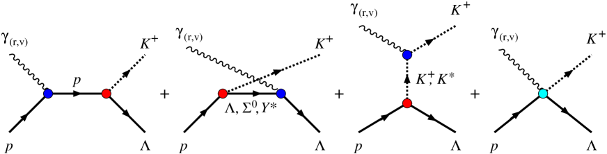
Figure 1: (Color online) Feynman diagrams of the background amplitude. Note that the last diagram (contact or seagull diagram) is used to maintain gauge invariance in the pseudovector theory.

The transition amplitude in Eq. (2) can be written as deo

$$M_{\rm fi} = \bar{u}(\mbox{\boldmath${p}$}_{\Lambda})\sum_{j=1}^{6}A_{j}(s,t,k^{2})M_{j}u(\mbox{\boldmath${p}$}_{p})~{},$$ (3)

where $s$ and $t$ are the usual Mandelstam variables, defined by

$$s=(k+p_{p})^{2},~{}~{}t=(k-q_{K})^{2},~{}~{}u~{}=~{}(k-p_{\Lambda})^{2}~{},$$ (4)

whereas the gauge and Lorentz invariant matrices $M_{j}$ are given by

$$M_{1} = {\textstyle\frac{1}{2}}\gamma_{5}\left(\epsilon\!\!/k\!\!\!/-k\!\!\!/\epsilon\!\!/\right)~{},$$ (5a)

$$M_{2} = \gamma_{5}\left[(2q_{K}-k)\cdot\epsilon P\cdot k-(2q_{K}-k)\cdot kP\cdot\epsilon\right]~{},$$ (5b)

$$M_{3} = \gamma_{5}\left(q_{K}\cdot k\epsilon\!\!/-q_{K}\cdot\epsilon k\!\!\!/\right)~{},$$ (5c)

$$M_{4} = i\epsilon_{\mu\nu\rho\sigma}\gamma^{\mu}q_{K}^{\nu}\epsilon^{\rho}k^{\sigma}~{},$$ (5d)

$$M_{5} = \gamma_{5}\left(q_{K}\cdot\epsilon k^{2}-q_{K}\cdot kk\cdot\epsilon\right)~{},$$ (5e)

$$M_{6} = \gamma_{5}\left(k\cdot\epsilon k\!\!\!/-k^{2}\epsilon\!\!/\right)~{},$$ (5f)

where $P=\frac{1}{2}(p_{p}+p_{\Lambda})$, and $\epsilon_{\mu\nu\rho\sigma}$ is the four dimensional Levi-Civita tensor with $\epsilon_{0123}=+1$. We note that the definition of the invariant matrices above is slightly different from those given in Refs. denn ; pasquini , specifically the $M_{4}$ amplitude. The functions $A_{i}$ therefore read

$$A_{1}^{\rm PS} = -\frac{eg_{K\Lambda N}}{s-m_{p}^{2}}\Bigl{(}F_{1}^{p}+\kappa_{p}\frac{m_{p}-m_{\Lambda}}{2m_{p}}F_{2}^{p}\Bigr{)}-\frac{eg_{K\Lambda N}}{u-m_{\Lambda}^{2}}\frac{m_{\Lambda}-m_{p}}{2m_{\Lambda}}\kappa_{\Lambda}F_{2}^{\Lambda}$$ (6a)

$$-\frac{eG_{K\Sigma N}}{u-m_{\Sigma}^{2}}\frac{m_{\Sigma}-m_{p}}{m_{\Sigma}+m_{\Lambda}}F_{2}^{T}-\frac{G^{T}_{K^{*}}tF^{K^{*}}}{M(t-m_{K^{*}}^{2}+im_{K^{*}}\Gamma_{K^{*}})(m_{p}+m_{\Lambda})}$$

$$+\frac{eG_{Y^{*}}F_{2}^{Y^{*}}}{u-m_{Y^{*}}^{2}+im_{Y^{*}}\Gamma_{Y^{*}}}\left\{-\frac{m_{p}+m_{Y^{*}}}{m_{\Lambda}+m_{Y^{*}}}+\frac{i\Gamma_{Y^{*}}}{2(m_{\Lambda}+m_{Y^{*}})}\right\}~{},$$

$$A_{2}^{\rm PS} = \frac{eg_{K\Lambda N}}{s-m_{p}^{2}}\frac{2F_{1}^{p}}{t-m_{K}^{2}}+\frac{G^{T}_{K^{*}}F^{K^{*}}}{M(t-m_{K^{*}}^{2}+im_{K^{*}}\Gamma_{K^{*}})(m_{p}+m_{\Lambda})}\left(1+\frac{k^{2}}{t-m_{K}^{2}}\right)$$ (6b)

$$-\frac{G^{T}_{K_{1}}F^{K_{1}}}{M(t-m_{K_{1}}^{2}+im_{K_{1}}\Gamma_{K_{1}})(m_{p}+m_{\Lambda})}\left(1+\frac{k^{2}}{t-m_{K}^{2}}\right)~{},$$

$$A_{3}^{\rm PS} = \frac{eg_{K\Lambda N}}{s-m_{p}^{2}}\frac{\kappa_{p}F_{2}^{p}}{2m_{p}}-\frac{eg_{K\Lambda N}}{u-m_{\Lambda}^{2}}\frac{\kappa_{\Lambda}F_{2}^{\Lambda}}{2m_{\Lambda}}-\frac{eG_{K\Sigma N}}{u-m_{\Sigma}^{2}}\frac{F_{2}^{T}}{m_{\Sigma}+m_{\Lambda}}$$ (6c)

$$-\frac{G^{T}_{K^{*}}F^{K^{*}}}{M(t-m_{K^{*}}^{2}+im_{K^{*}}\Gamma_{K^{*}})}\frac{m_{\Lambda}-m_{p}}{m_{\Lambda}+m_{p}}$$

$$+\frac{(m_{\Lambda}+m_{p})G^{V}_{K_{1}}+(m_{\Lambda}-m_{p})G^{T}_{K_{1}}}{M(t-m_{K_{1}}^{2}+im_{K_{1}}\Gamma_{K_{1}})}\frac{F^{K_{1}}}{m_{\Lambda}+m_{p}}$$

$$+\frac{eG_{Y^{*}}F_{2}^{Y^{*}}}{u-m_{Y^{*}}^{2}+im_{Y^{*}}\Gamma_{Y^{*}}}\frac{1}{m_{\Lambda}+m_{Y^{*}}}~{},$$

$$A_{4}^{\rm PS} = \frac{eg_{K\Lambda N}}{s-m_{p}^{2}}\frac{\kappa_{p}F_{2}^{p}}{2m_{p}}+\frac{eg_{K\Lambda N}}{u-m_{\Lambda}^{2}}\frac{\kappa_{\Lambda}F_{2}^{\Lambda}}{2m_{\Lambda}}+\frac{eG_{K\Sigma N}}{u-m_{\Sigma}^{2}}\frac{F_{2}^{T}}{m_{\Sigma}+m_{\Lambda}}$$ (6d)

$$+\frac{G^{V}_{K^{*}}F^{K^{*}}}{M(t-m_{K^{*}}^{2}+im_{K^{*}}\Gamma_{K^{*}})}-\frac{eG_{Y^{*}}F_{2}^{Y^{*}}}{u-m_{Y^{*}}^{2}+im_{Y^{*}}\Gamma_{Y^{*}}}\frac{1}{m_{\Lambda}+m_{Y^{*}}}~{},$$

$$A_{5}^{\rm PS} = \frac{eg_{K\Lambda N}}{t-m_{K}^{2}}\left\{\left(-\frac{2}{k^{2}}+\frac{1}{s-m_{p}^{2}}\right)F_{1}^{p}+\frac{2}{k^{2}}F^{K}\right\}$$ (6e)

$$-\frac{G^{T}_{K^{*}}F^{K^{*}}}{M(t-m_{K^{*}}^{2}+im_{K^{*}}\Gamma_{K^{*}})(m_{p}+m_{\Lambda})}\left\{\frac{(s-m_{p}^{2})-(u-m_{\Lambda}^{2})}{2(t-m_{K}^{2})}\right\}$$

$$+\frac{G^{T}_{K_{1}}F^{K_{1}}}{M(t-m_{K_{1}}^{2}+im_{K_{1}}\Gamma_{K_{1}})(m_{p}+m_{\Lambda})}\left\{\frac{(s-m_{p}^{2})-(u-m_{\Lambda}^{2})}{2(t-m_{K}^{2})}\right\}~{},$$

$$A_{6}^{\rm PS} = -\frac{G^{T}_{K^{*}}F^{K^{*}}}{M(t-m_{K^{*}}^{2}+im_{K^{*}}\Gamma_{K^{*}})}\frac{m_{\Lambda}-m_{p}}{m_{\Lambda}+m_{p}}$$ (6f)

$$+\frac{(m_{\Lambda}+m_{p})G^{V}_{K_{1}}+(m_{\Lambda}-m_{p})G^{T}_{K_{1}}}{M(t-m_{K_{1}}^{2}+im_{K_{1}}\Gamma_{K_{1}})}\frac{F^{K_{1}}}{m_{\Lambda}+m_{p}}~{},$$

where $\kappa_{p}$ and $\kappa_{\Lambda}$ denote the anomalous magnetic moments of the proton and $\Lambda$ hyperon; $G^{V}_{K^{*}}=g_{K^{*}K\gamma}g_{K^{*}YN}^{V}$, $G^{T}_{K^{*}}=g_{K^{*}K\gamma}g_{K^{*}YN}^{T}$, $G^{V}_{K_{1}}=g_{K_{1}K\gamma}g_{K_{1}YN}^{V}$, $G^{T}_{K_{1}}=g_{K_{1}K\gamma}g_{K_{1}YN}^{T}$, $G_{Y^{*}}=\kappa_{Y^{*}}g_{KY^{*}N}$, and $G_{K\Sigma N}=\kappa_{T}g_{K\Sigma N}$. Note that the gauge invariance ensures that $A_{5}$ is still finite at the photon point $k^{2}=0$. Thus, there is no singularity in Eq. (6e) in the limit of $k\to 0$ and the transition from electroproduction to photoproduction is still smooth.

III The Resonance Amplitude

Since experimental data used in this calculation is limited up to 50 MeV above the threshold, only the resonance state $S_{11}(1650)$ contributes to the process. As a consequence only the resonant electric multipole $E_{0+}$ amplitude exists and the resonance contribution is extremely simplified. Following the work of Drechsel et al. hanstein99 and Tiator et al. Tiator:2003uu (see also the discussion in Section II.B of Ref. Mart:2006dk ), we can write the resonant electric multipole in the Breit-Wigner form as

$$E_{0+}(W) = {\bar{E}}_{0+}\,c_{K\Lambda}\,\frac{f_{\gamma R}(W)\,\Gamma_{\rm tot}(W)m_{R}\,f_{KR}(W)}{m_{R}^{2}-W^{2}-im_{R}\Gamma_{\rm tot}(W)}~{}e^{i\phi}~{},$$ (7)

where $W$ represents the total c.m. energy, the isospin factor $c_{K\Lambda}=-1$ Mart:2006dk , $f_{KR}$ is the usual Breit-Wigner factor describing the decay of a resonance $R$ with a total width $\Gamma_{\rm tot}(W)$ and physical mass $m_{R}$. The $f_{\gamma R}$ indicates the $\gamma NR$ vertex and $\phi$ represents the phase angle. The Breit-Wigner factor $f_{KR}$ is given by

$$f_{KR}(W) = \left[\frac{1}{2\pi}\frac{k_{W}}{|\mbox{\boldmath${q}$}_{K}|}\frac{m_{p}}{W}\frac{\Gamma_{K\Lambda}}{\Gamma_{\rm tot}^{2}}\right]^{1/2}~{}~{},~{}~{}~{}~{}k_{W}~{}=~{}\frac{W^{2}-m_{p}^{2}}{2W}~{},$$ (8)

with $m_{p}$ the proton mass. The energy dependent partial width $\Gamma_{K\Lambda}$ is defined through

$$\Gamma_{K\Lambda} = \beta_{K}\Gamma_{R}\frac{|\mbox{\boldmath${q}$}_{K}|}{q_{R}}\,\frac{W_{R}}{W}~{},$$ (9)

where $\beta_{K}$ is the single kaon branching ratio, $\Gamma_{R}$ and $q_{R}$ are the total width and kaon c.m. momentum at $W=m_{R}$, respectively. The $\gamma NR$ vertex is parameterized through

$$f_{\gamma R} = \frac{k_{W}}{k_{R}}~{},$$ (10)

where $k_{R}$ is equal to $k_{W}$ calculated at $W=m_{R}$.

The total width appearing in Eqs. (7) and (8) is the sum of $\Gamma_{K}$ and the “inelastic” width $\Gamma_{\rm in}$. In this work we assume the dominance of the pion decay channel and we parameterize the width by using

$$\Gamma_{\rm tot}~{}=~{}\Gamma_{K\Lambda}+\Gamma_{\rm in}~{},~{}~{}~{}~{}\Gamma_{\rm in}~{}=~{}(1-\beta_{K})\Gamma_{R}\left(\frac{q_{\pi}}{q_{0}}\right)^{4}\left(\frac{X^{2}+q_{0}^{2}}{X^{2}+q_{\pi}^{2}}\right)^{2}~{},$$ (11)

with $q_{\pi}$ the momentum of the $\pi$ in the decay of $R\to\pi+N$ in c.m. system, $q_{0}=q_{\pi}$ calculated at $W=m_{R}$, and the damping parameter $X$ is assumed to be 500 MeV hanstein99 .

The electric multipole photon coupling ${\bar{E}}_{0+}$ in Eq. (7) is related to the helicity photon coupling $A_{1/2}^{0+}$ through ${\bar{E}}_{0+}=-A_{1/2}^{0+}$. The scalar multipole photon coupling ${\bar{S}}_{0+}$ has the same form as Eq. (7). It is related to the helicity photon coupling $S_{1/2}^{0+}$ through ${\bar{S}}_{0+}=-\sqrt{2}S_{1/2}^{0+}$. To calculate the cross section we combine the CGLN amplitudes from the background and resonance terms. The CGLN amplitudes $F_{1}$-$F_{6}$ germar for the background terms are calculated from the functions $A_{1}$-$A_{6}$ given in Eq. (6), in the case of PS coupling. Since we have only $S_{11}(1650)$ as the resonance, the CGLN amplitudes in the resonance part becomes quite simple, i.e.,

$$F_{1} = {\bar{E}}_{0+}~{},$$ (12a)

$$F_{5} = \frac{k_{0}}{|\mbox{\boldmath${k}$}|}{\bar{S}}_{0+}~{}.$$ (12b)

IV Pseudovector coupling

In the pseudovector theory we have to change the vertex $\gamma_{5}g_{K\Lambda N}$ to $\gamma_{5}q\!\!\!/_{K}g_{K\Lambda N}^{\rm PV}$, where $q_{K}$ is the momentum of the kaon leaving the vertex and the pseudovector coupling constant $g_{K\Lambda N}^{\rm PV}$ is related to the pseudoscalar one through $g_{K\Lambda N}^{\rm PV}=g_{K\Lambda N}/(m_{p}+m_{\Lambda})$ deo . To maintain gauge invariance, the so-called contact (seagull) term shown in Fig. 1 is added. Therefore, the functions $A_{i}$ in the pseudovector theory are related to those of the pseudoscalar theory given by Eq. (6) through

$$A_{1}^{\rm PV} = A_{1}^{\rm PS}-\lambda_{\rm PV}\left[\frac{eg_{K\Lambda N}}{m_{p}+m_{\Lambda}}\left(\frac{\kappa_{p}F_{2}^{p}}{2m_{p}}+\frac{\kappa_{\Lambda}F_{2}^{\Lambda}}{2m_{\Lambda}}\right)-\frac{eG_{K\Sigma N}}{m_{\Lambda}+m_{\Sigma}}~{}\frac{F_{2}^{T}}{m_{p}+m_{\Sigma}}\right.$$ (13a)

$$-\left.\frac{eG_{Y^{*}}F_{2}^{Y^{*}}}{u-m_{Y^{*}}^{2}+im_{Y^{*}}\Gamma_{Y^{*}}}~{}\frac{1}{m_{\Lambda}+m_{Y^{*}}}\biggl{\{}2m_{Y^{*}}+\frac{u-m_{Y^{*}}^{2}}{m_{Y^{*}}+m_{p}}-\frac{i\Gamma_{Y^{*}}}{2}\biggr{\}}\right],~{}~{}$$

$$A_{3}^{\rm PV} = A_{3}^{{\rm PS}}-\lambda_{\rm PV}\frac{eG_{Y^{*}}F_{2}^{Y^{*}}}{u-m_{Y^{*}}^{2}+im_{Y^{*}}\Gamma_{Y^{*}}}~{}\frac{1}{m_{p}+m_{Y^{*}}}\biggl{\{}\frac{2m_{Y^{*}}}{m_{\Lambda}+m_{Y^{*}}}-\frac{i\Gamma_{Y^{*}}}{2(m_{\Lambda}+m_{Y^{*}})}\biggr{\}},~{}~{}$$ (13b)

$$A_{4}^{\rm PV} = A_{4}^{{\rm PS}}+\lambda_{\rm PV}\frac{eG_{Y^{*}}F_{2}^{Y^{*}}}{u-m_{Y^{*}}^{2}+im_{Y^{*}}\Gamma_{Y^{*}}}~{}\frac{1}{m_{p}+m_{Y^{*}}}\biggl{\{}\frac{2m_{Y^{*}}}{m_{\Lambda}+m_{Y^{*}}}-\frac{i\Gamma_{Y^{*}}}{2(m_{\Lambda}+m_{Y^{*}})}\biggr{\}},~{}~{}$$ (13c)

$$A_{6}^{\rm PV} = A_{6}^{\rm PS}-\lambda_{\rm PV}\frac{eg_{K\Lambda N}}{m_{p}+m_{\Lambda}}\left(\frac{F_{1}^{p}}{k^{2}}-\frac{F^{c}}{k^{2}}\right),$$ (13d)

where $\lambda_{\rm PV}$ represents the PS-PV mixing parameter, i.e., $\lambda_{\rm PV}=1$ for the pure PV coupling, $\lambda_{\rm PV}=0$ for the pure PS coupling, and $0<\lambda_{\rm PV}<1$ for the model with a PS-PV mixed coupling. The impact of the contact term is obvious in Eq. (13d), since without this term the longitudinal function $A_{6}$ would become singular at the photon point $k^{2}=0$.

V Results for Photoproduction

The cross sections and polarization observables are calculated from the function $A_{i}$ described above by using the standard formulas given in Ref. germar . These calculated observables are fitted to experimental data by adjusting the unknown coupling constants using the CERN-MINUIT code.

Table 1: Properties of the particles Amsler:2009 that might contribute to this process. This list is based on the work reported in Ref. Cheoun:1996kn . The particles used in the present analysis are indicated by $\surd$ in the last column.

Short	Resonance	I	$J^{\pi}$	Mass	Width	Used in the
Notation	Notation			(MeV)	(MeV)	Present Work
$p$		$\frac{1}{2}$	$\frac{1}{2}^{+}$	$938.272$	-	$\surd$
$K^{+}$		$\frac{1}{2}$	$0^{-}$	$493.677$	-	$\surd$
$\Lambda$		0	$\frac{1}{2}^{+}$	$1115.683$	-	$\surd$
$\Sigma^{0}$		1	$\frac{1}{2}^{+}$	$1192.642$	-	$\surd$
$K^{*+}$	$K^{*+}(892)$	$\frac{1}{2}$	$1^{-}$	$891.66$	$50.8$	$\surd$
$K_{1}$	$K_{1}(1270)$	$\frac{1}{2}$	$1^{+}$	$1272$	$90$	$\surd$
$N^{*}_{1}$	$P_{11}(1440)$	$\frac{1}{2}$	$\frac{1}{2}^{+}$	$1440$	$300$	-
$N^{*}_{2}$	$S_{11}(1535)$	$\frac{1}{2}$	$\frac{1}{2}^{-}$	$1535$	$150$	-
$N^{*}_{3}$	$S_{11}(1650)$	$\frac{1}{2}$	$\frac{1}{2}^{-}$	$1655$	$165$	$\surd$
$Y^{*}_{1}$	$S_{01}(1405)$	0	$\frac{1}{2}^{-}$	$1406.5$	$50$	-
$Y^{*}_{2}$	$S_{01}(1670)$	0	$\frac{1}{2}^{-}$	$1670$	$35$	-
$Y^{*}_{3}$	$S_{01}(1800)$	0	$\frac{1}{2}^{-}$	$1800$	$300$	$\surd$
$Y^{*}_{4}$	$S_{11}(1750)$	1	$\frac{1}{2}^{-}$	$1750$	$90$	-

V.1 Numerical Results

The particles which might contribute to the kaon photoproduction near threshold have been listed in Ref. Cheoun:1996kn . In Table 1 we display this list and indicate the particle used in the present analysis. It is important to note that we do not include all those possible resonances because the inclusion of nucleon resonances below the production threshold is not possible in our resonance formalism (see Sec. III). Furthermore, from the observation of the $\chi^{2}$ obtained from the fits, we learn that the use of only one hyperon resonance, i.e. the $S_{01}(1800)$, in the background terms is found to be sufficient for reproducing the experimental data within their accuracies (see Subsection V.4). Adding more hyperon resonances does not significantly improve the $\chi^{2}$.

In the present analysis we maintain to use both $K^{*}(892)$ and $K_{1}(1270)$ meson resonances, since most of previous studies, e.g. Refs. Adelseck:1990ch ; Janssen:2001wk , found that they are necessary to reproduce the SU(3) values of main coupling constants in the fits. The values of main coupling constants are fixed to the SU(3) values, i.e. $g_{K\Lambda N}/\sqrt{4\pi}=-3.80$ and $g_{K\Sigma N}/\sqrt{4\pi}=1.20$, as in the case of Kaon-Maid kaon-maid . The coupling constants of $K^{*}$, $K_{1}$, and the hyperon resonance are fitted to the available experimental data. In principle, their values can be estimated from other sources with the help of SU(3) symmetry and other mechanisms. However, in our analysis, the existence of these intermediate states is very important to avoid the divergence of the calculated cross section. As has been briefly discussed in Introduction, in order to limit the number of free parameters, we fix the resonance parameters of $S_{11}(1650)$ to the PDG values given in Table 2. Thus, for the nucleon resonance, only the phase angle $\phi$ in Eq. (7) is extracted from experimental data.

Table 2: Properties of the $S_{11}(1650)$ resonance taken from the Review of Particle Properties Amsler:2009 .

Resonance	$M_{R}$	$\Gamma_{R}$	$\beta_{K}$	$A_{1/2}(p)$	Overall	Status
	(MeV)	(MeV)		($10^{-3}$ GeV-1/2)	status	seen in $K\Lambda$
$S_{11}(1650)$	$1655^{+15}_{-10}$	$165\pm 20$	$0.027\pm 0.004$	$+53\pm 16$	****	***

Obviously, there is no need to consider hadronic form factors here, since contribution from the background terms is still controllable. As shown by Refs. Adelseck:1990ch ; Hsiao:2000 , the background contribution starts to diverge at $W>1900$ MeV. At this stage, even combination of several nucleon and hyperon resonances is unable to damp the cross section. Thus, the use of hadronic form factors provides the only efficient mechanism to overcome this problem. Meanwhile, the problem of data inconsistency discussed e.g. in Refs. Mart:2006dk ; Bydzovsky:2006wy does not appear in the energy region of interest, since both CLAS and SAPHIR data agree each other up to 50 MeV above the threshold.

There are 139 experimental data points in our database for energies up to 50 MeV above $W_{\rm thr}$, consisting of 115 differential cross sections Glander:2003jw ; Bradford:2005pt , 18 recoil polarizations Glander:2003jw ; Bradford:2005pt ; lleres07 , and 6 photon beam asymmetries lleres07 . In addition, we have 18 data points of beam-recoil double polarizations, $O_{x}$ and $O_{z}$, and target asymmetry $T$ from the latest GRAAL measurement lleres09 .

A comparison between the extracted coupling constants in the present analysis and those obtained in previous works is given in Table 3. Our result corroborates the finding of previous studies, i.e. experimental data prefer the PS coupling. The $\chi^{2}$ of this model is clearly smaller than that of the PV one, which is an obvious consequence of the use the SU(3) main coupling constants. In the PV case, if we left these coupling constants to be determined by experimental data, we would then obtain smaller values like those found in previous studies Hsiao:2000 ; bennhold:1987 . The phenomenon originates from the fact that the standard PV Born terms yield a larger cross section compared to the standard PS Born terms. This problem can be alleviated by reducing the absolute values of the main coupling constants. In our case, since the coupling constants are fixed to the SU(3) values, the fit tried to reduce this through a destructive interference with other diagrams, e.g. by increasing the values of the hyperon resonance $Y_{3}^{*}$ coupling constant (see column 3 of Table 3). Nevertheless, this is insufficient to compete with the result of the PS model, as shown by the larger $\chi^{2}$ compared to that of the PS model.

Table 3: The extracted coupling constants of the present work (PS, PV, and PS-PV models) compared with those of previous analyses of Kaon-Maid kaon-maid , Adelseck and Saghai (AS1 and AS2) Adelseck:1990ch , Williams et al (WJC) williams , and Cheoun et al. (CHYC) Cheoun:1996kn . Note that the $\chi^{2}$ of previous works are not shown for comparison because they used different experimental database.

Coupling Constants	PS	PV	PS-PV	Kaon-Maid	AS1	AS2	WJC	CHYC
$g_{K\Lambda N}/\sqrt{4\pi}$	$-3.80$	$-3.80$	$-3.80$	$-3.80$	$-4.17$	$-4.26$	$-2.38$	varies
$g_{K\Sigma N}/\sqrt{4\pi}$	$1.20$	$1.20$	$1.20$	$~{}~{}1.20$	$1.18$	$1.20$	0.23	varies
$G^{V}_{K^{*}}/4\pi$	$-0.65$	$-0.79$	$-0.65$	$-0.79$	$-0.43$	$-0.38$	$-0.16$	$-0.09$
$G^{T}_{K^{*}}/4\pi$	$0.29$	$-0.04$	$0.28$	$-2.63$	$0.20$	$0.30$	0.08	$-0.17\sim-0.36$
$G^{V}_{K_{1}}/4\pi$	$0.42$	$1.19$	$0.42$	$~{}~{}3.81$	$-0.10$	$-0.06$	0.02	$-0.06$
$G^{T}_{K_{1}}/4\pi$	$-3.17$	$-0.68$	$-3.16$	$-2.41$	$-1.21$	$-1.35$	0.17	$-0.11\sim-0.23$
$G_{Y_{1}^{*}}/\sqrt{4\pi}$	-	-	-	-	-	$-2.47$	$-0.10$	-
$G_{Y_{2}^{*}}/\sqrt{4\pi}$	-	-	-	-	$-3.17$	-	-	-
$G_{Y_{3}^{*}}/\sqrt{4\pi}$	$-4.93$	$-10.00$	$-5.93$	-	-	-	-	-
$\phi$ (deg)	218	202	218	-	-	-	-	-
$\lambda_{\rm PV}$	-	-	0.13	-	-	-	-	-
$\chi^{2}$	127.9	212.2	127.8
$\chi^{2}/N$	0.920	1.526	0.920

The model with a mixed PS-PV coupling is obtained if we consider the mixing parameter $\lambda_{\rm PV}$ in Eqs. (13a) - (13d) as a free parameter in the fitting process. In this case the result is shown in the fourth column of Table III. It is obvious that this PS-PV (or hybrid) model is practically identical to the PS model, since all coupling constants and the value of $\chi^{2}/N$ are the same as in the PS model. Therefore, in the following discussion we will only focus on the results of PS and PV models.

Although we used different set of resonances, the extracted coupling constants of our PS model seem to be closer to those of AS1 and AS2 models, indicating the consistency of our work. The small differences between our, AS1, and AS2 coupling constants might originate from the different experimental data and resonance configuration used. Especially remarkable is the value of the hyperon resonance $Y^{*}_{3}$ coupling constant which is closer to the $Y^{*}_{2}$ and $Y_{1}^{*}$ coupling constants of the AS1 and AS2 model, respectively, but differs by more than one order of magnitude to that of the WJC coupling ($Y_{1}^{*}$).

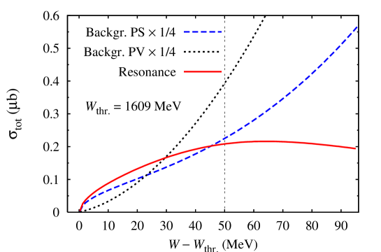
Figure 2: (Color online) Contribution of the background terms and the $S_{11}(1650)$ resonance amplitudes to the total cross section for the PS and PV couplings. Note that contribution of the $S_{11}(1650)$ resonance is the same in both couplings since the resonance parameters are fixed to the PDG values Amsler:2009 . The vertical line at 50 MeV above the production threshold indicates the upper limit of the energy of the present analysis.

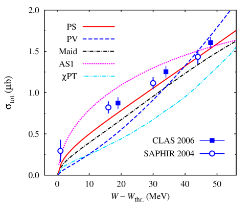
Figure 3: (Color online) Comparison between total cross sections calculated from the PS, PV, AS1 Adelseck:1990ch , and Kaon-Maid kaon-maid models with the result of the chiral perturbation theory ($\chi$PT) Steininger:1996xw and available experimental data from the SAPHIR Glander:2003jw and CLAS Bradford:2005pt collaborations. Note that all data shown in this figure were not used in the fitting process of the PS, PV, and Kaon-Maid models.

To investigate the role of the nucleon resonance $S_{11}(1650)$ in kaon photoproduction near threshold we compare contribution of this resonance with contributions of the backgrounds of the PS and PV models to the total cross section in Fig. 2. It is found that the $S_{11}(1650)$ contributes more than 20% to the total cross section in the PS model. In the PV model its contribution varies from about 15% up to 70%, depending on the energy. In Ref. Mart:2006dk it is shown that this resonance is only significant in the model that fits to the SAPHIR data, in which around 20% of the total cross section comes from the contribution of this resonance. In the model that fits to the CLAS data, the effect of this resonance is negligible (see Fig. 13 of Ref. Mart:2006dk ). Note that the background terms of the multipole model presented in Ref. Mart:2006dk ) is based on the PS coupling. We also note that the background contribution of PV model starts to dramatically increase at $W=25$ MeV above the threshold, as shown in Fig. 2. This indicates the deficiency of the PV model at higher energies, as clearly shown in Fig. 3. In previous analyses it was found that the deficiency of the PV model is caused by the fact that its background terms are found to be too large compared to those of the PS model bennhold:1987 ; Cheoun:1996kn ; thom . Our result is therefore consistent with previous analyses. Furthermore, from Fig. 2 we found that between threshold and $W=25$ MeV the PV background terms surprisingly yield smaller contribution to the cross section. Thus, very close to threshold the use of SU(3) main coupling constants should be also acceptable in the PV model.

V.2 Comparison with Experimental Data

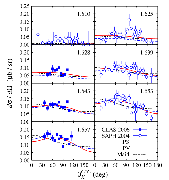
Figure 4: (Color online) Comparison between angular distributions of differential cross section calculated from the PS, PV, and Kaon-Maid kaon-maid models with experimental data from the SAPHIR Glander:2003jw and CLAS Bradford:2005pt collaborations. The corresponding total c.m. energy $W$ (in GeV) is shown in each panel. Experimental data displayed in this figure were used in the fits of the PS and PV models.

In Fig. 3 we compare total cross sections predicted by the PS, PV, AS1, and Kaon-Maid kaon-maid models with experimental data and prediction of the chiral perturbation theory Steininger:1996xw . Obviously, the PS model is the best model for kaon photoproduction near threshold. The PV result underestimates the data up to $W=40$ MeV above threshold. Kaon-Maid underpredicts the data by about 20% in the whole energy region of interest. The similar phenomenon is also shown by the prediction of chiral perturbation theory, i.e., it also underpredicts experimental data by about 30% - 50%. Interestingly, we observe that the prediction of the PV model is very close to the prediction of the chiral perturbation theory up to $W=10$ MeV above threshold. This fact originates from the small background terms of the PV model in this energy region, as discussed in the previous subsection. The AS1 model seems to overestimate most of the experimental data shown. Note that we did not use these total cross section data in our fits, because they are less accurate than the differential ones. Especially in the case of the CLAS data, where the angular distribution coverage is more limited than in the case of SAPHIR data.

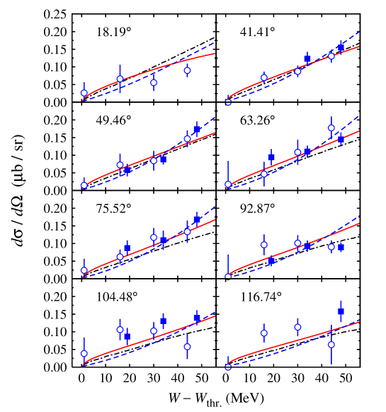
Figure 5: (Color online) As in Fig. 4, but for the total c.m. energy distribution. The corresponding kaon scattering angle $\theta_{K}^{\rm c.m.}$ is shown in each panel.

The angular distribution of differential cross section shows a certain structure (see Fig. 4). This structure is more obvious in the case of SAPHIR data. This structure seems to be missing in the Kaon-Maid, as clearly seen at $W=1.653$ MeV and 1.657 MeV. We also note that both AS1 and AS2 cannot produce this structure. Nevertheless, due to their limited accuracies, present experimental data do not allow for further analysis of this structure. Even the difference between the PS and PV models cannot be resolved at present. Therefore, for investigation of kaon photoproduction near threshold, experimental measurement of differential cross section with an accuracy of about 5% in the whole angular distribution is recommended. Especially important is the production at threshold, where isobar models seem to produce constant and structureless differential cross sections.

The energy distribution of differential cross section is shown in Fig. 5. Here we see that the agreement between model calculations and experimental data is quite satisfactory. The small deviations at $\theta_{K}^{\rm c.m.}=104.48^{\circ}$ and $116.74^{\circ}$ originate from the influence of backward angles data, specifically from SAPHIR data (see Fig. 4), which decrease the cross section at this kinematics during the fitting process.

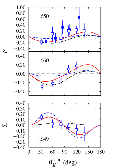
Figure 6: (Color online) Recoil polarization $P$ and photon asymmetry $\Sigma$ calculated from the PS, PV, and Kaon-Maid models kaon-maid compared with experimental data from the SAPHIR Glander:2003jw (open circles), CLAS Bradford:2005pt (solid squares), and GRAAL lleres07 (open squares) collaborations. Notation for the curves is as in Fig. 4. The corresponding total c.m. energy $W$ (in GeV) is shown in each panel.

The results for recoil polarization and photon asymmetry observables are shown in Fig. 6. It is widely known that these observables are quite sensitive to the choice of the resonance configuration. Again, we see that the agreement of the PS model is better than both PV and Kaon-Maid models.

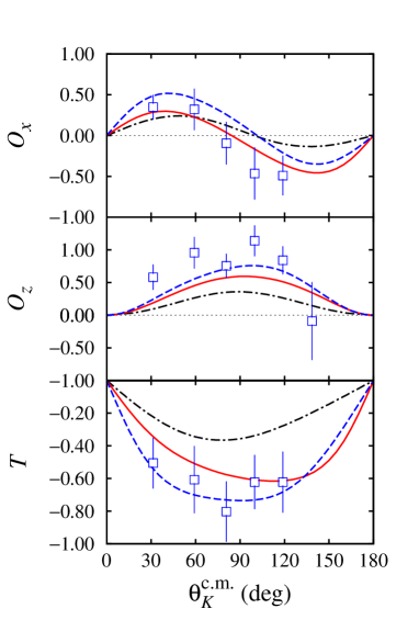
Figure 7: (Color online) The beam-recoil double polarization observables $O_{x}$ and $O_{z}$, along with target asymmetry $T$ predicted by the PS, PV, and Kaon-Maid models kaon-maid compared with experimental data from the GRAAL lleres09 collaboration. Notation of the curves is as in Fig. 4. Note that all experimental data shown in this figure were not used in the fitting process of all models.

V.3 The Beam-Recoil and Target Polarizations

The new experimental data for the beam-recoil and target polarizations have been recently released by the GRAAL collaboration lleres09 . These data require special attention because their definition of coordinate systems is slightly different from ours. The GRAAL data are obtained by using the coordinate system used by Adelseck and Saghai Adelseck:1990ch . In the present work we used the coordinate system of Knöchlein et al. germar . We note that the difference between the two coordinate systems leads to different signs of both $O_{x}$ and $O_{z}$ observables, but the same sign of the target asymmetry $T$. At this stage, it is important to remind the reader that already in the ”classical” paper of Barker, Donnachie and Storrow in 1975 Barker:1975bp a clear definition of signs and coordinate systems for this purpose has been given. In the work of Knöchlein et al germar these coordinate systems have been adopted. However, in the recent work of Sandorfi et al. Sandorfi:2009xe new expressions that allow a direct calculation of matrix elements with arbitrary spin projections are presented and used to clarify sign differences that exist in the literature. By comparing with Kaon-Maid (as well as SAID), it is found that within this convention the implied definition of six double-polarization observables, i.e. $H$, $L_{x^{\prime}}$, $C_{x^{\prime}}$, $C_{z^{\prime}}$, $O_{x^{\prime}}$, and $O_{z^{\prime}}$, are the negative of what has been used in comparing to recent experimental data. To comply with this finding we do not flip the original sign of the experimental data of the GRAAL collaboration lleres09 as shown in Fig. 7. Note that the data shown in Fig. 7 are not used in our analysis. Therefore, the calculated polarization observables shown here are pure prediction. Surprisingly, the predicted $O_{x}$ and $O_{z}$, as well as the target asymmetry $T$, are in perfect agreement with experimental data. This is true for both PS and PV models, although the presently available data cannot resolve the difference between the two models. We observe that the present calculation is still consistent with the result of Kaon-Maid model kaon-maid . We have also compared our result for the $O_{x}$ observable with that obtained by Adelseck and Saghai (see Fig. 11 of Ref. Adelseck:1990ch ) and found that our result is also consistent, especially at the backward direction, where the sign of $O_{x}$ becomes negative. To conclude this subsection, we would like to say that our result corroborates the finding of Sandorfi et al. Sandorfi:2009xe .

V.4 Effects of the Hyperon Resonance

The importance of the hyperon resonance in the background amplitude of isobar model for kaon photoproduction was pointed out by Adelseck and Saghai Adelseck:1990ch . They used the $S_{01}(1670)$ resonance in the AS1 model and the $S_{01}(1405)$ in the AS2 model (see Table 3). By including $S_{01}(1405)$ or $S_{01}(1670)$ they were able to fit the hitherto available experimental data and simultaneously reproduce the SU(3) values of main coupling constants $g_{K\Lambda N}$ and $g_{K\Sigma N}$. Later, Janssen et al. Janssen:2001wk found that the use of hyperon resonances $S_{01}(1800)$ and $P_{01}(1810)$, simultaneously, is desired in order to obtain the hadronic form factor cut-off greater than 1500 MeV in their model. The larger value of cut-off is desired in the kaon photoproduction because they argued that the value of $800$ MeV found in Ref. missing-d13 is rather unrealistic. In contrast to this, Kaon-Maid does not use any hyperon resonance in its background terms.

Table 4: Effects of the hyperon resonance inclusion on the total $\chi^{2}$ obtained from fits to the photoproduction data.

Resonance	-	$S_{01}(1405)$	$S_{01}(1670)$	$S_{01}(1800)$	$S_{11}(1750)$
$\chi^{2}$	189.4	136.7	135.7	127.9	133.7

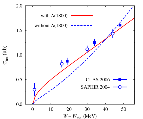
Figure 8: (Color online) Effect of the hyperon resonance $\Lambda(1800)$ inclusion on the total cross sections in the PS model.

In the present work we have tested the sensitivity of our fits to all four hyperon resonances listed in Table 1. The values of $\chi^{2}$ obtained from these fits are listed in Table 4. It is obvious that significant improvement in the $\chi^{2}$ would be obtained once we included this resonance, especially when the $S_{01}(1800)$ is used. This result corroborates the finding of Janssen et al. Janssen:2001wk , since the large hadronic cut-off requires another mechanism to damp the cross section at high energies. This is achieved by a destructive interference between the hyperon resonance contribution and other background terms. Such an interference is also observed in the present work, as obviously indicated by the total cross sections in Fig. 8. Although underpredicts experimental data at $W-W_{\rm thr}<40$ MeV, the model that excludes the $S_{01}(1800)$ resonance starts to overpredict the data, and therefore starts to diverge, at $W-W_{\rm thr}>40$ MeV.

The improvement obtained by including this resonance is not only observed in the total as well as differential cross sections, but also found in the calculated recoil polarizations and the target asymmetry as shown in Fig. 9. It is obvious from this figure that including this hyperon resonance results in a perfect agreement between our PS model and experimental data, especially the SAPHIR and GRAAL ones.

Figure 9: (Color online) Effect of the hyperon resonance $\Lambda(1800)$ inclusion on the recoil polarization and target asymmetry in the PS model. Notation of the curves is as in Fig. 8. Experimental data are as in Fig. 6.

VI Constraint from Kaon Electroproduction

For a polarized electron beam with helicity $h$ and no target or recoil polarization, the cross section of kaon electroproduction on a nucleon can be written as

$$\frac{d\sigma_{v}}{d\Omega_{K}} = \frac{d\sigma_{\rm T}}{d\Omega_{K}}+\epsilon\,\frac{d\sigma_{\rm L}}{d\Omega_{K}}+\epsilon\,\frac{d\sigma_{\rm TT}}{d\Omega_{K}}\cos 2\Phi+\sqrt{\epsilon(1+\epsilon)}\,\frac{d\sigma_{\rm LT}}{d\Omega_{K}}\,\cos\Phi$$ (14)

$$+h\sqrt{\epsilon(1-\epsilon)}\,\frac{d\sigma_{\rm LT^{\prime}}}{d\Omega_{K}}\,\sin\Phi~{},$$

where $\Phi$ is the angle between the electron (scattering) and hadron reaction planes, and $\epsilon$ is the transverse polarization of the virtual photon

$$\epsilon=\biggl{(}1-\frac{2{\bf k}^{2}}{k^{2}}\tan^{2}(\psi/2)\biggr{)}^{-1}~{},$$ (15)

with $\psi$ the electron scattering angle. All kinematical variables given in Eqs. (14) and (15) are shown in Fig. 10.

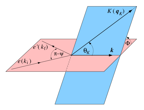
Figure 10: (Color online) Kinematic variables for kaon electroproduction on nucleons.

The subscripts T, L, and TT in Eq. (14) stand for transversely unpolarized, longitudinally polarized, and transversely polarized virtual photons. The subscripts LT and LT’ refer to the interference between transversely and longitudinally polarized virtual photons. Although they are generated by the same interference between longitudinal and transverse components of the hadronic and leptonic currents, they are different because they are generated by the real and imaginary parts of this interference term, respectively. The individual terms may be expressed in terms of the functions $A_{i}$ calculated in Sections II–IV.

In the following discussion we adopt the notation of Refs. Ambrozewicz:2006zj ; Nasseripour , i.e.

$$\sigma_{\rm T} = \frac{d\sigma_{\rm T}}{d\Omega_{K}}\,,$$ (16a)

$$\sigma_{\rm L} = \frac{d\sigma_{\rm L}}{d\Omega_{K}}\,,$$ (16b)

$$\sigma_{\rm U} = \sigma_{\rm T}+\epsilon\,\sigma_{\rm L}\,,$$ (16c)

$$\sigma_{\rm TT} = \frac{d\sigma_{\rm TT}}{d\Omega_{K}}\,,$$ (16d)

$$\sigma_{\rm LT} = \frac{d\sigma_{\rm LT}}{d\Omega_{K}}\,,$$ (16e)

$$\sigma_{\rm LT^{\prime}} = \frac{d\sigma_{\rm LT^{\prime}}}{d\Omega_{K}}\,,$$ (16f)

where $\sigma_{\rm U}$ refers to the unpolarized differential cross section.

The important ingredients in the electroproduction process are the electromagnetic form factors. Traditionally, to extend a photoproduction model to the case of virtual photon we may use the same hadronic coupling constants extracted from photoproduction data and put the appropriate electromagnetic form factors in the electromagnetic vertices. Since we are not in the position to investigate the effect of electromagnetic form factors in the kaon electroproduction process we use the standard Dirac and Pauli form factors for the proton, expressed in terms of the Sachs form factors,

$$F_{1}^{p}(Q^{2}) = \biggl{[}G_{E}(Q^{2})+\frac{Q^{2}}{4m_{p}^{2}}G_{M}(Q^{2})\biggr{]}\biggl{(}1+\frac{Q^{2}}{4m_{p}^{2}}\biggr{)}^{-1}~{},$$ (17a)

$$F_{2}^{p}(Q^{2}) = \biggl{[}G_{M}(Q^{2})-G_{E}(Q^{2})\biggr{]}\biggl{[}\kappa_{p}\biggl{(}1+\frac{Q^{2}}{4m_{p}^{2}}\biggr{)}\biggr{]}^{-1}~{},$$ (17b)

where $\kappa_{p}$ is the anomalous magnetic moment of the proton and $Q^{2}=-k^{2}$. In the momentum transfer region of interest, the Sachs form factors of the proton $G_{E}^{p}(Q^{2})$ and $G_{M}^{p}(Q^{2})$ can be described by the standard dipole form

$$G_{E}^{p}(Q^{2}) = \frac{G_{M}^{p}(Q^{2})}{1+\kappa_{p}}~{}=~{}\left(1+\frac{Q^{2}}{0.71~{}{\rm GeV}^{2}}\right)^{-2}~{}.$$ (18)

The kaon form factor is taken from the work of Cardarelli et al. cardarelli , i.e.

$$F^{K^{+}}(Q^{2})=\frac{a}{1+Q^{2}/\Lambda_{1}^{2}}+\frac{1-a}{(1+Q^{2}/\Lambda_{2}^{2})^{2}},$$ (19)

with $a=0.398$, $\Lambda_{1}=0.642$ GeV, and $\Lambda_{2}=1.386$ GeV. We note that this form factor has been used in the calculation of kaon electroproduction in Ref. david . For kaon resonances $K^{*}$ and $K_{1}$ we use the standard monopole form factor

$$F^{K^{*}}(Q^{2})=\left(1+\frac{Q^{2}}{\Lambda_{K^{*}}^{2}}\right)^{-1}~{}~{}~{}~{}~{},~{}~{}~{}~{}~{}F^{K_{1}}(Q^{2})=\left(1+\frac{Q^{2}}{\Lambda_{K_{1}}^{2}}\right)^{-1}~{},$$ (20)

where the cutoffs $\Lambda_{K^{*}}$ and $\Lambda_{K_{1}}$ are considered as free parameters. On the other hand for the form factors of hyperon and hyperon resonances we adopt the standard dipole form

$$F^{Y}(Q^{2})=\left(1+\frac{Q^{2}}{\Lambda_{Y}^{2}}\right)^{-2}~{}~{}~{}~{},~{}~{}~{}~{}F^{Y^{*}}(Q^{2})=\left(1+\frac{Q^{2}}{\Lambda_{Y^{*}}^{2}}\right)^{-2}~{},$$ (21)

where $\Lambda_{Y}$ and $\Lambda_{Y^{*}}$ are fitted to experimental data. In the case of PV coupling we also assume a monopole form as in Eq. (20) for the electromagnetic form factor in the contact diagram vertex. Finally, the dependence of the electric and scalar multipoles on $Q^{2}$ is taken as hanstein99

$$E_{0+}(W,Q^{2}) = E_{0+}(W)(1+\alpha Q^{2})\exp(-\beta Q^{2})~{},$$ (22a)

$$S_{0+}(W,Q^{2}) = S_{0+}(W)(1+\alpha Q^{2})\exp(-\beta Q^{2})~{},$$ (22b)

where $\alpha$ and $\beta$ are extracted from the fitting process.

We note that there are no kaon electroproduction data available very close to threshold. The lowest energy where the latest experiment has been performed at JLab is $W=1.65$ GeV. In fact, this value comes from the bin center of the collected data with $W$ spans from 1.60 GeV to 1.70 GeV Ambrozewicz:2006zj . The extracted data are $\sigma_{\rm U}$, $\sigma_{\rm TT}$, $\sigma_{\rm LT}$, which in total consist of 108 data points at $W=1.65$ GeV and $Q^{2}=0.65-2.55$ GeV². In addition, there have been also data available for the polarized structure function $\sigma_{\rm LT^{\prime}}$. To this end there are 12 extracted points at the same $W$ with $Q^{2}=0.65$ GeV² and $1.00$ GeV² Nasseripour .

Surprisingly, fitting the 120 electroproduction data points by adjusting 7 longitudinal parameters given above, i.e., $S^{0}_{1/2+}(p)$, $\alpha$, $\beta$, $\Lambda_{Y}$, $\Lambda_{Y_{3}^{*}}$, $\Lambda_{K^{*}}$ and $\Lambda_{K_{1}}$, is almost impossible, since in this case we obtain $\chi^{2}/N\approx 4000$. We have checked our Fortran code and found that this is caused by the large contribution from the background as the momentum transfer $Q^{2}$ increases, especially from the $K^{*}$ and $K_{1}$ intermediate states. There is of course many possible ways to limit their contributions. One of them is by introducing the same form factor as the one we have used in the multipoles. Thus, for instance, the $K^{*}$ intermediate state has

$$F^{K^{*}}(Q^{2}) = (1+\alpha_{K^{*}}Q^{2})\exp(-\beta_{K^{*}}Q^{2})~{}.$$ (23)

The result is shown in Table 5, where we have also used this form factor [Eq. (23)] in the ${Y_{3}^{*}}$ intermediate state, in order to obtain the lowest $\chi^{2}$.

Table 5: Extracted parameters from fit to electroproduction data (PS) and to both electroproduction and photoproduction data bases (PS1). The hadronic coupling constants in the PS model (marked with $\dagger$) were obtained from fit to photoproduction data and are fixed during the fit to electroproduction data. All fits use the PS coupling and the SU(3) predictions of the main coupling constants, $g_{K\Lambda N}/\sqrt{4\pi}=-3.80$ and $g_{K\Sigma N}/\sqrt{4\pi}=1.20$.

Coupling Constants	PS	PS1
$G^{V}_{K^{*}}/4\pi$	$-0.65^{\dagger}~{}$	$-0.13~{}~{}$
$G^{T}_{K^{*}}/4\pi$	$0.29^{\dagger}$	$-0.07~{}~{}$
$G^{V}_{K_{1}}/4\pi$	$0.42^{\dagger}$	$0.06$
$G^{T}_{K_{1}}/4\pi$	$-3.17^{\dagger}~{}$	$-0.04~{}~{}$
$G_{Y_{3}^{*}}/\sqrt{4\pi}$	$-4.93^{\dagger}~{}$	$-5.00~{}~{}$
$\phi$ (deg)	$218^{\dagger}$	322
$S_{1/2+}(p)$ ($10^{-3}$ GeV-1/2)	21.4	$-29.0~{}~{}$
$\alpha$ (GeV-2)	4.62	$3.10$
$\beta$ (GeV-2)	1.13	$0.97$
$\Lambda_{Y}$ (GeV)	1.10	$0.85$
$\alpha_{Y_{3}^{*}}$ (GeV-2)	0.76	-
$\beta_{Y_{3}^{*}}$ (GeV-2)	1.75	-
$\alpha_{K^{*}}$ (GeV-2)	0.00	-
$\beta_{K^{*}}$ (GeV-2)	5.50	-
$\alpha_{K_{1}}$ (GeV-2)	0.00	-
$\beta_{K_{1}}$ (GeV-2)	5.50	-
$\Lambda_{Y_{3}^{*}}$ (GeV)	-	$0.73$
$\Lambda_{K^{*}}$ (GeV)	-	$1.74$
$\Lambda_{K_{1}}$ (GeV)	-	$1.99$
$\chi^{2}/N$	1.27	1.22

As shown in the second column of Table 5, fitting the 120 electroproduction data points by adjusting 7 longitudinal parameters leads to non-conventional electromagnetic form factors of $K^{*}$ and $K_{1}$, because they practically have the form of $e^{-5.5Q^{2}}$. Note that the choice of the upper limit 5.5 is clearly trivial. However, it would not substantially change the conclusion if we increased it, since in the fitting process this value will always increase to the upper limit with only small effect on the $\chi^{2}$. Therefore, the use of the exponential type of form factor given by Eq. (23) will in principle remove contributions of the $K^{*}$ and $K_{1}$ intermediate states at finite $Q^{2}$.

If we compare the extracted $K^{*}$ and $K_{1}$ coupling constants from fit to photoproduction data (second columns of Tables 5 and 3 with those from previous work of Adelseck-Saghai Adelseck:1990ch (fourth and fifth columns of Table 3), we may conclude that the extracted coupling constants in the present work are consistent. However, compared to the work of Williams et al williams and Cheoun et al. Cheoun:1996kn (sixth and seventh columns of Table 3), it is found that the extracted couplings of the present work are much larger. In view of this, we think that it is necessary to refit the hadronic coupling constants in a simultaneous fit to both photo- and electroproduction data bases. In this case the electroproduction data will also influence the values of the extracted hadronic coupling constants. The result is shown in the third column of Table 5 and hereafter is called PS1. From this result it is obvious that the $K^{*}$ and $K_{1}$ coupling constants desired by the electroproduction data are much smaller than those extracted from the photoproduction data and, surprisingly, are of the order of those obtained by Williams et al. williams and Cheoun et al. Cheoun:1996kn .

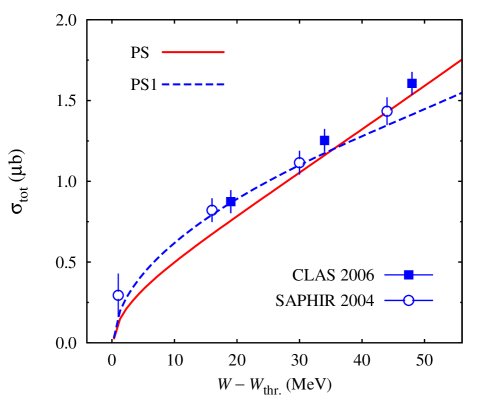
Figure 11: (Color online) Effect of the fitting to both photo- and electroproduction data simultaneously on the photoproduction total cross section. Solid line shows the calculated cross section from the PS model, discussed in Section V. Dashed line (PS1) displays the result of fitting to both photo- and electroproduction data, simultaneously.

The effect of fitting to both photo- and electroproduction data simultaneously on the photoproduction total cross section is displayed in Fig. 11. It is easy to understand that the effect of electroproduction data is more apparent in the “higher” energy region, since the data exist at $W=1.65$ GeV, about 40 MeV above the threshold. In this region, the cross section is suppressed due to the size of the electroproduction data, which are presumably much smaller than those expected by the photoproduction data. Interestingly, at “lower” energies, the agreement with experimental data is improved after including the electroproduction data.

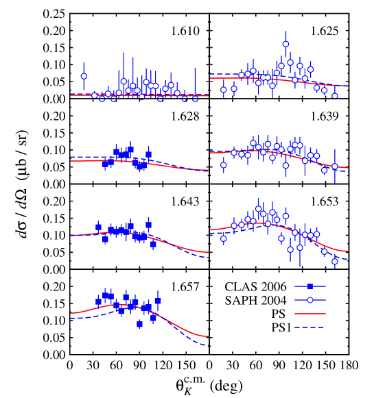
Figure 12: (Color online) As in Fig. 11, but for the angular distributions of the differential cross section. Experimental data are the same as those shown in Fig. 4.

To further elucidate the role of electroproduction data on the suppression of cross sections at $Q^{2}=0$ we display the angular distribution of the photoproduction differential cross section in Fig. 12. It is found that the suppression phenomenon occurs only at forward and backward angles (see panels with $W=1.653$ GeV and $W=1.657$ GeV). This phenomenon obviously originates from the small values of the $K^{*}$ and $K_{1}$ coupling constants. Unfortunately, experimental data from CLAS collaboration ($W=1.657$ GeV) are unavailable at these kinematical regions. The SAPHIR data at $W=1.653$ GeV seem to be better in this case. Nevertheless, the corresponding accuracy is still unable to firmly resolve the difference between the two calculations, although at the very forward and backward directions the data seem to favor the small values of the $K^{*}$ and $K_{1}$ coupling constants. Future experimental measurement at MAMI is expected to settle this problem.

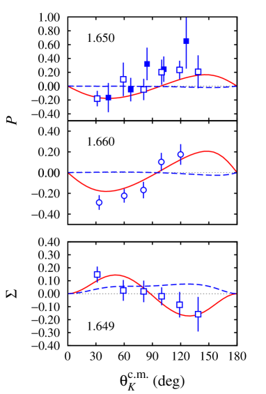
Figure 13: (Color online) As in Fig. 12, but for the angular distributions of the photon beam and recoil polarizations. Experimental data are the same as those shown in Fig. 6.

It is also important to note that by comparing the calculated photon beam and recoil polarizations with experimental data as shown in Fig. 13 we can observe the deficiency of the PS1 model. This is understandable, since the data shown in this figure are measured at $W\approx 1.65$ GeV, an energy region where predictions of the PS1 model for photoproduction are no longer reliable, due to the strong influence of the electroproduction data (see Fig. 11). Furthermore, the number of the polarization data in the fitting database cannot compete with that of the cross section data. Increasing the number and improving the accuracy of these data near the threshold or using the weighting factor in the fitting process could be expected to improve this situation.

A comparison between separated differential cross sections $\sigma_{\rm U}$, $\sigma_{\rm TT}$, and $\sigma_{\rm LT}$ calculated from the PS, PS1, and Kaon-Maid models with experimental data is shown in Fig. 14. In this case it is clear that the PS and PS1 can nicely reproduce the data and their difference is hardly seen. The same result is also shown in case of the polarized structure function $\sigma_{\rm LT^{\prime}}$, as displayed in Fig. 15. However, we notice that Kaon-Maid is unable to reproduce the available data in all cases and, in fact, it shows a backward peaking behavior for $\sigma_{\rm U}$, in contrast to the result of experimental measurement. We suspect that this behavior originates from the large contributions of the $K^{*}$ and $K_{1}$ intermediate states (see the fourth column of Table 3). In the PS or PS1 model their contributions are significantly suppressed by means of the exponential form factors or small values of $K^{*}$ and $K_{1}$ coupling constants, respectively.

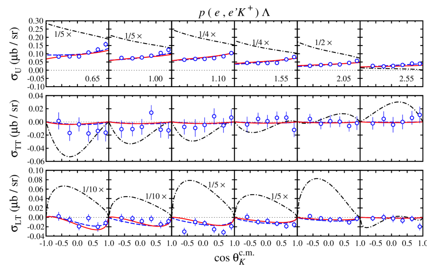
Figure 14: (Color online) Separated differential cross sections for kaon electroproduction $e+p\to e^{\prime}+K^{+}+\Lambda$ as a function of the kaon scattering angles at $W=1.65$ GeV and for different values of $Q^{2}$ (the values are shown in the top panels). Experimental data are from the CLAS collaboration Ambrozewicz:2006zj . Solid lines are due to the PS model, dashed lines show the result of the PS1 model, whereas dash-dotted lines display the predictions of Kaon-Maid. Note that predictions of Kaon-Maid in some panels have been renormalized by certain factors in order to fit on the scale.

It is also important to note that both PS and PV model seem to choose the zero $\sigma_{\rm TT}$, a conclusion that has been also drawn in Ref. Ambrozewicz:2006zj . However, we notice that this is in contrast to the prediction of Kaon-Maid.

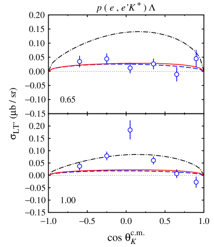
Figure 15: (Color online) Polarized structure function $d\sigma_{\rm LT^{\prime}}/{d\Omega}$ of the $e+p\to e^{\prime}+K^{+}+\Lambda$ channel as a function of the kaon scattering at $W=1.65$ GeV with $Q^{2}=0.65$ GeV² (upper panels) and $Q^{2}=1.00$ GeV² (lower panels). Notation of the curves is as in Fig. 14. Experimental data are from Ref. Nasseripour .

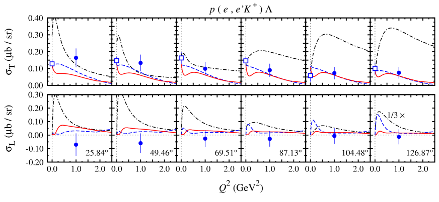
Figure 16: (Color online) Separated transverse (upper panels) and longitudinal (lower panels) differential cross sections of the $e+p\to e^{\prime}+K^{+}+\Lambda$ channel as a function of the virtual photon momentum transfer $Q^{2}$ at $W=1.65$ GeV and different $\theta_{K}^{\rm c.m.}$ (shown in lower panels). Notation of the curves is as in Fig. 14. Experimental data of electroproduction at $Q^{2}=1.0$ GeV² (solid circles) are from Ref. Ambrozewicz:2006zj , whereas data of photoproduction (open squares) are due to the SAPHIR collaboration Glander:2003jw . Note that predictions of Kaon-Maid have been renormalized by a factor 1/3 in the lower panels in order to fit on the scale. The electroproduction data shown in this figure are not used in our calculation.

The $Q^{2}$ evolution of the longitudinal cross section $\sigma_{\rm L}$ is of special interest, especially for estimating the possibility of extracting kaon form factor $F_{K}(Q^{2})$. In the latest measurement at JLab there has been an attempt to separate $\sigma_{\rm L}$ and $\sigma_{\rm T}$ from $\sigma_{\rm U}$. Except at $W=1.95$ GeV results of both the Rosenbluth and the simultaneous $\epsilon-\Phi$ fit techniques are plagued with the “nonphysical” (negative) longitudinal cross section $\sigma_{\rm L}$. Nevertheless, it was concluded that within the combined systematical and statistical uncertainties the longitudinal cross sections are believed to be zero Ambrozewicz:2006zj .

The result of our PS and PS1 models are compared with the prediction of Kaon-Maid and very limited experimental data in Fig. 16. The agreement of the PS and PS1 models with the photoproduction data for transverse cross section at $Q^{2}=0$ is certainly not surprising. However, the discrepancies between experimental data and model calculations at $Q^{2}=1$ GeV² still show the consistency of the presented models. It should be remembered that both PS and PS1 models were fitted to the same, but unseparated data $\sigma_{\rm U}$. Therefore, as shown in upper and lower panels with the same $\theta_{K}^{\rm c.m.}$ in Fig. 16, the underpredicted $\sigma_{\rm T}$ will always be compensated by the overpredicted $\sigma_{\rm L}$. This result clearly indicates that in order to avoid the “nonphysical” separated longitudinal cross section $\sigma_{\rm L}$, a model-dependent extraction of $\sigma_{\rm L}$ and $\sigma_{\rm T}$ would be strongly recommended. Obviously, this could be performed only if we had a reliable isobar model that can describe all available data.

From the smallness of the longitudinal cross sections shown in Fig. 16, it is obvious that the extraction of $K^{+}$ form factor is difficult near the production threshold. Moreover, we have numerically found that the longitudinal cross sections shown in the lower panels of Fig. 16 are dominated by the $S_{11}(1650)$ contribution. This is understandable since these cross sections are calculated at $W=1.65$ GeV, precisely at the pole position. In Ref. Ambrozewicz:2006zj it is shown that the “physical” (positive) longitudinal cross section data are only found at higher $W$, i.e. 1.95 GeV. From this fact, the extraction of the kaon electromagnetic form factor is naturally recommended at higher energies. Especially at $W$ above 2 GeV, where the contribution of nucleon resonances becomes less significant than the background terms. Furthermore, the extraction is best performed at small $|t|$, i.e., forward angles, where the contribution of $t$-channel is maximum.

For completeness we would like also to mention that we have investigated also kaon electroproduction in the case of PV coupling and found no substantial difference from the result of PS coupling.

VII Summary and Conclusions

We have investigated kaon photo- and electroproduction off a proton near the production threshold by means of an isobar model. The background amplitude is constructed from the appropriate Feynman diagrams, whereas the resonance amplitude is calculated by using the multipole formalism. In contrast to the results of the previous works that utilize isobar model or chiral perturbation theory it is found that both PS and PV models in the present work can nicely describe the available photoproduction data up to $W=50$ MeV above the threshold. Since in this work the values of the main coupling constants $g_{K\Lambda N}$ and $g_{K\Sigma N}$ are fixed to the SU(3) symmetry prediction, the obtained $\chi^{2}$ in the PV model is larger than in the case of the PS model. This originates from the fact that for the same coupling constants, the background amplitudes of the PV model is larger than that of the PS model. The $K^{*}$ and $K_{1}$ coupling constants are found to be consistent with the previous works. The $\Lambda$ resonance $S_{01}(1800)$ is found to play an important role in improving the agreement of the model calculation with experimental data, especially in the case of photon and recoil polarizations.

It is found that the $K^{*}$ and $K_{1}$ hadronic coupling constants extracted from photoproduction data lead to very large electroproduction differential cross sections, and therefore could not be used unless special form factors that strongly suppress their contributions were introduced or the hadronic coupling constants were refitted to both photo- and electroproduction databases, simultaneously. In the latter, the model reliability at lower energies is improved, whereas at higher energies the calculated photoproduction observables significantly deviate from experimental measurement due to the strong influence of electroproduction data. From the size of longitudinal cross sections $\sigma_{\rm L}$ predicted by both PS and PS1 models we may conclude that investigation of the kaon electromagnetic form factor, that strongly relies on $\sigma_{\rm L}$, is difficult to perform near the threshold region. More accurate experimental data at this energy region would certainly help to clarify some uncertainties in the present work.

References

- (1) R. A. Adelseck, C. Bennhold, and L. E. Wright, Phys. Rev. C 32, 1681 (1985).
- (2) R. A. Adelseck and B. Saghai, Phys. Rev. C 42, 108 (1990).
- (3) R. A. Williams, C.-R. Ji, and S. R. Cotanch, Phys. Rev. C 43, 452 (1991).
- (4) B. S. Han, M. K. Cheoun, K. S. Kim and I. T. Cheon, Nucl. Phys. A 691, 713 (2001).
- (5) T. Mart, C. Bennhold, H. Haberzettl, and L. Tiator, Kaon-Maid. The interactive program is available at http://www.kph.uni-mainz.de/MAID/kaon/kaonmaid.html. The published versions are available in: Ref. missing-d13 ; T. Mart, Phys. Rev. C 62, 038201 (2000); C. Bennhold, H. Haberzettl and T. Mart, arXiv:nucl-th/9909022.
- (6) S. Janssen, J. Ryckebusch, D. Debruyne and T. Van Cauteren, Phys. Rev. C 65, 015201 (2001).
- (7) A. de la Puente, O. V. Maxwell and B. A. Raue, Phys. Rev. C 80, 065205 (2009).
- (8) T. Feuster and U. Mosel, Phys. Rev. C 59, 460 (1999).
- (9) W. T. Chiang, F. Tabakin, T. S. H. Lee and B. Saghai, Phys. Lett. B 517, 101 (2001).
- (10) V. Shklyar, H. Lenske and U. Mosel, Phys. Rev. C 72, 015210 (2005).
- (11) B. Julia-Diaz, B. Saghai, T. S. Lee and F. Tabakin, Phys. Rev. C 73, 055204 (2006).
- (12) A. V. Anisovich, V. Kleber, E. Klempt, V. A. Nikonov, A. V. Sarantsev and U. Thoma, Eur. Phys. J. A 34, 243 (2007).
- (13) M. Guidal, J. M. Laget and M. Vanderhaeghen, Nucl. Phys. A627, 645 (1997).
- (14) Z. P. Li, Phys. Rev. C 52, 1648 (1995).
- (15) D. H. Lu, R. H. Landau and S. C. Phatak, Phys. Rev. C 52, 1662 (1995).
- (16) T. Mart and T. Wijaya, Acta Phys. Polon. B 34, 2651 (2003).
- (17) T. Mart and C. Bennhold,“Kaon photoproduction in the Feynman and Regge theories,” arXiv:nucl-th/0412097.
- (18) T. Corthals, J. Ryckebusch and T. Van Cauteren, Phys. Rev. C 73, 045207 (2006).
- (19) P. Vancraeyveld, L. De Cruz, J. Ryckebusch and T. Van Cauteren, Phys. Lett. B 681, 428 (2009).
- (20) C. Amsler et al. (Particle Data Group), Phys. Lett. B 667, 1 (2008).
- (21) B. Saghai and F. Tabakin, Phys. Rev. C 53, 66 (1996).
- (22) J. Antolin, Z. Phys. C 31, 417 (1986).
- (23) M. Bozoian, J. C. G. van Doremalen, and H. J. Weber, Phys. Lett. 122B, 138 (1983).
- (24) S. Choe, M. K. Cheoun, and S. H. Lee, Phys. Rev. C 53, 1363 (1996).
- (25) H. Tanabe, M. Kohno, and C. Bennhold, Phys. Rev. C 39, 741 (1989).
- (26) K. H. Glander et al., Eur. Phys. J. A 19, 251 (2004).
- (27) R. Bradford et al. [CLAS Collaboration], Phys. Rev. C 73, 035202 (2006).
- (28) M. K. Cheoun, B. S. Han, I. T. Cheon and B. G. Yu, Phys. Rev. C 54, 1811 (1996).
- (29) M. E. McCracken et al., Phys. Rev. C 81, 025201 (2010)
- (30) D. Drechsel, O. Hanstein, S. S. Kamalov and L. Tiator, Nucl. Phys. A 645, 145 (1999).
- (31) L. Tiator, D. Drechsel, S. Kamalov, M. M. Giannini, E. Santopinto and A. Vassallo, Eur. Phys. J. A 19, 55 (2004).
- (32) P. Bydžovský and T. Mart, Phys. Rev. C 76, 065202 (2007).
- (33) B. B. Deo and A. K. Bisoi, Phys. Rev. D 9, 288 (1974).
- (34) P. Dennery, Phys. Rev. 124, 2000 (1961).
- (35) B. Pasquini, D. Drechsel and L. Tiator, Eur. Phys. J. A 34, 387 (2007).
- (36) T. Mart and A. Sulaksono, Phys. Rev. C 74, 055203 (2006).
- (37) G. Knöchlein, D. Drechsel, and L. Tiator, Z. Phys. A 352, 327 (1995).
- (38) I. S. Barker, A. Donnachie and J. K. Storrow, Nucl. Phys. B 95, 347 (1975).
- (39) A. M. Sandorfi, S. Hoblit, H. Kamano and T. S. Lee, “Calculations of Polarization Observables in Pseudoscalar Meson Photo-production Reactions,” arXiv:0912.3505 [nucl-th].
- (40) S. S. Hsiao, D. H. Lu, and S. N. Yang Phys. Rev. C 61, 068201 (2000).
- (41) A. Lleres et al., Eur. Phys. J. A 31, 79 (2007).
- (42) A. Lleres et al., Eur. Phys. J. A 39, 146 (2009).
- (43) C. Bennhold and L. E. Wright, Phys. Rev. C 36, 438 (1987).
- (44) S. Steininger and U. G. Meissner, Phys. Lett. B 391, 446 (1997).
- (45) H. Thom, Phys. Rev. 151, 1322 (1966).
- (46) T. Mart and C. Bennhold, Phys. Rev. C 61, 012201 (1999).
- (47) P. Ambrozewicz et al., Phys. Rev. C 75, 045203 (2007).
- (48) R. Nasseripour et al., Phys. Rev. C 77, 065208 (2008).
- (49) F. Cardarelli, I. L. Grach, I. M. Narodetskii, E. Pace, G. Salme, and S. Simula, Phys. Rev. D 53, 6682 1996.
- (50) J. C. David, C. Fayard, G. H. Lamot, and B. Saghai, Phys. Rev. C 53, 2613 (1996).