Dynamics of Neptune’s Trojans: II. Eccentric orbits and observed ones

Abstract

In a previous paper, we have presented a global view of the stability of Neptune Trojan (NT hereafter) on inclined orbit. As the continuation of the investigation, we discuss in this paper the dependence of stability of NT orbits on the eccentricity. For this task, high-resolution dynamical maps are constructed using the results of extensive numerical integrations of orbits initialized on the fine grids of initial semimajor axis ($a_{0}$) versus eccentricity ($e_{0}$). The extensions of regions of stable orbits on the ($a_{0},e_{0}$)- plane at different inclinations are shown. The maximum eccentricities of stable orbits in three most stable regions at low ($0^{\circ},12^{\circ}$), medium ($22^{\circ},36^{\circ}$) and high ($51^{\circ},59^{\circ}$) inclination, are found to be 0.10, 0.12 and 0.04, respectively. The fine structures in the dynamical maps are described. Via the frequency analysis method, the mechanisms that portray the dynamical maps are revealed. The secondary resonances, concerning the frequency of the librating resonant angle $\lambda-\lambda_{8}$ and the frequency of the quasi 2:1 mean motion resonance (MMR for short hereafter) between Neptune and Uranus, are found deeply involved in the motion of NTs. Secular resonances are detected and they also contribute significantly to the triggering of chaos in the motion. Particularly, the effects of the secular resonance $\nu_{8},\nu_{18}$ are clarified.

We also investigate the orbital stabilities of six observed NTs by checking the orbits of hundreds clones of them generated within the observing error bars. We conclude that four of them, except 2001 QR322 and 2005 TO74, are deeply inside the stable region. The 2001 QR322 is in the close vicinity of the most significant secondary resonance. The 2005 TO74 locates close to the boundary separating stable orbits from unstable ones, and it may be influenced by a secular resonance.

1 Introduction

Besides the trans-Neptunian region (also known as “Kuiper belt”) outside the orbit of Neptune and the “main belt” in between the orbits of Mars and Jupiter, the trojan-cloud around some planets is another main reservoir of minor objects in the Solar system. Thousands of Trojan asteroids orbiting around the equilateral Lagrange equilibrium points of Jupiter have been observed and catalogued since the discovery of (588) Achilles in 1906 [Nicholson 1961]. In recent years, six NTs were discovered and many more of them are expected in future [Sheppard & Trujillo 2006]. As for other planets, except for Mars, of which 4 Trojans are known, investigations show the evidences of large unstable areas around the triangular Lagrange points [Marzari, Tricarico & Scholl 2003a, Nesvorný & Dones 2002, Dvorak, Bazso & Zhou 2010].

Since the observed NTs show a wide range of orbital elements (especially the inclination, see Table 1) and the potential Trojan swarm could be much more thick than the one of Jupiter [Sheppard & Trujillo 2006], many studies have focused on this asteroid population, with interests both in the orbital dynamics and capturing history e.g., [Brasser et al. 2004, Zhou, Dvorak & Sun 2009a, Zhou, Dvorak & Sun 2009b, Li, Zhou & Sun 2007, Nesvorný & Vokrouhlický 2009, Lykawka et al 2009].

In a previous paper (Zhou, Dvorak & Sun 2009, hereafter Paper I), we investigated the orbital stability of massless artificial asteroids around the triangular Lagrange points of Neptune ($L_{4}$ and $L_{5}$) in a model consisting of the Sun and four outer planets (Jupiter, Saturn, Uranus and Neptune). We constructed the “dynamical maps” on the plane of initial semimajor axis versus inclination $(a_{0},i_{0})$ to study the dependence of stability on inclination. We confirmed two stable regions with inclination in the ranges of $(0^{\circ},12^{\circ})$ and $(22^{\circ},36^{\circ})$ [Nesvorný & Dones 2002], and found a new stable region for highly-inclined orbits with $i_{0}\in(51^{\circ},59^{\circ})$.

To complete the investigation of orbital stability in the whole orbital parameter space, we present in this paper a detailed analysis on the dependence of orbital stability on the initial eccentricity. We will explain the dynamical model, numerical algorithm and analytical method used in this paper in Section 2. The main results will be given in Section 3, where the dynamical maps on the plane of $(a_{0},e_{0})$ are plotted and described. Then in Section 4, through a frequency analysis method, we will discuss the mechanisms that sculpture the dynamical maps. In Section 5, the orbits of the 6 observed NTs will be checked and compared with our previous results. Finally, a summation and a discussion will be given in Section 6.

2 Model and Method

Basically, the dynamical model, the numerical method and the analytical tools used in this paper are the same or very similar to the ones in Paper I. We give a brief introduction below.

2.1 Dynamical model and analyzing methods

All the computations and analysis in this paper are under the “outer Solar system model” in which the massless fictitious asteroids orbit around Neptune’s triangular Lagrange points in the gravitation field of the Sun and the four outer giant planets. Since $L_{4}$ and $L_{5}$ are dynamically symmetrical to each other [Nesvorný & Dones 2002, Marzari, Tricarico & Scholl 2003a, Zhou, Dvorak & Sun 2009a], we may investigate only one of them without losing the generality. Below we will discuss only the trailing point $L_{5}$.

To simulate the orbital evolution, we use the Lie-series integrator [Hanslmeier & Dvorak 1984]. An on-line low-pass filter is embedded in to remove the short-term oscillations in the outputs [Michtchenko & Ferraz-Mello 1995, Michtchenko et al. 2002]. The spectra of each orbit are then calculated from these filtered outputs using the Fast Fourier Transform (FFT) method. The number of peaks above a given level in a spectrum is counted. This so-called “Spectral Number” (SN) can be regarded as an indicator of the regularity of an orbit [Michtchenko & Ferraz-Mello 1995, Michtchenko et al. 2002, Ferraz-Mello et al. 2005], and it is used to construct the dynamical maps on the initial orbital parameter plane. The frequencies obtained from the FFT procedure are also carefully analyzed to determine the mechanisms that portrait the features in the dynamical maps. For details of the above mentioned methods and technologies, please refer to Paper I.

2.2 Initial conditions and the libration center

In order to get representative initial conditions for numerical simulations, we follow a similar scheme as Nesvorný and Dones [Nesvorný & Dones 2002] did. The initial orbital elements of fictitious asteroids are taken from a grid on the plane $(a_{0},e_{0})$, where 101 values of the semimajor axes $a_{0}$ are chosen uniformly between 29.9 and 30.5 AU, and the eccentricities $e_{0}$ vary up from 0.0 to 0.5 with an increment of 0.005. For all orbits on the grid, the initial inclinations $i_{0}$ are fixed at a given value. The angular elements of the orbits, including the ascending node $\Omega_{0}$, the perihelion argument $\omega_{0}$ and the mean anomaly $M_{0}$, are arranged in such a way that the resonant angle $\sigma$ ($\sigma=\lambda-\lambda_{8}$, the difference between the mean longitudes of Neptune $\lambda_{8}$ and the fictitious trojan $\lambda$) is at the center of tadpole orbit ($\sigma_{c}\approx-60^{\circ}$). Specifically, we set $\Omega_{0}=\Omega_{8},\omega_{0}=\omega_{8}-60^{\circ}$ and $M_{0}=M_{8}+\sigma_{c}+60^{\circ}$.

It is known that the libration center $\sigma_{c}$ changes with the eccentricity and inclination. In the restricted three body model consisting of the Sun, Neptune and the Trojan, the value of $\sigma_{c}$ at a given eccentricity and inclination can be determined by locating the extremes of the averaged Hamiltonian (energy) on the $(\sigma,a)$ -plane [Nesvorný et al. 2002]. In the outer solar system model adopted in this paper, because of the perturbations from other planets, there could be no such a center with zero libration amplitude of $\sigma$. However, we can still locate the position at which $\sigma$ librates with the smallest amplitude. A series of orbits are integrated and the one with minimum libration amplitude is “defined” as the libration center.

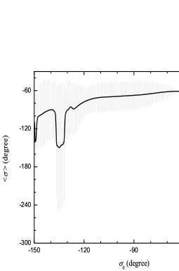
Figure 1: The mean value (solid curve) and the libration amplitude (error bars) of $\sigma$ versus initial $\sigma_{0}$. These 101 orbits have the same orbital elements except their mean anomalies differ from each other so that they have different initial resonant argument $\sigma_{0}$. The initial eccentricity and inclination of these orbits are $e_{0}=0.1,i_{0}=0^{\circ}$. The minimum of libration amplitude ($\Delta\sigma=6.97^{\circ}$) is at $\sigma_{c}=-64^{\circ}$.

In this series of orbits, the initial semimajor axes are chosen as the same value as Neptune’s, $a_{0}=a_{8}$ and $e_{0},i_{0}$ are given the specific values. The initial angular elements are given the representative value as mentioned above, $\omega_{0}=\omega_{8}-60^{\circ},\Omega_{0}=\Omega_{8},M_{0}=M_{8}+60^{\circ}+\sigma$. We test $\sigma$ in the range $(-100^{\circ},-50^{\circ})$. The orbits are then integrated up to $\sim 3.3\times 10^{5}$ yr, which is about 4 times longer than the typical long-term variation period of $\sigma$ [Murray & Dermott 1999]. We determine the “practical” libration center from the behaviour of the mean value and the librating amplitude of $\sigma$. An example with initial eccentricity $e_{0}=0.1$ and inclination $i_{0}=0^{\circ}$ is shown in Fig. 1.

It is interesting to notice in Fig. 1 that around the libration center the libration amplitude increases with the difference of the initial $\sigma_{0}$ from the center $\sigma_{c}$ and both of the mean value and oscillation amplitude change continuously, reflecting the regularity of motion around the libration center. When the initial $\sigma_{0}$ is far away from the center, e.g. $\sigma_{0}<-90^{\circ}$, the libration amplitude becomes large and the mean value changes randomly, indicating the chaotic character of motion.

Varying $e_{0},i_{0}$ and repeating the above calculations, we find the variation of libration center with respect to $e_{0}$ and $i_{0}$. A summation is plotted in Fig. 2 for orbits with initial conditions of $e_{0}=0-0.30$ and $i_{0}=0^{\circ}-60^{\circ}$. We ignore higher eccentricity and inclination because the highly eccentric and/or inclined orbits are unstable and therefore are of less interest. In fact, at very high eccentricity, the libration center may “bifurcate” to two centers. But this phenomenon is out of the range of current paper.

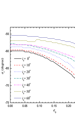
Figure 2: The variation of libration center ($\sigma_{c}$) with respect to eccentricity. From bottom to top, the curve represents the case for initial inclination from $0^{\circ}$ to $60^{\circ}$, respectively.

As shown in Fig. 2, the libration center of the tadpole orbit shifts farther away from Neptune as the eccentricity of the orbit increases. For the coplanar orbit ($i_{0}=0^{\circ}$), the libration center is exactly at the equilateral triangular point with $\sigma_{c}=-60^{\circ}$ when the eccentricity is 0, and it changes continuously to $\sigma_{c}\sim-71^{\circ}$ when the eccentricity increases to 0.25. The $\sigma_{c}$ also changes a little with respect to the inclination, and compared with coplanar orbits, the variation of $\sigma_{c}$ with eccentricity for highly inclined orbits becomes smaller.

Only after knowing the libration center $\sigma_{c}(e_{0},i_{0})$ at different eccentricity ($e_{0}$) and inclination ($i_{0}$), we can select the proper initial conditions to construct the representative dynamical maps. Namely, for a given inclination $i_{0}$, a dynamical map on the $(a_{0},e_{0})$- plane is constructed by analyzing the stability of each orbit on this plane and with other initial angular elements given by $\Omega_{0}=\Omega_{8},\omega_{0}=\omega_{8}-60^{\circ},M_{0}=M_{8}+60^{\circ}+\sigma_{c}(e_{0},i_{0})$.

3 Dynamical maps

We have investigated in Paper I the dependence of orbital stability of NT on the inclination. In this paper, we focus on the dependence of stability on the eccentricity. For this sake, the initial inclinations $i_{0}$ is fixed at given values and we study the orbits of the fictitious trojans initialized on the grid on the $(a_{0},e_{0})$- plane with other orbital elements determined in a way described in last section. Using the “spectra number” (SN) as the indicator of the regularity of an orbit as in Paper I, we construct dynamical maps on the $(a_{0},e_{0})-$ plane.

We present in Fig. 3 the dynamical maps for $i_{0}=0^{\circ},10^{\circ},20^{\circ},30^{\circ},40^{\circ}$ and $i_{0}=50^{\circ}$. The color in these dynamical maps indicates the orbital regularity. The green represents the most regular orbit, the red is on the edge of chaotic motion and the white indicates that the orbit does not survive on the trojan-like orbit in our numerical simulation (which lasts about 34 Myr). According to our experiences in Paper I, orbits with SN$>50$ (color blue) are not to be expected to survive in the Solar system age. Surely it is impossible and also unnecessary to calculate each slice at every possible initial inclination. These slices in Fig. 3 are enough to show the variation of dynamical map with respect to the initial inclination. We also discard those cases in which most of the trojan orbits are unstable and therefore less interested. For instance, due to the depletion effects arising from the $\nu_{8}$ secular resonance and Kozai resonance, the motion of trojans with $i_{0}\sim 45^{\circ}$ and $i_{0}>60^{\circ}$ are unstable (see Paper I), so that the dynamical maps are plain and not shown here. However, for the sake of providing more information about the trojan motion at other inclinations, other three dynamical maps for $i_{0}=5^{\circ},35^{\circ}$ and $55^{\circ}$ are used in Figs. 5, 6 & 7 as examples to present our frequency analysis in next section.

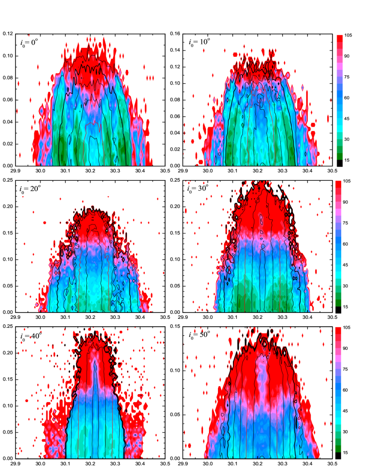
Figure 3: Dynamical maps on $(a_{0},e_{0})-$ plane, for initial inclinations $0^{\circ},10^{\circ},20^{\circ},30^{\circ},40^{\circ}$ and $50^{\circ}$ (left to right, top to bottom). The abscissae and ordinates are initial semimajor axes and eccentricities. Note the ordinates may have different scales. The contour curves represent the libration amplitude of resonant angle $\sigma=\lambda-\lambda_{8}$. From inside out are contours for $\Delta\sigma=10^{\circ}$ to $\Delta\sigma=70^{\circ}$ with an increment of $10^{\circ}$. Particularly, the red curves are for $\Delta\sigma=30^{\circ}$ and the thick ones represent $\Delta\sigma=60^{\circ}$.

The first conclusion drawn from these dynamical maps may be that the most stable motion (color green) does not happen at any inclination, but only at $i_{0}=0^{\circ},5^{\circ},10^{\circ},30^{\circ},35^{\circ}$ and $55^{\circ}$. This is consistent with the finding in Paper I of three most stable regions in inclination: Region A $(i_{0}=0^{\circ}-12^{\circ})$, B $(i_{0}=22^{\circ}-36^{\circ})$ and C $(i_{0}=51^{\circ}-59^{\circ})$.

A second conclusion is that the initial eccentricity $e_{0}$ for stable orbits must be small. Although for some initial inclinations (e.g. $i_{0}=30^{\circ},35^{\circ}$) some orbits with $e_{0}$ as large as 0.25 survive in our integrations and may survive even for much longer time, their SN’s (color red) indicate that most probably they will not remain on the trojan-like orbits in the Solar system age. These orbits with high $e_{0}$ may suffer perturbations through resonances whose effects appear significantly only in a timespan much longer than our integration time. For the most stable orbits, the largest initial eccentricities are around 0.08 in Region A, 0.07 in Region B and 0.02 in Region C. However, if we use a lenient criterion, namely, regarding all the orbits with SN$<50$ as survival ones (in the Solar system age), the permitted eccentricity extends to 0.10, 0.12 and 0.04 in Region A, B and C respectively. Out of these three most stable regions in inclination, there are also some narrow areas in which the motion is stable. For example, on the slice of $i_{0}=20^{\circ}$ in Fig. 3, we see a few stable orbits with $e_{0}<0.05$.

The contour of libration amplitude of the resonant angle $\Delta\sigma=\sigma_{\rm max}-\sigma_{\rm min}$ is also calculated and over-plotted on the dynamical maps. Clearly the relation between $\Delta\sigma$ and the deviation of semimajor axis from its mean value $a_{0}-a_{c}$ [Érdi 1988, Milani 1993, Zhou, Dvorak & Sun 2009a] is obeyed. The $\Delta\sigma$ increases monotonically with the distance of initial semimajor axis $a_{0}$ from its value at libration center ($a_{c}\sim 30.22$ AU). The maximum $\Delta\sigma$ is around $\Delta\sigma\sim 70^{\circ}$ for stable orbits with low (Region A) and medium inclination (Region B), but shrinks a little for high inclination (Region C) to $\Delta\sim 50^{\circ}$. At given $i_{0}$ and $a_{0}$, the libration amplitude increases only very little as the initial eccentricity increases. At high eccentricity, the $\Delta\sigma$ may still be small, but the large SN implies a chaotic motion. Therefore, the small libration amplitude manifested in our integration time may increase in a distant future. We also note that there is a lack of small $\Delta\sigma$ at some inclination values. For example, at $i_{0}=0^{\circ},10^{\circ}$ and $50^{\circ}$ all trojan orbits have $\Delta\sigma>10^{\circ}$. Last but not least, thanks to the calculation of libration center $\sigma_{c}$ and proper selection of initial conditions, both the dynamical maps and the libration amplitude contours have the bilaterally symmetrical features. Otherwise, if we just simply set $\sigma_{c}=-60^{\circ}$, these figures would be distorted.

Contrary to the profiles of the libration amplitude contours that are more or less plain, the dynamical maps bear plenty of fine structures. Most distinctly, there are vertical gaps of irregular motion on slices of small inclination ($i_{0}=0^{\circ},5^{\circ},10^{\circ}$), and a “spike” of relatively regular orbits with small $\Delta\sigma$ can be clearly seen on slices of large inclination ($i_{0}=40^{\circ},50^{\circ},55^{\circ}$). On one hand, these fine structures reveal the peculiar behaviour of orbits in these regions; on the other hand, they supply hints of the mechanisms taking effects and portraying the dynamical maps in the corresponding parameter space. We will try in next section to locate different kinds of resonances on the $(a_{0},e_{0})$- plane and compare them with the fine structures in the dynamical maps.

We would like to notify that the dynamical maps are plotted based on the osculating orbital elements in our papers. As we have shown in Paper I, the dynamical map would change if a different epoch was chosen. In a different epoch, the features of the dynamical map are very well kept, and the change is nothing more than a shift in the semimajor axis. If the proper libration amplitude and proper eccentricity, instead of the osculating semimajor axis and osculating eccentricity, are used to define the representative plane for the dynamical map, we may obtain the epoch-free dynamical maps as in [Marzari, Tricarico & Scholl 2003a, Marzari, Tricarico & Scholl 2003b, Dvorak et al. 2007]. But the osculating elements have the merit of being able to compare with the observing data directly. To do this, all we need is to transform the observing data to the corresponding epoch, as we will do in Section 5 of this paper.

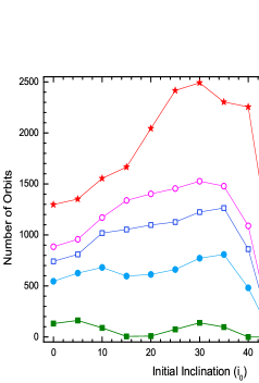
Figure 4: The number of regular orbits versus the initial inclination. From bottom up, the solid squares, solid circles, open squares, open circles and stars indicate the numbers of orbits whose SN’s are smaller than 25, 45, 65, 85 and 105. Remember all those orbits with original ${\rm SN}>100$ and $29.9\,{\rm au}<\bar{a}<$ 30.5 au are assigned a new SN of 100 (please refer to Paper I for details).

We have calculated many other dynamical maps with different initial inclinations, of which three maps for $i_{0}=5^{\circ},35^{\circ}$ and $i_{0}=55^{\circ}$ are going to be shown in next section. Instead of presenting all of them here, we count the number of regular orbits on the dynamical map of each selected inclination value. Since for each map we have calculated 5151 orbits on a $101\times 51$ grid of $(a_{0},e_{0})$, the number of orbits with the SN smaller than a definite value is an indicator of the relative regularity of orbits. The results are summarized in Fig. 4, where we show the numbers of orbits with SN smaller than 25, 45, 65, 85 and 105. According to our rule of assigning SN, all asteroids that escaped from the1:1 MMR (judged by their mean semimajor axes during the orbital integrations) have been designated an SN of 110. Thus the stars in Fig. 4 imply the surviving probability of artificial Trojans out of those totally 5151 ones in our integration time.

The survival number of artificial Trojans (stars in Fig. 4) increases with the initial inclination before it reaches its maxima at $i_{0}=30^{\circ}$. Then it drops down to a minimum at $i_{0}=45^{\circ}$ due to the depletion by the $\nu_{8}$ secular resonance, and another maximum is reached at $i_{0}=50^{\circ}$. It ends at higher inclination where the Kozai resonance dominates (Paper I). If adopting the survival probability from our integrations as the stability indicator, we would conjecture that more NTs could be found on high-inclined orbits with inclination around $30^{\circ}$ and $50^{\circ}$. But if we focus on orbits with ${\rm SN}<25$ and/or ${\rm SN}<45$, we would argue that NTs may mainly concentrate in a low-inclination region around $i_{0}\sim 5^{\circ}$ and a medium-inclination region around $i_{0}\sim 30^{\circ}$. This has been partly proven to be true by the observations, namely, among the six observed NTs, 4 are found in the former region and the rest 2 in the latter. In addition, judging from Fig. 4, a high-inclination region around $i_{0}\sim 55^{\circ}$ also could host some NTs. However, we would note that the stability of the high-inclined orbits may be determined by the dynamical analysis under current configuration of the Solar system, but the existence of real NTs on the specific orbits depends also on the evolution of planetary orbits in the early stage of the Solar system [Kortenkamp, Malhotra & Michtchenko 2004, Li, Zhou & Sun 2007, Nesvorný & Vokrouhlický 2009].

4 Frequency analysis

4.1 Basic ideas

As we have mentioned above, some secondary resonances and secular resonances are responsible for the forming of the fine structures in the dynamical maps. To understand the dynamics of NTs clearly, we need to find the resonances associated with these structures. One natural and simple way to determine a resonance is to check the behaviour of the corresponding critical resonant angle, whose librating character is an evident sign of being inside a resonance. But, as mentioned in Robutel & Gabern [Robutel & Gabern 2006], this method is valid only for low order MMRs or secular resonances of second order. It doesn’t work when the resonance involves more than two degrees of freedom or when it is of high order. In fact, a typical power spectrum of a complex motion generally is a composition of an amount of terms with comparable amplitudes and different frequencies, this means, the regular variation of a critical angle of a high-order resonance may be enshrouded by other high-amplitude terms even when the motion is deep inside the resonance. Of course, the proper critical angle can still be well defined if we can remove the irrelevant high-amplitude terms by (for example) reducing the corresponding Hamiltonian to a normal form [Robutel & Gabern 2006]. To define such critical angles is out of the scope of this paper, so that we will not try to check whether the resonant angle is librating or circulating when we discuss a resonance. Instead, two techniques are applied in this paper. One is the “dynamical spectrum” and the other is the “empirical formulation”. These two methods have been used in Paper I, and we will give a very brief introduction below.

For each NT orbit in our simulation, we calculated the power spectra of $a\cos\sigma,e\cos\varpi$ and $i\cos\Omega$. These spectra generally are complex compositions of the forced frequencies, free frequencies, their harmonics and combinations of above terms. From a spectrum, the most significant peaks are selected and their frequencies are recorded.

We vary the orbital parameter and calculate these leading frequencies at each parameter value. By plotting all these frequencies on one figure (called “dynamical spectrum” as in Paper I), we may find how the dominating frequencies of the motion change with respect to the parameter. Knowing the secular frequencies of the outer solar system, i.e. the apsidal and nodal precession frequencies of Jupiter, Saturn, Uranus and Neptune ($g_{5},g_{6},g_{7},g_{8}$ and $s_{5},s_{6},s_{7},s_{8}$), the forced frequencies can be easily recognized. Since the proper frequencies of the motion generally change continuously with the orbital parameter, they can also be recognized. In a dynamical spectrum, along with the varying parameter, a continuously varying frequency may meet and cross another frequency, where a resonance associated with these frequencies happens.

Thus a dynamical spectrum can be used to detect and locate the resonances in the motion, and more importantly, it helps us determine the proper libration and precession frequencies of the motion. The proper frequencies of the NT’s motion include the libration frequency of the critical angle of the 1:1 MMR, $f_{\sigma}$, the frequencies of the apsidal precession $g$ and of the nodal precession $s$. They can be derived from the dynamical spectra of the variables $a\cos\sigma,e\cos\varpi$ and $i\cos\Omega$ respectively. With the data of the proper frequencies at different parameter values in hand, we can compute the empirical formulations for the proper frequencies with respect to orbital parameters (e.g. the semimajor axis, inclination and eccentricity) on the whole parameter space. Finally, with these empirical formulations and those already-known frequencies, we may calculate all kinds of equations of frequencies that define the resonances in the parameter space.

Since the dynamical spectra are generally overloaded with details (see for example Figs. 9 & 10 in Paper I), we would rather not show and describe them here. Instead, we will give directly the empirical formulae of $f_{\sigma},g,s$ derived from the dynamical spectra, and then with the formulae we figure out the resonances revealed by the dynamical spectra and manifested in the dynamical maps.

To obtain a global view of the dynamics of NTs at different inclinations, we analyze three typical dynamical maps on the $(a_{0},e_{0})-$ plane with $i_{0}=5^{\circ},35^{\circ}$ and $55^{\circ}$, respectively. These selected slices are inside the most stable regions Region A, B and C.

4.2 For $i_{0}=5^{\circ}$

Adopting the similar quadratic formula [Milani 1994, Marzari, Tricarico & Scholl 2003b] as in Paper I, and setting $\delta=a_{0}-30.215$, we derive from our calculations the empirical expressions of $f_{\sigma},g,s$ on the $(a_{0},e_{0})-$ plane for the slice $i_{0}=5^{\circ}$, which are:

$$f_{\sigma}[10^{-4}\,2\pi{\rm/yr}]=1.1350-2.1783\delta^{2}-0.046311e^{2}$$

$$\\ +2.0566\delta^{4}-27.500e^{4}+28.700\delta^{2}e^{2},$$ (1)

$$g[10^{-6}\,2\pi{\rm/yr}]=1.5783+6.9896\delta^{2}+3.3556e^{2}$$

$$\\ -72.941\delta^{4}+174.70e^{4}-110.97\delta^{2}e^{2},$$ (2)

$$s[10^{-7}\,2\pi{\rm/yr}]=5.1205+21.435\delta^{2}+19.102e^{2}$$

$$\\ -54.217\delta^{4}+3567.4e^{4}-416.73\delta^{2}e^{2}.$$ (3)

Similar calculations are performed for slices of $i_{0}=35^{\circ},55^{\circ}$ and will be presented below. Using these formulae, all the locations of different kinds of commensurabilities between frequencies can be computed. However, before doing this, let us recall what kinds of resonances may happen in NTs’ motion.

In the study of Jupiter Trojans, Robutel & Gabern [Robutel & Gabern 2006] defined four families of resonances as follow:

$$\begin{array}[]{ll}{\rm I}:&pf_{\sigma}-n_{5}+qg+q_{5}g_{5}+q_{6}g_{6}=0;\\ {\rm II}:&f_{\sigma}+5f_{5:2}+pg+p_{5}g_{5}+p_{6}g_{6}=0;\\ {\rm III}:&qs+q_{6}s_{6}+p_{5}g_{5}+p_{6}g_{6}=0;\\ {\rm IV}:&pg+f_{5:2}+p_{5}g_{5}+p_{6}g_{6}=0.\end{array}$$ (4)

In above equations, $n_{5}$ is the mean motion of Jupiter, $f_{5:2}$ is the frequency of the quasi 5:2 resonance between Jupiter and Saturn (the Great Inequality), and all the integers $p,q,p_{5},p_{6},q_{5}$ and $q_{6}$ should be chosen in a way such that the d’Alembert rule is fulfilled.

It is reasonable to postulate that similar resonances are involved in the case for NTs’ motion. Among the already-known frequencies, except for those secular frequencies $g_{5},g_{6},g_{7},g_{8}$ and $s_{5},s_{6},s_{7},s_{8}$, we find the frequency of the quasi 2:1 MMR between Neptune and Uranus, that is, the frequency of the angle $2\lambda_{8}-\lambda_{7}$ (denoted by $f_{2:1}$ hereafter), plays an important role in the motion of NT. On the contrary, the perturbing effects from the Great Inequality is (relatively) ignorable, due to its far distance and perhaps also due to its high frequency ($\sim 10^{-3}\,2\pi/{\rm yr}$).

In addition, we notice that the mean motion of Neptune $n_{8}(\approx 6.068\times 10^{-3}\,2\pi/{\rm yr})$ is much higher than the libration frequency $f_{\sigma}(\sim 1\times 10^{-4}\,2\pi/{\rm yr})$. This means, if a resonance similar to Family-I happened, the integer $p$ would be as large as $\sim 60$. Moreover, $f_{2:1}=2.36064\times 10^{-4}\,2\pi/{\rm yr}$ is at least 2 orders of magnitude larger than the precession rate $g,s$ (and also other precession frequencies related to planets). Therefore, we may ignore those resonances as Family-I and Family-IV in NT’s motion, because their order must be quite high. Instead, only two types of resonances are discussed in this paper:

$$\begin{array}[]{ll}{\rm S}:&pg+qs+\sum_{j=5}^{8}(p_{j}g_{j}+q_{j}s_{j})=0,\\ {\rm C}:&hf_{\sigma}+kf_{2:1}+pg+qs+\sum_{j=5}^{8}(p_{j}g_{j}+q_{j}s_{j})=0,\end{array}$$ (5)

where $h,k,p,q,p_{j},q_{j}$ are integers. The “S” stands for “Secular”, indicating they are secular resonances in the usual sense. While the “C” for “Combined” indicates that these resonances are combinations of mean motions and secular frequencies. The d’Alembert rule for S-type resonance is $p+q+\sum_{j=5}^{8}(p_{j}+q_{j})=0$, and it’s $k+p+q+\sum_{j=5}^{8}(p_{j}+q_{j})=0$ for C-type. In both equations, $(q+\sum_{j=5}^{8}q_{j})$ must be even so that the symmetry of inclination with respect to the reference plane can be guaranteed [Murray & Dermott 1999].

By checking carefully the details in the dynamical spectra and using the empirical expressions in Eqs. (1)-(3), we recognize some important resonances taking effects on the slice of $i_{0}=5^{\circ}$, whose locations are calculated and then plotted over the corresponding dynamical map as shown in Fig. 5.

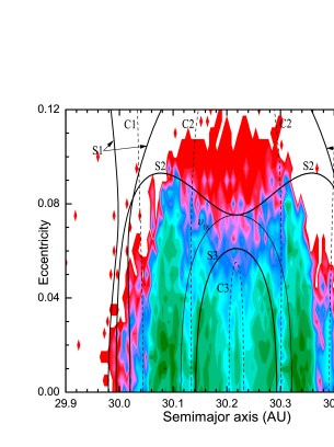
Figure 5: The locations of resonances plotted over the dynamical map for the case with initial inclination $i_{0}=5^{\circ}$. The C-type resonances are indicated by dashed curves while the solid curves stand for the S-type resonances, particularly, the secular resonance $\nu_{18}$ is plotted by the thin solid curve. See text to find the meaning of labels C1, C2, S1, S2 and S3.

The most distinguishable structure in the dynamical map of $i_{0}=5^{\circ}$ (and also other slices at low inclination, e.g. $i_{0}=0^{\circ},10^{\circ}$ in Fig. 3) is the blue vertical “stripes” indicating less stable motion. We find that they arise from the effects of some C-type resonances, among which three major ones are shown in Fig. 5. The dashed curves labeled by C1, C2 and C3 are locations of the following resonances:

$$\begin{array}[]{ll}{\rm C1}:&2f_{\sigma}-f_{2:1}+g_{6}=0,\\ {\rm C2}:&4f_{\sigma}-2f_{2:1}+g_{6}+g_{7}=0,\\ {\rm C3}:&6f_{\sigma}-3f_{2:1}+g_{5}+g_{6}+g_{7}=0.\end{array}$$ (6)

Apparently, their locations match the positions of vertical structures very well. We need to stress here that each resonance listed above (and below too) is just a representative of a bunch of resonances, characterized by higher order combinations of integers $p,q,p_{j},q_{j}$ in Eq. (5). For example, beside the resonance C1 that reaches the abscissa at $a_{0}=30.044$ au and $30.392$ au, we can easily find another two resonances as ${\rm C1^{\prime}:}\,2f_{\sigma}-f_{2:1}-g+g_{8}+g_{6}=0$ and ${\rm C1^{\prime\prime}:}\,2f_{\sigma}-f_{2:1}+g-g_{8}+g_{6}=0$. And in fact, the resonance C1 itself is favourable for the stability of Trojan orbit. As we will see in next Section, the asteroid 2001 QR322 is deep inside such a resonance and its orbit is stable over the Solar system age. On the contrary, the resonances ${\rm C1^{\prime}}$ and ${\rm C1^{\prime\prime}}$ are responsible for the unstable gaps in both sides of resonance C1, especially the apparent ones around $a_{0}=30.050$ au and $30.375$ au approximately.

Another mechanism that may contribute to the formation of the vertical structures is the secular nodal resonance $\nu_{18}$ defined by $s-s_{8}=0$. Its location is also plotted in Fig. 5, as well as other three S-type resonances:

$$\begin{array}[]{ll}{\rm S1}:&3g-g_{7}-g_{8}=0,\\ {\rm S2}:&g-2s+g_{8}-2s_{8}+2s_{5}=0,\\ {\rm S3}:&3s-2g_{8}-s_{8}=0.\end{array}$$ (7)

We notice inconsistent statements about the resonance $\nu_{18}$ in the literatures. Nesvorný and Jones [Nesvorný & Dones 2002] found in the dynamical map a less stable region with libration amplitude between $40^{\circ}$ and $50^{\circ}$ (Fig. 2(d) therein), and they argued that this arose from the effects of the $\nu_{18}$ resonance. While Brasser et al. [Brasser et al. 2004] showed that the clones of asteroid 2001 QR322 “remained deep inside” the $\nu_{18}$ resonance are the most stable ones (“have the longest e-folding time”). Marzari and Scholl [Marzari, Tricarico & Scholl 2003a] argued that this secular resonance were “not strong enough to cause a short term instability”. Our results support the same conclusion.

In Fig. 5, no apparent details in the dynamical map can be found around the location of $\nu_{18}$ resonance. In fact, we found in our simulations that nearly all orbits with low inclination ($i_{0}\leq 5^{\circ}$) and not too large libration amplitude are involved in the $\nu_{18}$ resonance, but this resonance does not show any prominent effects in protecting or destroying their orbital stabilities. The less stable region mentioned in Nesvorný and Jones [Nesvorný & Dones 2002] in fact corresponds to the blue stripes at $a_{0}=30.12$ au and $30.30$ au in the dynamical map of $i_{0}=0^{\circ}$ in Fig. 3, and it is clearly related to the C2 resonance in Eq. (6), but not the $\nu_{18}$ resonance.

Other secular resonances, e.g. the S1, S2 and S3 in Eq. (7), however may have more evident dynamical effects. The resonances S1 and S2 define the edge of the survival region, and the curvature of S2 in the eccentricity range of $0.07-0.09$ matches the outline of the stable region. The border between the stable region and chaotic region makes a V-shape blue area from $e_{0}=0.05$ to $e_{0}=0.09$, in which several crossovers or close encounters between resonances S2, S3, C2, C3 and $\nu_{18}$ happen. Thus it seems reasonable to argue that the border is made of a net of these resonances.

Another observing from Fig. 5 and other dynamical maps at different initial inclinations in Fig. 3 is that the C1-type resonance with $h=2,k=-1$ in Eq. (5) has quite promising dynamical effects in all initial inclination values, but the influences from C2 and C3 decreases as $i_{0}$ increases. The blue gaps corresponding to C2 and C3 become more and more vague as $i_{0}$ gets bigger. We will see this trend clearly in next example of $i_{0}=35^{\circ}$.

4.3 For $i_{0}=35^{\circ}$

Similarly, setting $\delta=a_{0}-30.220$, we obtain the best fits of the proper frequencies formulae for the slice $i_{0}=35^{\circ}$:

$$f_{\sigma}[10^{-4}\,2\pi{\rm/yr}]=1.0109-1.5923\delta^{2}+0.45999e^{2}$$

$$\\ -2.1860\delta^{4}-29.100e^{4}-5.1370\delta^{2}e^{2},$$ (8)

$$g[10^{-7}\,2\pi{\rm/yr}]=8.3905-4.9257\delta^{2}-6.113e^{2}$$

$$\\ -241.09\delta^{4}-75.306e^{4}-347.56\delta^{2}e^{2},$$ (9)

$$s[10^{-7}\,2\pi{\rm/yr}]=2.8989+15.920\delta^{2}+7.1909e^{2}$$

$$\\ -62.502\delta^{4}+161.75e^{4}+368.27\delta^{2}e^{2}.$$ (10)

Then by carefully studying the dynamical spectra, we detect some resonances involved in the motion. Using the above formulae, we calculate their locations and plot them over the corresponding dynamical map in Fig. 6.

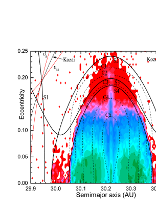
Figure 6: The same as Fig. 5 but for $i_{0}=35^{\circ}$. Except the resonances labeled by C1-C5 (dashed curves) and S1-S4 (solid curves. See text for their meanings), the locations of $\nu_{8},\nu_{18}$ resonances (solid curves in red) and Kozai resonance (thin solid curve in black) have also been plotted.

As in the previous case, we find in our calculations some C-type resonances involved in the motion of orbits with $i_{0}=35^{\circ}$, of which several typical ones are listed below and plotted in Fig. 6.

$$\begin{array}[]{ll}{\rm C1}:&2f_{\sigma}-f_{2:1}-g+2g_{6}=0,\\ {\rm C2}:&2f_{\sigma}-f_{2:1}-s+2s_{6}-s_{8}+g_{8}=0,\\ {\rm C3}:&2f_{\sigma}-f_{2:1}+g+2g_{6}-2g_{5}=0,\\ {\rm C4}:&2f_{\sigma}-f_{2:1}+2g+2g_{6}-3g_{5}=0,\\ {\rm C5}:&4f_{\sigma}-2f_{2:1}+3g_{6}+g_{5}-2g_{8}=0.\end{array}$$ (11)

The low-order C-type resonance like the C1 defined in Eq. (6) does not appear in the region around $i_{0}=35^{\circ}$. Among the resonances in Eq. (11), only the one with the lowest order (C1) has the distinguishable dynamical effects, shaping the sharp edge of stable region at low eccentricity ($e_{0}\leq 0.05$). The C-type resonance with $h=4,k=-2$ in Eq. (5), here C5 in Eq. (11) contributes to the formation of the vertical structure at the center (around $a_{0}=30.22$ au). Another interesting resonance is C2, in which the nodal precessions ($s,s_{8}$ and $s_{6}$) are involved. In fact, as the inclination of Trojan orbit increases, it is natural to expect that the nodal precession is becoming more important. We would like to note that there are less regular indentations corresponding to this resonance in the dynamical map at $a_{0}=30.08,30.36$ au and $e_{0}\geq 0.015$. On the other hand, although the resonances C3, C4 in Eq. (11) can be detected in the dynamical spectra, no apparent details in the dynamical map can be found related to these resonances.

The influences from the C-type resonances are less important in slice $i_{0}=35^{\circ}$ than in slice $i_{0}=5^{\circ}$. Relatively, the effects from the S-type resonances are remarkable. Beside the $\nu_{8},\nu_{18}$ and Kozai resonances that locate outside the survival region as show in Fig. 6, several other S-type resonances as below are determined and illustrated.

$$\begin{array}[]{ll}{\rm S1}:&g+s-g_{8}-s_{8}=0,\\ {\rm S2}:&g-2s+g_{8}-s_{8}+s_{5}=0,\\ {\rm S3}:&g+2s-g_{6}+s_{6}-3s_{5}=0,\\ {\rm S4}:&g-2s+g_{8}+s_{8}+g_{7}-g_{5}-s_{5}=0.\end{array}$$ (12)

Clearly the S2 resonance combined with S3 defines the boundary of the survival region, and the resonance S4 establishes the edge of the stable region up to $e_{0}=0.12$. Again, on the top part of the dynamical map, the C-type and S-type resonances gather, resulting in overlaps among them and leading to chaotic motion.

4.4 For $i_{0}=55^{\circ}$

Setting $\delta=a_{0}-30.223$, the formulae of the proper frequencies for the slice $i_{0}=55^{\circ}$ are:

$$f_{\sigma}[10^{-4}\,2\pi{\rm/yr}]=0.88663-1.1998\delta^{2}-2.0233e^{2}$$

$$\\ -7.4512\delta^{4}+353.60e^{4}-106.00\delta^{2}e^{2},$$ (13)

$$g[10^{-7}\,2\pi{\rm/yr}]=2.7724-46.683\delta^{2}-71.157e^{2}$$

$$\\ -1588.8\delta^{4}+666.87e^{4}-3776.5\delta^{2}e^{2},$$ (14)

$$s[10^{-7}\,2\pi{\rm/yr}]=1.5643-46.165\delta^{2}-52.989e^{2}$$

$$\\ +2168.4\delta^{4}+5116.5e^{4}+18800\delta^{2}e^{2}.$$ (15)

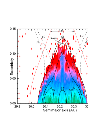
Figure 7: The same as Fig. 5 but for $i_{0}=55^{\circ}$. Except the resonances labeled by C1, C2 (dashed) and S1-S3 (solid. See text for the meanings), the locations of $\nu_{18}$ resonances (red lines) and Kozai resonance (thin solid curve in black) have also been plotted.

The involved important resonances are determined and illustrated in Fig. 7, where the following C-type and S-type resonances are plotted:

$$\begin{array}[]{ll}{\rm C1}:&2f_{\sigma}-f_{2:1}-2g+3g_{6}=0,\\ {\rm C2}:&2f_{\sigma}-f_{2:1}-g-s+3s_{6}=0,\\ {\rm S1}:&2s-2g_{5}-2s_{5}+g_{6}-s_{6}+g_{7}+s_{7}=0,\\ {\rm S2}:&s-2g_{7}+2s_{7}-s_{5}=0,\\ {\rm S3}:&s-g_{8}-s_{8}-g_{7}+g_{5}+s_{5}=0.\end{array}$$ (16)

Although the most part of the C1 lines in Fig. 7 are out of the survival region, we see the fine structures (narrow unstable gaps) around $a_{0}=30.06,30.36$ au and $e_{0}>0.002$ are clearly related to this resonance. Inversely, the stability of orbits benefits from the C2 resonance, as we see the concentration of stable orbits around the C2 lines, especially in the regions $a_{0}=30.13,30.31$ au and $e_{0}<0.002$.

Comparatively, the dynamical effects from S-type resonances are more prominent. As shown in Fig. 7, the S1 resonance sharply defines the out edge of the survival region; the lines of S2 coincide with the boundary separating the chaotic orbits from the relatively regular ones; and the S3 curves surround the most stable orbits in this slice.

Considering the high inclination of this slice at $i_{0}=55^{\circ}$, it is not a surprise to see that the nodal precession $s$ is involved more deeply in these important resonances compared to the low inclination cases (e.g., resonances listed in Eqs. (6), (7), (11) & (12)).

Meanwhile, the $\nu_{18}$ resonance (red lines) and Kozai resonance (thin black line) are calculated and shown in Fig. 7. The $\nu_{18}$ is outside the survival region, that is, it does not play an important role in the long-term stability of orbits. If an orbit was trapped in Kozai resonance, its inclination $i$ and eccentricity $e$ may experience joint variations: $i$ decreases as $e$ increases, or vice versa [Kozai 1962]. This variation may lead to a highly eccentric orbit and result in orbit escaping. Therefore, the boundary between the surviving and escaping orbits is determined cooperatively by the S1 and Kozai resonances.

4.5 A summary

At different inclinations, different resonances participate in featuring the dynamical maps. Basically, the secondary resonances (C-type) related to the libration of the 1:1 MMR between Neptune and its Trojans and to the quasi 2:1 MMR between Neptune and Uranus, as well as the secular resonances (S-type) related to the nodal and/or apsidal processions, are the most important dynamical mechanisms that form the fine details in the dynamical maps and determine the complicated orbital behavior of NTs. Compared to the cases in low inclination, those highly inclined orbits are more deeply affected by the nodal-type resonances. In all cases, different resonances with different orders make a resonance net in the parameter plane of initial conditions. Thus an orbit may diffuse slowly along the net and migrate on the parameter space from one configuration to another. Of particular interest is the slow diffusion from low inclination orbits to high inclination orbits, which can be used to explain the origins of the observed NTs with high-inclinations, i.e. 2005 TN53 and 2007 VL305 as listed in Table 1.

We only reported in previous subsections some resonances detected by the dynamical spectrum method. Surely, many more resonances, particularly those with high orders, have not been revealed in our current paper, and they may also play important roles in characterizing the dynamical behaviours of Trojans’ orbits, which are our studying topic in future.

5 Orbits of Observed Neptune Trojans

Up to now, six NTs have been observed, and their orbital stabilities have been analyzed individually, e.g. in [Marzari, Tricarico & Scholl 2003a, Brasser et al. 2004, Li, Zhou & Sun 2007]. Since we have presented global view of the dynamics of NTs, we can locate the observed NTs on the corresponding dynamical maps and draw conclusions directly from the comparison.

We have adopted the configuration of the outer solar system at epoch of August 1, 1993 (JD2449200.5) as the initial conditions to simulate the orbital evolutions of four planets and artificial Trojans, the dynamical maps (Fig. 3 in this paper and also Figs. 2 & 3 in Paper I) are based on the instantaneous orbital elements at that moment. But the orbits of observed NTs are given in recent epoch, e.g. the ones listed in Table 1 obtained from the AstDyS website are given at epoch JD2455000.5. To locate their orbits on the dynamical maps, we need to transfer their orbital elements at this moment to the epoch when the planets’ orbits are adopted. The transferred orbits are calculated and listed in Table 1.

Table 1: Orbits of observed Neptune’s Trojans at epochs JD=2455000.5 (June 14, 2009, six columns in the left half) and JD=2449200.5 (August 1, 1993, six columns in the right half) in the reference frame of J2000.0. The mean anomaly $M$, perihelion argument $\omega$, ascending node $\Omega$ and inclination $i$ are in degrees. All the angle values have been rounded to one decimal place for simplicity. The last column $\Delta\sigma$ gives the approximations of the libration amplitude (in degrees) of $\sigma$, derived from Fig. 2 in Paper I.

Designation	$M$	$\omega$	$\Omega$	$i$	$e$	$a$ (AU)	$\rightarrow$	$M$	$\omega$	$\Omega$	$i$	$e$	$a$ (AU)	$\Delta\sigma$
2001 QR322	57.31	162.5	151.6	1.3	0.0316	30.336	$\rightarrow$	30.06	155.3	151.6	1.3	0.0290	30.208	77
2004 UP10	343.40	357.5	34.8	1.4	0.0295	30.250	$\rightarrow$	303.65	2.8	34.7	1.4	0.0259	30.121	48
2005 TN53	289.14	84.8	9.3	25.0	0.0652	30.213	$\rightarrow$	250.71	88.7	9.3	25.1	0.0652	30.099	33
2005 TO74	270.02	301.7	169.4	5.2	0.0501	30.222	$\rightarrow$	230.28	306.9	169.4	5.2	0.0517	30.095	37
2006 RJ103	242.91	24.2	120.8	8.2	0.0276	30.112	$\rightarrow$	202.77	29.5	120.9	8.2	0.0318	29.990	22
2007 VL305	354.05	215.3	188.6	28.1	0.0648	30.081	$\rightarrow$	317.23	217.5	188.6	28.2	0.0620	29.982	20

Because all the six objects are on nearly circular orbits with eccentricities smaller than 0.07, we can approximately locate these orbits on the $(a_{0},i_{0})-$ plane in Paper I (Figs. 2 & 3) which are made for artificial Trojans with initial eccentricity $e_{0}\sim 0$. Since they are all around the leading Lagrange point ($L_{4}$), we should put them on Fig. 2 in Paper I (for $L_{4}$) to compare. A comparison tell clearly that five of them are inside the most stable regions (Regions A and B) and the only exception is 2001 QR322 (hereafter QR322 for short), whose position in the dynamical map is near the low-inclination end of the “arc structure”. We have shown in Paper I that this arc structure is related to a resonance as $f_{2:1}-2f_{\sigma}=g_{6}$, i.e., C1 in Eq. (6) of this paper.

A more accurate comparison can be performed by using the dynamical maps at different inclinations in this paper (e.g. Fig. 3). Recalling that all dynamical maps in this paper are for orbits around the trailing Lagrange point ($L_{5}$), we cannot put the observed orbits directly on the corresponding maps. Nevertheless, since the absolute symmetry between $L_{4}$ and $L_{5}$ have been proven [Nesvorný & Dones 2002, Marzari, Tricarico & Scholl 2003a, Zhou, Dvorak & Sun 2009a], it is possible to find the symmetrical counterpart around $L_{5}$ point for each orbit. To do so, we read from Fig. 2 in Paper I the libration amplitude $\Delta\sigma$ for each observed NT, which have been listed in the last column of Table 1. Then, remembering the inclination and neglecting the semimajor axis, the corresponding counterpart around $L_{5}$ is the one librating with the same $\Delta\sigma$ value on the $(a_{0},e_{0})-$ plane with the same inclination. For example, the object QR322 has a small inclination ($1.3^{\circ}$), and approximately we regard it as on the slice of $i_{0}=0^{\circ}$, i.e. the first panel in Fig. 3. We check the libration ($\Delta\sigma=77^{\circ}$) and find that the best counterpart of QR322 is $(a_{0},e_{0})\approx(30.38\,{\rm au},0.290)$. It is on the stable segment to the right of the unstable gap at $a_{0}\sim 30.375$ au. Similarly, we can locate the symmetrical correspondence of 2005 TO74 (hereafter TO74) in Fig. 5 for $i_{0}=5^{\circ}$ at $(a_{0},e_{0})\approx(30.26\,{\rm au},0.052)$. It is on the stable side of the boundary between stable and chaotic motion. Moreover, it’s in the very vicinity of the S3 resonance curve. We may conclude that the orbits of both QR322 and TO74 are stable and these objects, however, are probably influenced by resonances like C1 in Eq. (6) and S3 in Eq. (7), respectively. The rest four objects listed in Table 1, again this time, are well inside the most stable regions. Thus we neglect here the comparisons in detail.

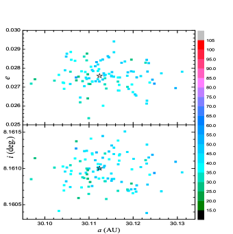
Figure 8: The orbital stabilities of 100 clones of 2006 RJ103. The color indicates the spectral number that is used as the stability indicator. The black stars designate the nominal orbital elements on the $(a,e)$ and $(a,i)$ plane (upper and lower panel respectively).

However, the observed orbits are not exactly on the slices we have calculated. To confirm our conclusion and to get more accurate estimation of the orbital stabilities, we integrate one hundred clones of each nominal orbit (note the numbers listed in Table 1 have been rounded for simplicity) and check their stabilities using the frequency analysis method adopted in our papers. Considering the uncertainties from observation and orbital determination, the clone orbits are generated using the covariance matrix given in the AstDyS webpage. We thank Dr. Antonio Giorgilli for supplying us the necessary computing codes for generating the proper initial conditions.

The results confirm the orbital stabilities of 2004 UP10, 2005 TN53, 2006 RJ103 and 2007 VL305. They are deeply inside the stable region, as proven by the fact that nearly all the clones of them have SN$<50$. As example, we present in Fig. 8 the SN of clones of 2006 RJ103. Out of the 100 orbits, only 4 have SN$>50$ with the largest SN$=57$.

As mentioned above, TO74 is close to the edge of stable region. Considerable fraction ($\sim 50\%$) of the clones has relatively large SN$\sim 70$. And there is a trend of declining SN as the eccentricity of clones decreases. Thus we may expect that further observations will constrain the eccentricity to a smaller value.

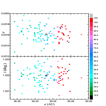
Figure 9: The same as Fig. 8, but for object 2001 QR322.

The most interesting result is from the case for QR322, as shown in Fig. 9. Because QR322 is in a narrow stable “stripe-like” area separated from the main stable region in the dynamical map, some clones of this object are protected by the C-type resonance $f_{2:1}-2f_{\sigma}=g_{6}$, while some other clones nearby may suffer the destroying effects from resonance like $2f_{\sigma}-f_{2:1}-g+g_{8}+g_{6}=0$ and its analogues. In Fig. 9, we see the stability of clones depends sensitively on the semimajor axis, which can be explained by the sensitive dependence of the libration frequency $f_{\sigma}$ on semimajor axis. The eccentricity and inclination within the observing error range, on the other hand, do not influence the orbital stability considerably. Similar results can also be found in [Horner & Lykawka 2010b], where the lifetime of clones has a sharp edge on semimajor axis (Figs. 3 & 4 therein). In this sense, the QR322 is not a typical (thus not a good) example of NTs. If using it as a seed to generate a cloud of artificial asteroids around to represent the real NTs [Horner & Lykawka 2010a], additional attention should be paid to make the conclusion drawn from the orbital simulations of the cloud consistent and convictive.

In addition, we have integrated the six nominal orbits up to the Solar system age (4.5 Gyr) and found that all of them survive on the Trojan-like orbits. According to our investigations above, it is an expectable outcome for five objects. But for QR322, we would like to say, it is more or less by luck. Not like others, only a very slight deviation from the nominal orbit of QR322 may lead to an unstable orbit.

Figure 10: The orbital evolution of a clone of 2001 QR322. From top to bottom, we illustrate in 8 panels the temporal evolution of $a,e,i,\omega$ (critical angle of Kozai resonance), $\Omega,\sigma=\lambda-\lambda_{8}$ (resonant angle of the 1:1 mean motion resonance), $\Delta\varpi=\varpi-\varpi_{8}$ (critical angle of $\nu_{8}$ resonance) and $\Delta\Omega=\Omega-\Omega_{8}$ ( critical angle of $\nu_{18}$ resonance).

In Fig. 10, we show such an example. The initial orbit is exactly the literal one listed in Table 1, in which the numbers have been rounded for simplicity, e.g. the inclination $1.3^{\circ}$ is rounded from the nominal value $1.3220^{\circ}$. At the beginning $1\times 10^{5}$ yrs, the orbit has a quite regular behaviour. The eccentricity is small, the inclination is constrained below $4^{c}irc$, and the resonant angle $\sigma$ varies with an amplitude smaller than $70^{\circ}$. In most of the time, it is trapped in the $\nu_{18}$ resonance, as $\Delta\Omega$ librates around $0^{\circ}$ with an amplitude smaller than $180^{\circ}$. Then from $1.05\times 10^{5}$ yrs, the eccentricity increases and the orbit loses stability, escaping from the Trojan-like orbit.

A close observation at Fig. 10 may reveal that as early as $4\times 10^{4}$ yrs, some chaotic features can be found in the semimajor axis’ behaviour, and the eccentricity begins to show a slow increasing trend from $8\times 10^{4}$ yrs. We think it is due to the fact that this orbit is in the resonance $2f_{\sigma}-f_{2:1}-g+g_{8}+g_{6}=0$. The libration $f_{\sigma}$ and apsidal precession $g$ are involved in this resonance, therefore the chaos was introduced to the behaviour of $a$ and $e$. Finally, the resonance results in totally chaotic orbit.

6 Conclusions

As a continuation of our research in a previous paper on the dynamics of NTs, we present in this paper a detailed investigation on the stability of orbits on the initial plane of $(a_{0},e_{0})$. By constructing dynamical maps on slices with different inclinations $i_{0}$, we obtain a global view of the stability of NTs in the whole orbital parameter space.

In the three most stable regions in inclination, we found in the representative dynamical maps the extension of stable motion in eccentricity is 0.10 for low-inclination orbits with $i_{0}<12^{\circ}$, 0.12 for medium inclination $22^{\circ}<i_{0}<36^{\circ}$, and 0.04 for high inclination between $51^{\circ}$ and $59^{\circ}$. The feature of dynamical map was enriched by fine structures in it, indicating the diversity of orbital behaviour of NTs.

Using the dynamical spectrum method based on the frequency analysis, we figured out the mechanisms creating the fine structures in the dynamical maps. We found two types of resonance may involve deeply in the dynamics of NT. One is the secondary resonance (C-type) concerning mainly two frequencies: the libration frequency of the resonant angle $\sigma=\lambda-\lambda_{8}$ and the frequency of the quasi 2:1 MMR between Neptune and Uranus $2\lambda_{8}-\lambda_{7}$. The other is the secular resonance in general sense (S-type), characterized by the commeasurability between different combinations of secular frequencies, such as the frequencies of apsidal and/or nodal precessions of NT and/or planets. Among the well-known secular resonances, the $\nu_{8}$ resonance is very effective in driving a Trojan to highly eccentric orbit thus make a deep unstable gap in inclination around $44^{\circ}$. On the contrary, the $\nu_{18}$ resonance, found nearly everywhere at low inclination, is so weak that it has hardly any influence on the dynamics of NT.

Our study is not just theoretical, since we can place the observed NTs on the dynamical map and check whether they are trapped in or close to some identified resonances. In this way, the dynamical features of the observed objects can be predicted. We found 2004 UP10, 2005 TN53, 2006 RJ103 and 2007 VL305 are deeply inside the region of the most regular motion, far away from dominant destructive secular resonances. Therefore they must be stable. The orbits of 2001 QR322 and 2005 TO74 may survive to the Solar system age, but they are probably influenced by specific C-type and S-type resonances, respectively. And future observations may constrain their orbits to stable region a little deeper. To confirm the above conclusions, hundreds of orbital clones of the six observed objects were generated within the observational error bars, their orbits were integrated numerically, and their stabilities were carefully inspected.

Surely, the resonances listed in Eqs. (6), (7), (11), (12), (16) are not all of the possible resonances involved in the orbital evolution. Especially, we may miss some important resonances with higher order. However, even only these resonances listed in our paper, have built a “resonant net” that connect different parts of the whole orbital parameter space. Correspondingly, there must be such a net in the phase space. With the help of this net, an orbit may diffuse in the phase space, resulting in significant change in the orbital behaviour. Long-term diffusion may be expectable along the net. The most attractive diffusion, probably is the slow transferring of an orbit from low inclination to high inclination. Although in our preliminary tests, we did not find such inclination-increasing phenomenon, we would argue that this is a very important issue. The importance arises not only from the interesting dynamics itself, but also from the fact that this problem is closely related to the origins of those highly inclined NTs. Again, their origins are closely related to the evolution of our planetary system in the early stage [Kortenkamp, Malhotra & Michtchenko 2004, Nesvorný & Vokrouhlický 2009].

Another possible hint about the early evolution of the Solar system is buried in the C-type resonances. On one hand, C-type resonances are quite powerful in featuring the dynamics of NTs. On the other hand, these resonances are sensitively affected by the frequency $f_{2:1}$. If the planetary orbital configuration changed, even only very little, $f_{2:1}$ would change and this would lead to significant varying in the position and strength of the C-type resonances. Thus a careful discussion on the influences of the C-type resonances, under current planetary configuration and under other possible configuration, is critical. Similar analysis have been performed in the case of the formation of the Hecuba Gap in the main asteroid belt, where the Great Inequality (quasi 5:2 MMR between Jupiter and Saturn) plays the role of $f_{2:1}$ here [Henrard 1997]. A closer analogue is about Jupiter Trojans [Robutel & Bodossian 2009]. For NTs, some work have been done [Nesvorný & Vokrouhlický 2009, Lykawka et al 2010], and our contribution is also undergoing.

References

- [Brasser et al. 2004] Brasser R., Mikkola S., Huang T.-Y., Wieggert P., Innanen K., 2004, MNRAS, 347, 833
- [Dvorak et al. 2007] Dvorak R., Schwarz R., Süli Á., Kotoulas T., 2007, MNRAS, 382, 1324
- [Dvorak, Bazso & Zhou 2010] Dvorak R., Bazso A., Zhou L.-Y., 2010, Celest. Mech. & Dyn. Astr., 107, 51
- [Érdi 1988] Érdi B., 1988, Celest. Mech., 43, 303
- [Ferraz-Mello et al. 2005] Ferraz-Mello S., Michtchenko T.A, Beaugé C., Callegari Jr. N., 2005, in Dvorak R., Freistetter R., Kurths J., eds. Chaos and Stability in Extrasolar Planetary Systems, Lecture Notes in Physics, Springer, p.219
- [Hanslmeier & Dvorak 1984] Hanslmeier A., Dvorak R., 1984, A&A, 132, 203
- [Henrard 1997] Henrard J., 1997, Celest. Mech. & Dyn. Astr., 69, 187
- [Horner & Lykawka 2010a] Horner J., Lykawka P.S., 2010a, MNRAS, 402, 13
- [Horner & Lykawka 2010b] Horner J., Lykawka P.S., 2010b, MNRAS, 405, 49
- [Kortenkamp, Malhotra & Michtchenko 2004] Kortenkamp S., Malhotra R., Michtchenko T., 2004, Icarus, 167, 347
- [Kozai 1962] Kozai Y., 1962, AJ, 67, 591
- [Li, Zhou & Sun 2007] Li J., Zhou L.-Y., Sun Y.-S., 2007, A&A, 464, 775
- [Lykawka et al 2009] Lykawka P., Horner J., Jones B., Mukai T., 2009, MNRAS, 398, 1715
- [Lykawka et al 2010] Lykawka P., Horner J., Jones B., Mukai T., 2010, MNRAS, 404, 1272
- [Marzari, Tricarico & Scholl 2003a] Marzari F., Tricarico P., Scholl H., 2003a, A&A, 410,725
- [Marzari, Tricarico & Scholl 2003b] Marzari F., Tricarico P., Scholl H., 2003b, MNRAS, 345, 1091
- [Michtchenko & Ferraz-Mello 1995] Michtchenko T., Ferraz-Mello S., 1995, A&A, 303, 945
- [Michtchenko et al. 2002] Michtchenko T., Lazzaro D., Ferraz-Mello S., Roig F., 2002, Icarus, 158, 343
- [Milani 1993] Milani A., 1993, Celest. Mech. & Dyn. Astr., 57, 59
- [Milani 1994] Milani A., 1994, in Milani A., Martino M., Cellino A., eds, Proc. IAU Symp. 160, Asteroids, Comets, Meteors 1993. Kluwer Academic Publisher, Netherlands, p.159
- [Murray & Dermott 1999] Murray C.D., Dermott S.F., 1999, Solar System Dynamics, Cambridge Univ. Press, Cambridge
- [Nesvorný & Dones 2002] Nesvorný D., Dones L., 2002, Icarus, 160, 271
- [Nesvorný et al. 2002] Nesvorný D., Thomas F., Ferraz-Mello S., Morbidelli A., 2002, Celest. Mech. & Dyn. Astr., 82, 323
- [Nesvorný & Vokrouhlický 2009] Nesvorný D., Vokrouhlický D., 2009, AJ, 137, 5003
- [Nicholson 1961] Nicholson S., 1961, Astron. Soc. Pac. Leaf., 8, 239
- [Robutel & Gabern 2006] Robutel P., Gabern F., 2006, MNRAS, 372, 1463
- [Robutel & Bodossian 2009] Robutel P., Bodossian J., 2009, MNRAS, 399, 69
- [Sheppard & Trujillo 2006] Sheppard S., Trujillo C., 2006, Sci, 313, 511
- [Zhou, Dvorak & Sun 2009a] Zhou L.-Y., Dvorak R., Sun Y.-S., 2009a, MNRAS, 398, 1217
- [Zhou, Dvorak & Sun 2009b] Zhou L.-Y., Dvorak R., Sun Y.-S., 2009b, in Zhang S., Li Y., Yu Q. eds, Proceedings of the 10th APRIM, 91, 2009