Entanglement entropy of integer Quantum Hall states in polygonal domains

Abstract

The entanglement entropy of the integer Quantum Hall states satisfies the area law for smooth domains with a vanishing topological term. In this paper we consider polygonal domains for which the area law acquires a constant term that only depends on the angles of the vertices and we give a general expression for it. We study also the dependence of the entanglement spectrum on the geometry and give it a simple physical interpretation.

I Introduction

The area law satisfied by the entanglement entropy of the low energy states of quantum many body systems in Condensed Matter and Field Theory, has become one of the most fundamental tools to study the physical properties of these complex systems amico ; cirac ; plenio . To define this entropy one considers a low energy state $\psi$, usually the ground state, and computes the reduced density matrix $\rho_{A}$ by tracing out the degrees of freedom outside a domain $A$. The entanglement entropy $S_{A}(\psi)$, associated to the state $\psi$ and the domain $A$, is defined as the von Neumann entropy of the reduced density matrix $\rho_{A}$, i.e. $S_{A}(\psi)=-{\rm tr}\rho_{A}\log\rho_{A}$. The area law states that $S_{A}(\psi)$ is proportional to the size of the boundary of $A$. In 3D this size is the area separating $A$ from its environment, which gives the law its name. In lower dimensions one should rather used the terms perimeter law in 2D and zeroth law in 1D, but those names are not customary.

Three issues are important regarding the area law: violations, fluctuations and subleading corrections. They all provide a great amount of information about the system. In conformal invariant 1D models, the area law shows a log violation proportional to the central charge of the corresponding CFT and the topology open/close of the system log ; latorre ; korepin ; cardy . Fluctuations around the log law for the Renyi entropy in Luttinger liquids allows a determination of the Luttinger parameter cala-par , and subleading terms contain information about the scaling dimensions of the operators cala-corre .

In 2D much less is known about corrections to the area law. In systems with topological order, the correction is a constant term $\gamma$ denoted topological entanglement entropy kitaev ; levin , and whose value is given by the logarithm of the total quantum dimension of the anyonic excitations. The area law of the Fractional Quantum Hall (FQH) states has been the target of several recent studies schoutens1 ; schoutens2 ; laeuchli ; friedman ; fradkin , in order to confirm its validity and to compute the value of $\gamma$ predicted in kitaev ; levin . Reference fradkin uses Chern-Simons theory, finding the predicted value of $\gamma$, however the linear behaviour of $S_{A}$, is not captured, due to the purely topological nature of this theory. There are numerical studies using the Laughlin wave function schoutens1 ; schoutens2 ; laeuchli and exact diagonalization friedman ; laeuchli , for filling fractions $\nu=1/3,1/5$ and the $\nu=5/2$ Pfaffian state. The approaches of schoutens1 ; schoutens2 ; laeuchli ; friedman use the orbital basis for the Landau levels. The close relationship of this basis to the spatial partioning of the blocks leads to an area law of the form $S_{A}=c\sqrt{l_{A}}-\gamma+O(1/l_{A})$, where $l_{A}$ is the number of Landau orbitals in the block $A$. The numerical values of $\gamma$ computed in the spherical geometry schoutens1 and the torus geometry friedman ; laeuchli agree, within some precision, with their theoretical values, despite of the fact that the systems analyzed are not very large.

For non topological models there are also some results. In those with a Fermi surface, the area law exhibits a log violation fermi1 ; fermi2 ; fermi3 ; fermi4 ; fermi5 ; fermi6 reminiscent of the 1D conformal systems, which suggest that higher dimensional bosonization methods may give an appropiate description hal-boso . Corrections to the area law in non-smooth domains, in $2+1$ dimensions, have been obtained in relativistics free bosons and fermions in ref.CH and in an interacting CFT using the Ads/CFT conjecture in Ads . The 2D quantum critical models of Fradkin and Moore FradMoore with critical exponent $z=2$ have also universal subleading contributions (see also fra1 ).

The aim of this paper is to calculate the entanglement entropy of the IQHE ground state in arbitrary polygonal domains. We obtain that the entanglement entropy is given by the area (or perimeter) law plus a contribution due to the vertices, $\gamma$, that only depends on the angle of the vertices and the density of the fluid of electrons.

In the following we shall concentrate in the IQHE state with filling fraction $\nu=1$ defined on a cylindrical geometry, but the calculation of $\gamma$ for higher filling fractions and different geometries are easily generalizable.

Let us consider the Landau model for a particle in a cylinder of size $L_{x}\times L_{y}$. The one particle wave function in the lowest Landau level (LLL), in the gauge ${\bf A}=B(0,x)$, is (in units of the magnetic length $\ell$ equal to one):

$$\phi_{k_{y}}(x,y)=\frac{1}{\pi^{1/4}L_{y}^{1/2}}\;e^{ik_{y}y}\;e^{-(x-k_{y})^{2}/2}.$$ (1)

On the cylinder, the identification of the wave function along the $y$ direction implies:

$$k_{y}=\frac{2\pi n}{L_{y}},\quad-\frac{n_{0}}{2}+1\leq n\leq\frac{n_{0}}{2}.$$ (2)

The number of LLLs, $n_{0}$, is obtained imposing that the particle lives in the strip $|x|\leq L_{x}/2$, which yields $n_{0}=\frac{L_{x}L_{y}}{2\pi}$. This value also gives the total number of quantum fluxes through the box. The electron operator can be written as

$$\psi(x,y)=\sum_{k_{y}}\phi_{k_{y}}(x,y)c_{k_{y}}+{\rm higher}\;{\rm LLs},$$ (3)

where $c_{k_{y}}$ is the fermionic destruction operator of the LLL labeled by $k_{y}$. The extra term in (3) involves the remaining Landau levels, which are empty for filling fraction $\nu=1$. The ground state for $\nu=1$ is given by:

$$|\Phi_{0}\rangle=\Pi_{k_{y}}c_{k_{y}}^{\dagger}|0\rangle,$$ (4)

where $|0\rangle$ is the Fock vacuum. The two point fermion correlator in this state is,

$$C_{\textbf{r},\textbf{r'}}=\langle\Phi_{0}|\psi^{\dagger}(x,y)\;\psi(x^{\prime},y^{\prime})|\Phi_{0}\rangle.$$ (5)

Using (3) and (4) one finds:

$$C_{\textbf{r},\textbf{r'}}=\sum_{k_{y}}\phi_{k_{y}}^{*}(x,y)\;\phi_{k_{y}}(x^{\prime},y^{\prime}).$$ (6)

We want to compute the entanglement entropy, $S_{\mathcal{D}}$, of the state $\Phi_{0}$, in a polygonal domain $\mathcal{D}$ embedded in a cylinder of radius $L_{y}$ such as that shown in fig.1.

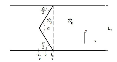
Figure 1: Domain $\mathcal{D}=\mathcal{D}_{A}\cup\mathcal{D}_{B}$ including two vertices with angle $\alpha$. Varying the parameter $l_{x}=\frac{LCot(\alpha/2)}{2}$ we can obtain the correction to the area law, $\gamma$, for $\alpha\in[0,\pi]$.

This entropy is given by the formula $S_{\mathcal{D}}=-{\rm tr}\,\rho_{\mathcal{D}}\log\rho_{\mathcal{D}}$ where $\rho_{\mathcal{D}}={\rm tr}_{\mathcal{D}_{c}}|\Phi_{0}\rangle\langle\Phi_{0}|$, and $\mathcal{D}_{c}$ is the complement of $\mathcal{D}$ in the cylinder. The computation of $S_{\mathcal{D}}$ is done in two steps latorre ; peschel . First one restricts the correlation matrix $C_{\textbf{r},\textbf{r'}}$, to the domain $\mathcal{D}$, i.e.

$$\tilde{C}_{\textbf{r},\textbf{r'}}=C_{\textbf{r},\textbf{r'}},\quad\textbf{r},\textbf{r'}\in\mathcal{D}.$$ (7)

Next, one diagonalizes $\tilde{C}_{\textbf{r},\textbf{r'}}$, i.e.

$$\int_{\mathcal{D}}d^{2}\textbf{r'}\;\tilde{C}_{\textbf{r},\textbf{r'}}\;g(\textbf{r'})=\lambda g(\textbf{r}).$$ (8)

The entropy $S_{\mathcal{D}}$ is obtained by means of,

$$S_{\mathcal{D}}=\sum_{m}H(\lambda_{m}),$$ (9)

where $H(x)=-x\log x-(1-x)\log(1-x)$. We have introduced a parameter $l_{x}$ that allow us to vary the angle $\alpha$ (see fig.1). If $l_{x}=0$, the domain $\mathcal{D}(l_{x}=0)=\mathcal{D}_{0}$ becomes a half cylinder. The eigenvalues of the correlator (7) for this case were given in we :

$$\lambda_{n}=\int_{\mathcal{D}_{0}}\phi^{*}_{n}(x,y)\phi_{n}(x,y)dxdy=\frac{1}{2}\left(1-Erf\left(\frac{2n\pi}{L_{y}}\right)\right),$$

$$n=-\infty,..,\infty\ .$$ (10)

In this formula we assumed that $L_{x}$ is effectively infinite. Computing now the entanglement entropy (9) using (10) one obtains $S_{\mathcal{D}_{0}}=0.203291*L_{y}$. Observe that $L_{y}$ coincides with the perimeter of $\mathcal{D}_{0}$, but this is a general result that holds for any smooth domain $\mathcal{D}_{smooth}$, i.e.:

$$S_{\mathcal{D}_{smooth}}=c*P,$$ (11)

where $P$ is the perimeter of $\mathcal{D}_{smooth}$ and the constant

$$c=0.203291$$ (12)

is independent of the geometry of the system but varies with the number of fully occupied Landau levels we .

II Correction to the area law

The aim of this section is to show that the area law for a polygonal domain $\mathcal{D}$ is given by

$$S_{\mathcal{D}}=S_{\mathcal{D}_{smooth}}+\gamma,$$ (13)

where $S_{\mathcal{D}_{smooth}}$ is the entanglement entropy of a smooth domain $\mathcal{D}_{smooth}$ with the same perimeter as $\mathcal{D}$, given by eq. (11), and $\gamma$ is a constant term due to the corners of the domain.

To proof eq.(13) we start by diagonalizing the correlator (7) in a generic domain $\mathcal{D}$. Using (1) and (6) equation (8) can be written as:

$$\sum_{n}\phi_{n}^{*}(x,y)\int_{D}\phi_{n}(x^{\prime},y^{\prime})g(x^{\prime},y^{\prime})=\sum_{n}\phi_{n}^{*}(x,y)A_{n}$$ (14)

$$= \lambda g(x,y)\ ,$$

where we have defined:

$$A_{n}=\int_{\mathcal{D}}dx^{\prime}dy^{\prime}\phi_{n}(x^{\prime},y^{\prime})g(x^{\prime},y^{\prime})\ .$$ (15)

The vanishing eigenvalues $\lambda$ of equation (8), does not contribute to $S_{\mathcal{D}}$, so one can focus on the non vanishing ones. Using equation (14), the corresponding eigenfunctions $g(x,y)$, can be written as

$$g(x,y)=\frac{1}{\lambda}\sum_{m}\phi_{m}^{*}(x,y)A_{m}.$$ (16)

Finally, replacing (16) into (15) one obtains the following equation for the eigenvalues:

$$\sum_{m}\left(F_{\mathcal{D}}\right)_{nm}A_{m}=\lambda A_{n}\ ,$$ (17)

where $F_{\mathcal{D}}$ is a matrix with elements

$$\left(F_{\mathcal{D}}\right)_{nm}=\int_{\mathcal{D}}\phi_{n}(x,y)\phi_{m}^{*}(x,y).$$ (18)

Observe that the continuous eigenvalue equation (8) has been converted into a discrete one (17), where the eigenvalues of the matrix $F_{\mathcal{D}}$ are those of the correlator (7). This fact will allow us to apply numerical methods to find the eigenvalues $\lambda$.

Indeed, let us first show the validity of equation (13) for some simple domains as those depicted in fig.2. The domains $\mathcal{D}_{n}$, with $n=4,6,8,10$, are four different polygons with $n$ right angles.

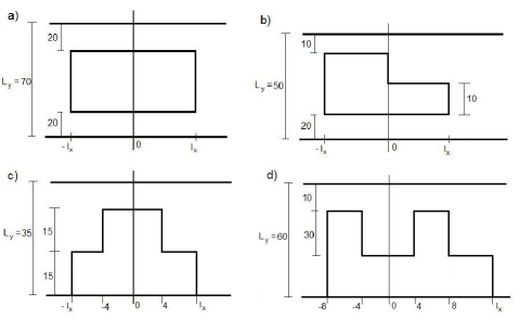
Figure 2: Different domains in the torus with 4,6,8 and 10 right angles.

For each of these domains we first compute the matrix $F_{\mathcal{D}}$ (see 18), and we diagonalize it for different values of $P$. The corresponding entropies $S_{\mathcal{D}_{n}}$ can be fitted to the formulas:

a) $S_{\mathcal{D}_{4}}=-0.341315+0.203291*P_{\mathcal{D}_{4}}$,
b) $S_{\mathcal{D}_{6}}=-0.512909+0.203295*P_{\mathcal{D}_{6}}$,
c) $S_{\mathcal{D}_{8}}=-0.683902+0.203291*P_{\mathcal{D}_{8}}$,
d) $S_{\mathcal{D}_{10}}=-0.85412+0.203289*P_{\mathcal{D}_{10}}$.

Notice that the constant multiplying the perimeters $P_{\mathcal{D}_{n}}$ agrees, to great accuracy, with the value $c$ in (11) for smooth domains. From these examples one can extract the value of $\gamma$ for right angles:

$$\gamma\left(\frac{\pi}{2}\right)=a\left(\frac{\pi}{2}\right)*(\mbox{number of }\pi/2\mbox{ vertices})\ ,$$ (19)

with $a\left(\frac{\pi}{2}\right)=-0.0855$. Based on (13,19) we can propose a general expression for the entanglement entropy of an arbitrary domain $\mathcal{D}$ with $n$ vertices parameterized by angles $\alpha_{i}\;(i=1,\dots,n)$

$$S_{\mathcal{D}} = S_{\mathcal{D}_{smooth}}+\gamma,\qquad\mbox{with}$$

$$\gamma(\{\alpha_{i}\}) = \sum_{i}a(\alpha_{i})*n_{i}\ ,\quad\alpha_{i}\in[0,2\pi],$$

with $n_{i}$ the number of vertices with angle $\alpha_{i}$ in the boundary of $\mathcal{D}$. Each of these angles varies between 0 and $2\pi$, but as we show below, the parameter $\gamma$ is invariant under the symmetry $\alpha\leftrightarrow 2\pi-\alpha$, which follows from the equality of the entropy of a pure state in a domain and its complement. For this reason we can restrict $\alpha$ to the interval $\mbox{[}0,\pi\mbox{]}$.

The calculation of $a(\alpha)$ can be done considering the domain of fig.1. For different values of $\alpha\in\mbox{[}0,\pi\mbox{]}$ (or $l_{x}$ in fig.1), we diagonalize the $F_{\mathcal{D}}$ matrix, calculate $S_{\mathcal{D}}$ and finally using (LABEL:generalgam), we obtain the value of $a(\alpha)$ by means of the equation

$$a(\alpha)=\frac{1}{2}\left(S_{\mathcal{D}}-0.20329*P_{\mathcal{D}}\right)\ ,$$ (21)

with $P_{\mathcal{D}}$ the perimeter of $\mathcal{D}$. The factor $\frac{1}{2}$ in (21) arises from the fact that the domain of fig.1 contains two vertices with angle $\alpha$. The numerical determination of $a(\alpha)$ is given in fig.3. This curve can be fitted with the following expansion in the variable $2l_{x}/L_{y}=\left|\cot(\alpha/2)\right|$ (see fig.1) :

$$a(\alpha)=0.00723706\left|\cot(\alpha/2)\right|-0.155709\left|\cot(\alpha/2)\right|^{2}+$$

$$0.0876488\left|\cot(\alpha/2)\right|^{3}-0.0306014\left|\cot(\alpha/2)\right|^{4}+$$

$$0.00698332\left|\cot(\alpha/2)\right|^{5}-0.00105786\left|\cot(\alpha/2)\right|^{6}+$$

$$0.000105322\left|\cot(\alpha/2)\right|^{7}-6.616*10^{-6}\left|\cot(\alpha/2)\right|^{8}+$$

$$2.375*10^{-7}\left|\cot(\alpha/2)\right|^{9}-3.7112*10^{-9}\left|\cot(\alpha/2)\right|^{10}.$$

(22)

Note that (22) satisfies the relation $a(\alpha)=a(2\pi-\alpha)$ that together with (LABEL:generalgam) imply that $S_{\mathcal{D}}=S_{\mathcal{D}_{c}}$ ($\mathcal{D}_{c}$ is the complement of $\mathcal{D}$) as explained above. Hence, we can restrict ourselves to the interval $\alpha\in\mbox{[}0,\pi\mbox{]}$ where $\cot(\alpha/2)\geq 0$ so that we can drop the absolute values in (22).

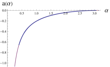
Figure 3: Plot of $a(\alpha)$ vs. $\alpha$ for $\alpha\in[0,\pi]$: the dotted line corresponds to the values of $a(\alpha)$ obtained by diagonalization of the $F_{\mathcal{D}}$ matrix (17) and the continuous line shows fit (22). There is a perfect matching between the two curves.

In order to assess the accuracy of the fit (22) we can compare the entanglement entropies obtained by diagonalization of the $F_{\mathcal{D}}$ matrix (17), for the complicated domains of fig.4, with the theoretical formula (LABEL:generalgam) using the extrapolation (22).

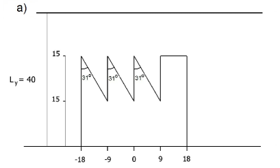
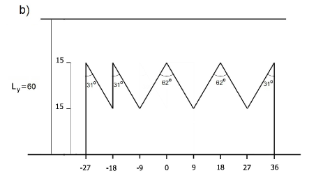
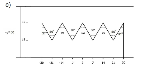
Figure 4: The domains a) b) and c) with perimeters P=202.479, 260.45 and 254.3033 respectively are used to check the validity of (LABEL:generalgam) and (22) .

In the case of diagonalization of the $F_{\mathcal{D}}$ matrix we obtain:

$$S_{a} = 38.04348652\ ,\quad S_{b}=50.02330873\quad\mbox{and}$$

$$S_{c} = 48.92750022\$$ (23)

and using (LABEL:generalgam) and (22) we arrive at

$$S_{a} = 0.20329*P+4*a(\pi/2)+6*a(\arctan(9/15))$$

$$= 38.047,$$

$$S_{b} = 0.20329*P+2*a(\pi/2)+4*a(\arctan(9/15))+$$

$$5*a(2*\arctan(9/15))=50.0253\qquad\mbox{and}$$

$$S_{c} = 0.20329*P+2*a(\pi/2)+2*a(\arctan(9/15))+$$ (24)

$$2*a(\arctan(7/15)+\arctan(9/15))+$$

$$5*a(2*\arctan(7/15))=48.927.$$

The comparison of (23) and (24) shows clearly the validity of (LABEL:generalgam) and of the extrapolation (22). The previous results have been obtained for a cylindrical geometry, however it can be shown that $a(\alpha)$ is the same function for the sphere and the plane and thus $\gamma$ is also independent of the geometry.

III Analytical calculation of $a(\alpha)$.

In this section we shall give an analytical justification of equation (LABEL:generalgam). A crucial point in our analysis is that the eigenvalue $\lambda_{n}(l_{x},L_{y})$ of the $F_{\mathcal{D}}$ matrix (17), corresponds to a deformation of the eigenvalue (10) for the case of the smooth domain $\mathcal{D}_{0}$ ($l_{x}=0$ in fig.1). This result can be shown by diagonalization of $F_{\mathcal{D}}$ for many different values of $l_{x}$ and $L_{y}$. This deformation is parameterized by a function $\kappa(l_{x},L_{y})$ and it is given by :

$$\lambda_{n}(l_{x},L_{y})=\frac{1}{2}\left(1-Erf\left[\frac{2n\pi}{L_{y}}\left(1-\kappa(l_{x},L_{y})\right)\right]\right).\$$

(25)

In fig.5 we show, for the particular case $l_{x}=21$ and $L_{y}=30$ ($\alpha=71.075^{\circ}$ in fig.5), the perfect matching between the eigenvalues obtained by diagonalization of the $F_{\mathcal{D}}$ matrix with those given by (25).

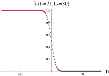
Figure 5: Overlap between the eigenvalues $\lambda_{n}(l_{x}=21,L_{y}=30)$ obtained by diagonalization of the $F_{\mathcal{D}}$ matrix (17) and those obtained using the deformation (25) with $\kappa(l_{x},L_{y})=0.40266$.

To calculate the function $\kappa(l_{x},L_{y})$ we can use equations (9),(LABEL:generalgam),(25) and the change of variables $x=(2\pi n/L_{y})\left(1-\kappa(l_{x},L_{y})\right)$ obtaining:

$$S_{\mathcal{D}}=cP_{\mathcal{D}}+2a(\alpha)=\int_{-\infty}^{\infty}H[\lambda_{n}(l_{x},L_{y})]dn$$ (26)

$$= \frac{L_{y}c}{(1-\kappa(l_{x},L_{y}))}\ ,$$

with $P_{\mathcal{D}}=2\sqrt{\left(\frac{L_{y}}{2}\right)^{2}+l_{x}^{2}}$ the perimeter of $\mathcal{D}$ and $c$ given in (12). From equation (26), the deformation $\kappa(l_{x},L_{y})$ is expressed by:

$$\kappa(l_{x},L_{y})=1-\frac{L_{y}c}{(cP_{\mathcal{D}}+2a(\alpha))},\$$ (27)

with $a(\alpha)$ given by the extrapolation (22) or by the theoretical value (32) to be obtained below.

Equation (25) is rather interesting since it shows that the whole spectrum of the matrix $F_{\mathcal{D}}$ is given in terms, basically, of the function $\kappa(l_{x},L_{y})$. Hence, we expect that overall quantities like $Tr\,F^{p}_{\mathcal{D}}=\sum_{n}\lambda_{n}^{p}(l_{x},L_{y})$, will also depend on the latter function. If for some $p$, we were able to compute this trace, then we will know $\kappa(l_{x},L_{y})$ as well $a(\alpha)$ by means of eq.(27). The simplest choice is $p=1$, but in this case the trace of $F_{\mathcal{D}}$ does not depend on $\kappa(l_{x},L_{y})$. This follows from the relations

$$TrF_{\mathcal{D}}=\sum_{n}\lambda_{n}(l_{x},L_{y})=\int_{\mathcal{D}}C(x,y)dxdy\sim\rho_{0}A,$$ (28)

where $C(x,y)$ is the correlator (7), $\rho_{0}$ is the density of electrons and $A>>1$ is the area of the domain $\mathcal{D}$.

The next choice is $p=2$ for which $Tr\,F^{2}_{\mathcal{D}}$ does depend on $\kappa(l_{x},L_{y})$. Indeed, using (25) and taking the limit $n_{0}>>1$ we obtains:

$$TrF^{2}_{\mathcal{D}}=\sum^{n0}_{n=-n0}\lambda_{n}^{2}(l_{x},L_{y})=$$

$$n_{0}+\frac{L_{y}}{2\sqrt{2}\pi^{3/2}\left(-1+\kappa(l_{x},L_{y})\right)}\ .$$ (29)

Then from (29) and (26), the entropy $S_{\mathcal{D}}$ and $TrF^{2}_{\mathcal{D}}$, are related by

$$S_{\mathcal{D}}=-2\sqrt{2}\pi^{3/2}c\left(TrF^{2}_{\mathcal{D}}-n_{0}\right)\ .$$ (30)

Therefore if we find an alternative formula for $TrF^{2}_{\mathcal{D}}$, we would obtain a theoretical formula for $S_{\mathcal{D}}$ and justify in this way equation (LABEL:generalgam). This is done in the appendix for the domain $\mathcal{D}$ of fig.1 with the result:

$$TrF^{2}_{\mathcal{D}}=-\frac{P_{\mathcal{D}}}{2\sqrt{2}\pi^{3/2}}+n_{0}$$

$$+\frac{4+(\pi-\alpha)(-1+3Cos(\alpha))Csc(\alpha)}{4\pi^{2}}\ ,$$ (31)

where $P_{\mathcal{D}}$ is the perimeter of the domain $\mathcal{D}$. Finally, from (30) and (31) we obtain:

$$S_{\mathcal{D}} = cP_{\mathcal{D}}+\gamma(\alpha)\qquad\mbox{with}$$

$$\gamma(\alpha) = 2a(\alpha)=-\frac{c}{\sqrt{2\pi}}\left(4+(\pi-\alpha)(-1+3\cos(\alpha))\times\right.$$ (32)

$$\left.\csc(\alpha)\right)\ .$$

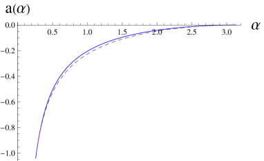
Figure 6: Plot of $a(\alpha)$ vs. $\alpha$. Continuous curve corresponds to the extrapolation of $a(\alpha)$ eq.(22) obtained by exact diagonalization of the $F_{\mathcal{D}}$ matrix. Dashed curve corresponds to the theoretical approximation for $a(\alpha)$ in eq.(32).

Fig.(6) shows the overlap between the extrapolation $a(\alpha)$ in (22) obtained by diagonalization of the $F_{\mathcal{D}}$ matrix and the theoretical expression (32). The small difference between the curves is due to the approximation done in the calculation of $TrF_{\mathcal{D}}^{2}$ (see eq.(45) in the Appendix).

In conclusion, in this section we have proof the validity of our proposal equation (LABEL:generalgam) for the entanglement entropy in a non-smooth domain.

IV Entanglement spectrum

The reduced density matrix $\mathcal{D}$ of a domain contains of course much more information that the entropy $S_{\mathcal{D}}$. In the context of the QHE this information is related to the physical degrees of freedom of the edge excitations, as proposed in reference hald . This is a rather surprising conjecture since, after all, the edge of $\mathcal{D}$ is an arbitrary curve within the whole system. The entanglement Hamiltonian, $H_{\mathcal{D}}$, defined as $\rho_{\mathcal{D}}=e^{-H_{\mathcal{D}}}$, is then expected to be intimately related to the Hamiltonian describing the excitations of a real edge. In the QHE the edge excitations are described by a chiral CFT, which also describes the excitations of the bulk. For the IQHE this result follows from the entanglement spectrum that is given by the eigenvalues of the operator gd

$$Q_{\mathcal{D}}=(1/2)-C_{\mathcal{D}},$$ (33)

with $C_{\mathcal{D}}$ the two point correlator defined in (7). In the smooth domain $\mathcal{D}_{0}$ (obtained considering $l_{x}=0$ in fig.1), the eigenvalues of $C_{\mathcal{D}_{0}}$ are given by eq.(10), so the entanglement spectrum will be:

$$q_{n}=\frac{1}{2}Erf\left(\frac{2\pi n}{L_{y}}\right)\ ,$$

$$n=-\infty,...,\infty\ ,$$ (34)

with $q_{n}$ the eigenvalues of $Q_{\mathcal{D}_{0}}$. In the limit $L_{y}>>1$, this spectrum becomes $q_{n}=2\sqrt{\pi}n/L_{y}$, which is that of a free chiral boson moving on a circle of length $L_{y}$ with a velocity $v=1/\sqrt{\pi}$. If we now deform the domain as in fig. 2, the entanglement spectrum in the boundary of $\mathcal{D}$ can be obtained from eq. (25)

$$q^{\prime}_{n}=\frac{1}{2}Erf\left(\frac{2\pi n(1-\kappa(l_{x},L_{y})}{L_{y}}\right)\ ,$$

$$n=-\infty,...,\infty\ .$$ (35)

In the limit $L_{y}>>1$, eq.(27) implies $P_{\mathcal{D}}=L_{y}/(1-\kappa(l_{x},L_{y}))$, and the spectrum (35) becomes $q^{\prime}_{n}=2\sqrt{\pi}n/P_{\mathcal{D}}$ which is that of a free chiral boson moving on a circle of length $P_{\mathcal{D}}$ with a velocity $v=1/\sqrt{\pi}$. That circle has the same length as the boundary of $P_{\mathcal{D}}$. The latter boundary has two singular points on it, i.e. two vertices with angles $\alpha$ and $2\pi-\alpha$, but they have subleading effects both on the entropy $S_{\mathcal{D}}$ and the entanglement spectrum. This phenomena is analogue to what happens for real systems where the electrons surround the hills and valleys of the potential travelling all the way through the sample.

In summary, we have computed in this paper the subleading term to the area law for IQHE states on polygonal domains, which is given by the expression

$$\gamma=\sum_{i}a(\alpha_{i})*n_{i}$$ (36)

where $n_{i}$ is the number of vertices in the domain with angle $\alpha_{i}$ and $a(\alpha_{i})$ is a function that only depends on the angles of the vertices and the density of the fluid. For the IQHE with filling fraction $\nu=1$, we have found numerical and analytical expressions of the function $a(\alpha)$, given by eqs. (22) and (32), which agree rather well. The fact that the correction (36) is a constant has its origin in the gapped character of the IQHE. For gapless 2+1 systems one may expect a size dependent subleading term. Indeed, this has been confirmed for relativistics free bosons and fermions in ref.CH and in an interacting CFT using the AdS/CFT conjecture in Ads . Also, the critical models with dynamical exponent $z=2$ of Fradkin and Moore FradMoore , exhibit a logarithmic subleading correction of the form

$$\beta=f(\alpha)*Log(L)$$ (37)

with $L$ the perimeter of the domain and $\alpha$ the angle of the vertex. The function $f(\alpha)$ has a similar behavior as $a(\alpha)$, in the sense that both curves satisfy $f(\alpha),a(\alpha)\leq 0$ and $\frac{\partial f(\alpha)}{\partial\alpha},\frac{\partial a(\alpha)}{\partial\alpha}\geq 0$. These properties are a consequence of the strong subadditivity relation satisfied by the entanglement entropy Ads .

Finally, we have obtained the entanglement spectrum of non smooth domains which corresponds to a chiral free boson moving on the boundary, in agreement with the conjecture of reference hald .

Acknowledgments We thank J.K. Slingerland and M. Haque for helpful comments. This work has been supported by Science Foundation Ireland through PI Award 08/IN.1/I1961 (I. D. R.) and the spanish project FIS2009-11654 (G.S.). We also acknowledge ESF Science Programme INSTANS 2005-2010.

Appendix

In this Appendix we calculate the trace (29) analytically. Let us first write it as

$$TrF^{2}_{\mathcal{D}_{A}\cup\mathcal{D}_{B}}=TrF^{2}_{\mathcal{D}_{A}}+TrF^{2}_{\mathcal{D}_{B}}+2Tr\left(F_{\mathcal{D}_{A}}F_{\mathcal{D}_{B}}\right)\ ,$$

(38)

with $\mathcal{D}_{A}$ and $\mathcal{D}_{B}$ given in fig.1. From the definition of $F_{\mathcal{D}}$ (see eq.(17)), the first term in (38) reads

$$TrF^{2}_{\mathcal{D}_{A}}=\int\int_{\mathcal{D}_{A}}d^{2}r^{\prime}\,d^{2}r\sum^{n_{0}}_{m,n=-n_{0}}\bar{\phi}_{m}(x^{\prime},y^{\prime})\phi_{n}(x^{\prime},y^{\prime})\times$$

$$\bar{\phi}_{n}(x,y)\phi_{m}(x,y)=\frac{1}{4\pi^{2}}\int\int_{\mathcal{D}_{A}}e^{-\frac{1}{2}(x-x^{\prime})^{2}-\frac{1}{2}(y-y^{\prime})^{2}}=$$

$$\int^{\frac{l_{x}}{2}}_{-\frac{l_{x}}{2}}dxdx^{\prime}\left(\frac{e^{-\frac{1}{2}(x-x^{\prime})^{2}-\frac{1}{8}a^{2}(l_{x}+x+x^{\prime})^{2}}}{2\pi^{2}}-\frac{e^{-\frac{1}{8}(4+a^{2})(x-x^{\prime})^{2}}}{2\pi^{2}}\right.$$

$$+\left.\frac{ae^{-\frac{1}{2}(x-x^{\prime})^{2}}(x^{\prime}-x)Erf\left[\frac{a(x-x^{\prime})}{2\sqrt{2}}\right]}{4\sqrt{2}\pi^{3/2}}+\frac{ae^{-\frac{1}{2}(x-x^{\prime})^{2}}}{4\sqrt{2}\pi^{3/2}}\times\right.$$

$$\left.(l_{x}+x+x^{\prime})Erf\left[\frac{a(l_{x}+x+x^{\prime})}{2\sqrt{2}}\right]\right)=A+B+C+D\ ,$$

(39)

where $a=\frac{L_{y}}{l_{x}}$. The integrals $A$ and $B$ in (39) can be easily found

$$A = \frac{\pi+2\arctan\left[\frac{1}{a}-\frac{a}{4}\right]}{4\pi^{2}a}\ ,$$

$$B = \frac{4}{(4+a^{2})\pi^{2}}-\frac{\sqrt{2}\,l_{x}}{\sqrt{4+a^{2}}\pi^{3/2}}\ .$$ (40)

To compute the integral $C$ we first integrate the variables $y,y^{\prime}$ and $x$ obtaining that:

$$C=\int_{-\frac{l_{x}}{2}}^{\frac{l_{x}}{2}}dx^{\prime}\left(\frac{a}{2\sqrt{2}\pi^{3/2}}e^{-\frac{1}{8}(l_{x}-2x^{\prime})^{2}}Erf\left[\frac{a(l_{x}-2x^{\prime})}{4\sqrt{2}}\right]\right.$$

$$-\left.\frac{a^{2}}{2\pi^{3/2}\sqrt{2(4+a^{2})}}Erf\left[\frac{\sqrt{4+a^{2}}(l_{x}-2x^{\prime})}{4\sqrt{2}}\right]\right)=$$

$$C_{1}+C_{2}\ .$$ (41)

The integral $C_{1}$ only depends on the ratio $a=L_{y}/l_{x}$. Therefore if we vary $l_{x}$, maintaining the value of $a$ constant (by adjusting $L_{y}$), the integral $C_{1}$ remains the same. Taking the limit $l_{x}\rightarrow\infty$ in $C_{1}$ and making the change of variables $u=l_{x}-2x^{\prime}$, one obtains an integral between $0$ and $\infty$ whose value is

$$C_{1}=\frac{a}{2\pi^{2}}\arctan\left[\frac{a}{2}\right]\ .$$ (42)

The integral $C_{2}$ is easily done

$$C_{2}=\frac{a^{2}}{(4+a^{2})\pi^{2}}-\frac{a^{2}l_{x}}{2\sqrt{2(4+a^{2})}\pi^{3/2}}\ .$$ (43)

Collecting the previous expressions one gets

$$C=\frac{a}{2\pi^{2}}\arctan\left[\frac{a}{2}\right]+\frac{a^{2}}{(4+a^{2})\pi^{2}}-\frac{a^{2}l_{x}}{2\sqrt{2(4+a^{2})}\pi^{3/2}}\ .$$

(44)

The integral $D$ in (39):

$$D=\int^{\frac{l_{x}}{2}}_{-\frac{l_{x}}{2}}\frac{ae^{-\frac{1}{2}(x-x^{\prime})^{2}}(l_{x}+x+x^{\prime})Erf\left[\frac{a(l_{x}+x+x^{\prime})}{2\sqrt{2}}\right]}{4\sqrt{2}\pi^{3/2}}\ .$$

(45)

cannot be solved analytically. However, one can obtain a very good approximation replacing in (45) $(l_{x}+x+x^{\prime})Erf\left[\frac{a(l_{x}+x+x^{\prime})}{2\sqrt{2}}\right]$ by $(l_{x}+x+x^{\prime})$, which upon integration yields

$$D=-\frac{al_{x}}{2\sqrt{2}\pi^{3/2}}+\frac{al_{x}^{2}}{4\pi}\ .$$ (46)

Finally, from (40),(44) and (46) we arrive at:

$$TrF^{2}_{\mathcal{D}_{A}}=\frac{\pi+2\arctan\left[\frac{1}{a}-\frac{a}{4}\right]}{4\pi^{2}a}\ +\frac{4}{(4+a^{2})\pi^{2}}-$$

$$\frac{\sqrt{2}l_{x}}{\sqrt{4+a^{2}}\pi^{3/2}}+\frac{a}{2\pi^{2}}\arctan\left[\frac{a}{2}\right]+\frac{a^{2}}{(4+a^{2})\pi^{2}}-$$

$$\frac{a^{2}l_{x}}{2\sqrt{2(4+a^{2})}\pi^{3/2}}-\frac{al_{x}}{2\sqrt{2}\pi^{3/2}}+\frac{al_{x}^{2}}{4\pi}\ .$$ (47)

To complete the calculation one needs the quantities $TrF^{2}_{\mathcal{D}_{B}}$ and $2Tr\left(F_{\mathcal{D}_{A}}F_{\mathcal{D}_{B}}\right)$ in (38). Their values are easy to obtain and they read

$$TrF^{2}_{\mathcal{D}_{B}}=\sum_{n}\left(F_{\mathcal{D}_{B}}\right)_{nn}\left(F_{\mathcal{D}_{B}}\right)_{nn}=n_{0}-\frac{L}{2\sqrt{2}\pi^{3/2}}-\frac{Ll_{x}}{4\pi}$$

$$TrF_{(\mathcal{D}_{A}\mathcal{D}_{B})}=\sum_{n}\left(F_{\mathcal{D}_{A}}\right)_{nn}\left(F_{\mathcal{D}_{B}}\right)_{nn}=\frac{L}{2\sqrt{2}\pi^{3/2}}-\frac{L}{8l_{x}\pi},$$

(48)

with $n_{0}$ defined in (2). In (48) we have used the fact that in the domain $\mathcal{D}_{B}$, the matrix $F$ is diagonal.

Finally, from (47) and (48) we obtain that:

$$TrF^{2}_{\mathcal{D}_{A}\cup\mathcal{D}_{B}}=-\frac{P_{\mathcal{D}_{A}\cup\mathcal{D}_{B}}}{2\sqrt{2}\pi^{3/2}}+n_{0}+\frac{4}{(4+a^{2})\pi^{2}}+\frac{a^{2}}{(4+a^{2})\pi^{2}}$$

$$+\frac{1}{4a\pi}-\frac{a}{4\pi}+\frac{\arctan\left[\frac{1}{a}-\frac{a}{4}\right]}{2a\pi^{2}}+\frac{a\arctan\left[\frac{a}{2}\right]}{2\pi^{2}}\ ,$$ (49)

with $P_{\mathcal{D}_{A}\cup\mathcal{D}_{B}}$ the perimeter of the domain $\mathcal{D}$ in fig.1. Observe from fig.1 that the ratio $a=\frac{L_{y}}{lx}$ is related with the angle, $\alpha$, of the vertex by $a=2Tan(\alpha/2)$. Therefore we can write eq.(49) in terms of the angle $\alpha$ obtaining that:

$$TrF^{2}_{\mathcal{D}_{A}\cup\mathcal{D}_{B}}=-\frac{P_{\mathcal{D}_{A}\cup\mathcal{D}_{B}}}{2\sqrt{2}\pi^{3/2}}+n_{0}$$

$$+\frac{4+(\pi-\alpha)(-1+3\cos(\alpha))\csc(\alpha)}{4\pi^{2}}\ .$$ (50)

References

- (1) L. Amico, R. Fazio, A. Osterloh and V. Vedral, ”Entanglement in Many-Body Systems”, Rev. Mod. Phys. vol. 80, 517-576 (2008); arXiv:quant-ph/0703044.
- (2) M.M. Wolf, F. Verstraete, M.B. Hastings and J.I. Cirac, ”Area laws in quantum systems: mutual information and correlations”, Phys. Rev. Lett. 100, 070502 (2008); arXiv:0704.3906.
- (3) J. Eisert, M. Cramer and M.B. Plenio, ”Area laws for the entanglement entropy - a review”, Rev. Mod. Phys. 82, 277 (2010); arXiv:0808.3773.
- (4) C. Holzhey, F. Larsen and F. Wilczek, ”Geometric and Renormalized Entropy in Conformal Field Theory”, Nucl. Phys. B424, 443 (1994); arXiv:hep-th/9403108.
- (5) G. Vidal, J. I. Latorre, E. Rico and A. Kitaev, ”Entanglement in quantum critical phenomena”, Phys. Rev. Lett. 90, 227902 (2003); arXiv:quant-ph/0211074.
- (6) B.-Q.Jin and V.E.Korepin, ”Quantum Spin Chain, Toeplitz Determinants and Fisher-Hartwig Conjecture”, J. Stat. Phys. 116, Nos. 1-4, 79 (2004); arXiv:quant-ph/0304108.
- (7) P. Calabrese and J. Cardy, ”Entanglement Entropy and Quantum Field Theory”, J. Stat. Mech. (2004) P06002; arXiv:hep-th/0405152.
- (8) P. Calabrese, M. Campostrini, F. Essler and B. Nienhuis, ”Parity effects in the scaling of block entanglement in gapless spin chains”, Phys.Rev.Lett.104, 095701 (2010); arXiv:0911.4660.
- (9) J. Cardy and P. Calabrese, ”Unusual Corrections to Scaling in Entanglement Entropy”, J. Stat. Mech. (2010) P04023; arXiv:1002.4353.
- (10) A. Kitaev and J. Preskill, ”Topological entanglement entropy”, Phys. Rev. Lett. 96, 110404 (2006); arXiv:hep-th/0510092.
- (11) M. Levin and X. G. Wen, ”Detecting topological order in a ground state wave function”, Phys. Rev. Lett. 96, 110405 (2006); arXiv:cond-mat/0510613.
- (12) M. Haque, O. Zozulya and K. Schoutens, ”Entanglement entropy in fermionic Laughlin states”, Phys. Rev. Lett. 98, 060401 (2007); arXiv:cond-mat/0609263.
- (13) O.S. Zozulya, M. Haque, K. Schoutens and E.H. Rezayi, ”Bipartite entanglement entropy in fractional quantum Hall states” Phys. Rev. B76, 125310 (2007); arXiv:0705.4176.
- (14) A. Laeuchli, E. J. Bergholtz and M. Haque, ”Entanglement Scaling of Fractional Quantum Hall states through Geometric Deformations”; arXiv:1003.5656.
- (15) B. A. Friedman and G. C. Levine, ”Topological entropy of realistic quantum Hall wave functions”, Phys. Rev. B 78,035320 (2008); arXiv:0710.4071.
- (16) S. Dong, E. Fradkin, R. G. Leigh and S. Nowling, ”Topological Entanglement Entropy in Chern-Simons Theories and Quantum Hall Fluids”, JHEP 0805: 016 (2008); arXiv:0802.3231.
- (17) T. Barthel, M.C. Chung and U. Schollwock, ”Entanglement scaling in critical two-dimensional fermionic and bosonic systems”, Phys. Rev. A 74, 022329 (2006);arXiv:cond-mat/0602077.
- (18) M. Cramer, J. Eisert and M.B. Plenio, ”Statistics dependence of the entanglement entropy”, Phys.Rev.Lett.98:220603 (2007); arXiv:quant-ph/0611264v4.
- (19) S. Farkas and Z. Zimboras, ”The von Neumann entropy asymptotics in multidimensional fermionic systems”, J. Math. Phys. 48, 102110 (2007); arXiv:0706.1805v1.
- (20) D. Gioev and I. Klich, ”Entanglement entropy of fermions in any dimension and the Widom conjecture”, Phys. Rev. Lett. 96, 100503 (2006); arXiv:quant-ph/0504151.
- (21) W. Li, L. Ding, R. Yu, T. Roscilde and S. Haas, ”Scaling Behavior of Entanglement in Two- and Three-Dimensional Free Fermions”, Phys.Rev. B 73, 064406 (2006); arXiv:quant-ph/0602094.
- (22) M. M. Wolf, ”Violation of the entropic area law for Fermions”, Phys. Rev. Lett. 96, 010404 (2006); arXiv:quant-ph/0503219.
- (23) F. D. M. Haldane, ”Luttinger’s Theorem and Bosonization of the Fermi Surface”, in Perspectives in Many-Particle Physics, eds. R. Broglia and J. R. Schrieffer, (North Holland, Amsterdam 1994, pp 5-30); cond-mat/0505529.
- (24) H.Casini and M.Huerta, ”Entanglement entropy in free quantum field theory”, J.Phys.A42:504007 (2009); airxiv:0905.2562v3 and H. Casini, M. Huerta and L. Leitao, ”Entanglement entropy for a Dirac fermion in three dimensions: vertex contribution”, Nucl.Phys.B814:594-609 (2009); arxiv:hep-th/0811.1968.
- (25) T. Hirata and T. Takayanagi, ”AdS/CFT and Strong Subadditivity of Entanglement Entropy”, JHEP 0702, 042 (2007); arXiv:hep-th/0608213.
- (26) E. Fradkin and J. E. Moore, ”Entanglement entropy of 2D conformal quantum critical points: hearing the shape of a quantum drum”, Phys.Rev.Lett.97, 050404 (2006); airxiv:cond-mat/0605683.
- (27) B. Hsu, M. Mulligan, E. Fradkin, and E. A. Kim, ”Universal entanglement entropy in 2D conformal quantum critical points”, Phys. Rev. B, 79, 115421 (2009); arXiv:0812.0203; E. Fradkin, ” Scaling of Entanglement Entropy at 2D quantum Lifshitz fixed points and topological fluids”, Journal of Physics A: Math. Theor. 42, 504011 (2009); arXiv:0906.1569; and B. Hsu and E. Fradkin, ”Universal Behavior of Entanglement in 2D Quantum Critical Dimer Models”; arXiv:1006.1361.
- (28) I. Peschel, ”Calculation of reduced density matrices from correlation functions”, J.Phys. A: Math. Gen. 36, L205 (2003); arXiv:cond-mat/0212631.
- (29) Ivan D. Rodriguez and German Sierra, ”Entanglement entropy of integer Quantum Hall states”, Phys.Rev. B vol. 80, 153303 (2009); arXiv:0811.2188.
- (30) H. Li and F. D. M. Haldane, ”Entanglement Spectrum as a Generalization of Entanglement Entropy: Identification of Topological Order in Non-Abelian Fractional Quantum Hall Effect States”, Phys. Rev. Lett. 101, 010504 (2008); arXiv:0805.0332.
- (31) M.A. Turner, Y. Zhang and A. Vishwanath, ”Band Topology of Insulators via the Entanglement Spectrum”; arXiv:0909.3119.
- (32) R. Thomale, A. Sterdyniak, N. Regnault and B. A. Bernevig, ”The entanglement gap and a new principle of adiabatic continuity”, Phys. Rev. Lett. 104, 180502 (2010); arXiv:0912.0523 and A. Sterdyniak, N. Regnault and B.A. Bernevig, ”Extracting Excitations From Groundstate Entanglement”; arXiv:1006.5435.