Viscoresistive MHD Configurations of Plasma in Accretion Disks

Abstract.

We present a discussion of two-dimensional magneto-hydrodynamics (MHD) configurations, concerning the equilibria of accretion disks of a strongly magnetized astrophysical object. We set up a viscoresistive scenario which generalizes previous two-dimensional analyses by reconciling the ideal MHD coupling of the vertical and the radial equilibria within the disk with the standard mechanism of the angular momentum transport, relying on dissipative properties of the plasma configuration.

The linear features of the considered model are analytically developed and the non-linear configuration problem is addressed, by fixing the entire disk profile at the same order of approximation. Indeed, the azimuthal and electron force balance equations are no longer automatically satisfied when poloidal currents and matter fluxes are included in the problem. These additional components of the equilibrium configuration induce a different morphology of the magnetic flux surface, with respect to the ideal and simply rotating disk.
PACS:97.10.Gz; 95.30.Qd; 52.30.Cv

1. Preliminaries

Understanding the mechanism of accretion that compact objects show in the presence of lower dense companions, is a long standing problem in astrophysics (Bisnovatyi-Kogan and Lovelace, 2001). In fact, while in absence of a significant magnetic field of the massive body the disk configuration is properly described by the fluidodynamical approach (Shakura, 1973), the situation becomes a bit puzzling when we deal with a strongly magnetized source. Since over the last three decades, increasing interest raised about the mechanism of the angular momentum transport across the disk profile. The solution of this problem stands as settled down in the form of a standard model, at least in the case of small (intrinsic) magnetic fields. This context prevents the formation of high magnetic back-reactions inside the plasma disk and the gas-like approximation is predictive. We remark how it is known from the observations (Verbunt, 1982) that the accretion profile takes place often with the morphology of a thin disk configuration. In this limit of a thin gaseous disk, the hydrodynamical equilibria underlying the accretion process are cast into a one-dimensional paradigm, (see among the first analyses of the problem (Pringle and Rees, 1972; Shakura, 1973; Lynden-Bell and Pringle, 1974)). In such a fluidodynamical scenario, the accretion mechanism relies on the angular momentum transfer as allowed by the shear viscosity properties of the disk material. The differential angular rotation of the radial layers is associated with a non-zero viscosity coefficient, accounting for diffusion and turbulence phenomena. Indeed, microscopic estimations of the viscosity parameter indicate that the friction of different disk layers would be unable to maintain a sufficiently high accretion rate, and therefore non-linear turbulent features of the equilibrium are inferred.

However, when the magnetic field $\vec{B}$ of the central object is strong enough, the electromagnetic back-reaction of the disk plasma becomes relevant (Ruffini and Wilson, 1975). As shown in Coppi (2005), the Lorentz force induces a coupling between the radial and the vertical equilibria, which deeply alters the local morphology of the system. In particular, the radial dependence of the disk profile acquires an oscillating character, modulating the background structure too. The existence of such a coupling breaks down the one-dimensional nature of the problem and suggests a revision of the original point of view of the standard model.

Furthermore, in Coppi and Rousseau (2006) it is discussed how the plasmas, characterised by a $\beta$-parameter (i.e. the ratio of the thermostatic pressure $p$ to the magnetic one $B^{2}/8\pi$) close to unity, exhibit an oscillating-like mass density and the disk is decomposed in a ring profile. Thus, the analyses in Coppi (2005); Coppi and Rousseau (2006) demonstrate that the details of the disk equilibria are relevant in establishing a crystalline local structure inside the disk. This ideal MHD result constitutes an opposite point of view with respect to the idea of a diffusive magnetic field within the disk, as discussed in Bisnovatyi-Kogan and Lovelace (2001). The striking interest in the details of this local disk morphology relies on the idea that jets of matter and radiation are emitted by virtue of the strong magnetic field and of the axial symmetry of the accretion profiles (see for instance Lynden-Bell (1996)).

Such an ideal two-dimensional MHD analysis is pursued by neglecting the accretion rate of the disk in the leading order (see also the global analysis presented in Ogilvie (1997)) and thus without facing the question about the azimuthal balance of the forces acting on the electrons. In fact, in these works (Ogilvie, 1997; Coppi, 2005; Coppi and Rousseau, 2006), toroidal currents (and toroidal matter fluxes) are addressed only. We analyze in some detail the implications that accounting for the azimuthal and electron force balance equilibrium equations has on the local profile of the disk. We pursue the setting up of these two additional equations in the same approximation limit of the analysis in Coppi (2005) and in Coppi and Rousseau (2006) and we arrive to establish a direct relation between the radial infall velocity and the azimuthal Lorentz force. This result relies on addressing a link between the turbulent viscosity coefficient and the resistivity one. In particular, in the limiting case $\beta\to\infty$, we are able to fix the vertical dependence of the plasma configuration, differently from the issue in Coppi (2005), for the same limiting case. The radial velocity we derive this way has an oscillating behavior in its radial dependence and therefore has a zero net radial average. This matter infall profile is able to provide a local non-zero accretion rate and therefore it reconciles the crystal structure, outlined in Coppi (2005), with a real accretion feature active in the disk.

The paper is organized as follows. In subsection 1.1 we describe the basic equations of the stationary MHD. In subsection 1.2 the standard hydrodynamic theory of accretion disk is presented. In Section 2 the bidimensional accretion disk is discussed in the framework of MHD. Section 3 is devoted to an analysis of the azimuthal equation and on the balance of the force acting on the electrons along the tangential direction. The linear approximation of this bidimensional model is discussed in Section 4, while the non linear configuration is developed in Section 5. Concluding Remarks follow

1.1. MHD of the Steady State

The behavior of a plasma embedded into a magnetic and a gravitational fields can be described by a MHD approach for a wide range of configurations. In the case of hydrogen-like ions and when a steady state holds, the system configuration is governed by the following set of equations (as written in Cartesian coordinates, and we note that repeated indices are intended as summed).

(1a) $$\partial_{i}\left(\epsilon v_{i}\right)=0$$

(1b) $$\epsilon v_{l}\partial_{l}v_{i}=-\partial_{i}p+\partial_{l}\left[\mathcal{D}\left(\partial_{i}v_{l}+\partial_{l}v_{i}-\displaystyle\frac{2}{3}\delta_{il}\partial_{k}v_{k}\right)\right]-\partial_{i}\chi+\displaystyle\frac{1}{c}\epsilon_{ijk}J_{j}B_{k}$$

(1c) $$v_{l}\partial_{l}T+\displaystyle\frac{2}{3}T\partial_{l}v_{l}=0\,,$$

where the mass density $\epsilon$ and the total (electron plus ion) pressure $p$ are related via the temperature $T$, according to the equation of state $p=2KT\epsilon/m$, where $K$ denotes the Boltzmann constant and $m$ is the proton mass. Here $\mathcal{D}$ denotes the shear viscosity coefficient, $J_{i}$ the density current vector, $v_{i}$ the plasma velocity field, while, $\chi$ stands for the Newton potential due to the central body of mass $M_{\mathrm{S}}$ (the self-gravity of the plasma being negligible), i.e. $\chi(x^{i})=GM_{\mathrm{S}}/\sqrt{\delta_{ij}x^{i}x^{j}}$. Instead, the plasma acquires an internal electromagnetic structure whose back-reaction can be relevant.

The behavior of the total electric field $E_{i}$ and magnetic field $B_{i}$ is described by the Maxwell equations standing in Gaussian units as

(2a) $$\epsilon_{ijk}\partial_{j}B_{k}=\displaystyle\frac{4\pi}{c}J_{i}$$

(2b) $$\partial_{l}E_{l}=4\pi\rho$$

(2c) $$\epsilon_{ijk}\partial_{j}E_{k}=0\quad\Rightarrow\quad E_{i}=-\partial_{i}\Phi$$

(2d) $$\partial_{l}B_{l}=0\quad\Rightarrow\quad B_{i}=\epsilon_{ijk}\partial_{j}A_{k} \,,$$

where $A_{i}$ denotes the potential vector, $\rho$ the electric charge density, $\Phi$ the electric potential and the electric and magnetic fields are related by the MHD condition

(3) $$E_{l}=-\displaystyle\frac{1}{c}\epsilon_{lmn}v_{m}B_{n}\,.$$

Recalling the relation

(4) $$\epsilon_{ijk}\epsilon_{ilm}=\delta_{jl}\delta_{km}-\delta_{jm}\delta_{kl}$$

and by means of Eq.(2a) the Lorentz force rewrites as

(5) $$\frac{1}{c}\epsilon_{ijk}J_{j}B_{k}=\displaystyle\frac{1}{4\pi}\left(-B_{l}\partial_{i}B_{l}+B_{l}\partial_{l}B_{i}\right)\,.$$

The scheme we traced above completely fixes the steady plasma configuration, once assigned the central object morphology.

1.2. The Standard Model of Accretion disks

The characterization of an accretion disk is obtained by addressing an axisymmetric MHD configuration (described by cylindrical coordinates $r,\,\phi,\,z$) for the plasma surrounding the central object. However, some fundamental features of the accretion process are fixed by the fluidodynamical approach describing the matter infall through a gas disk profile, as outlined in Shakura (1973). We aim to fix how the viscoresistive approach is not well-grounded on a microscopical level and a new perspective is required, as based on typical features observed in laboratory plasmas (Coppi, 2005; Coppi and Rousseau, 2006).

In the standard model of accretion, the configuration of an axisymmetric thin disk is determined by the fluidodynamical equilibria, which take place within the central gravitational field.

The thin character of the disk depth allows us to simplify the configuration problem, by integrating over the vertical profile, so fixing an effective one-dimensional hydrodynamical problem. When averaged out of the vertical direction (Bisnovatyi-Kogan and Lovelace, 2001), the radial equilibrium reduces to the condition that the angular velocity $\omega$ of the disk takes the Keplerian profile

(6) $$\omega(r)=\omega_{\mathrm{K}}=\sqrt{\frac{GM_{\mathrm{S}}}{r^{3}}}\,.$$

This statement is equivalent to neglect the role played in the equilibrium by the radial pressure gradient, retaining the centripetal force exerted by the central object as the dominant effect. This Keplerian nature of the disk is well-grounded and significant deviations from such a behavior are expected in advective dominated regimes only.

The vertical equilibrium corresponds to the gravothermal configuration confining the disk profile, and it is therefore governed by the equation

(7) $$\frac{dp}{dz}+\omega^{2}_{\mathrm{K}}z\epsilon=0\,,$$

which, for an isothermal disk of temperature $T$ and equation of state $p=v_{\mathrm{s}}^{2}\epsilon$ (where $v_{\mathrm{s}}^{2}=2K_{\mathrm{B}}T/m$ is the sound velocity), gives the exponential decay of the mass density over the equatorial plane value $\epsilon_{0}(r)$, i.e.

(8) $$D(z^{2})\equiv\frac{\epsilon}{\epsilon_{0}}=\exp\left(-\displaystyle\frac{z^{2}}{H^{2}}\right)\,.$$

Here, $H=\sqrt{2v_{\mathrm{s}}^{2}/\omega_{\mathrm{K}}^{2}}$ provides an estimation for the real half-depth of the disk, which, in principle would have an infinite vertical extension.

The azimuthal equilibrium describes the angular momentum transport across the disk, by virtue of a viscous stress tensor component $\tau_{r\phi}$ which enters the relation (first integral of the azimuthal equation)

(9) $$\dot{M}_{\mathrm{d}}(L-L_{\mathrm{d}})=-2\pi r^{2}\tau_{r\phi}\quad,\quad\tau_{r\phi}=\mathcal{D}r^{2}\frac{d\omega}{dr}\,.$$

Here $\mathcal{D}$ must be thought as a turbulent viscosity coefficient, while $L$ is the angular momentum per unit mass. Moreover, $L_{\mathrm{d}}$ is a fixed value of the specific angular momentum and

(10) $$\dot{M}_{\mathrm{d}}\equiv-2\pi r\int_{-H}^{H}(\epsilon v_{r})dz=-2\pi r\sigma v_{r}\,,$$

is the mass accretion rate, associated to the radial velocity $v_{r}<0$ and to the surface mass density $\sigma\equiv\int_{-H}^{H}\epsilon dz$. Finally the continuity equation

(11) $$\frac{1}{r}\frac{d(r\epsilon v_{r})}{dr}+\frac{d(\epsilon v_{z})}{dz}=0\,,$$

once integrated over the vertical direction provides with the fundamental relation $\dot{M}_{\mathrm{d}}=\mathrm{const}>0$.

Recalling that the model is dominated by the Keplerian feature $\omega\simeq\omega_{\mathrm{K}}$ and observing that $d\omega_{\mathrm{K}}/dr=-3\omega_{\mathrm{K}}/2r$, we arrive to the following form for the angular momentum transport versus the plasma turbulent viscosity

(12) $$\dot{M}_{\mathrm{d}}(L-L_{\mathrm{d}})=3\pi\mathcal{D}\omega_{\mathrm{K}}r^{2}\,.$$

Plasma viscosity

This picture of the accretion mechanism is however affected by a discrepancy between theory and observations of real systems. In fact, the viscosity coefficient $\mathcal{D}$ in the disk is too small if estimated by the microscopic plasma (or atomic) structure. Its microscopic features are unable to account for the accretion rates observed in some astrophysical systems, like X-ray binaries. The observed accretion rates, as estimated by the increasing disk luminosity ${\dot{\mathcal{L}}}_{\mathrm{d}}\sim GM_{\mathrm{S}}{\dot{M}}_{\mathrm{d}}/r_{\mathrm{S}}$ ($r_{\mathrm{S}}$ being the radius of the central object), would require a larger value of $\mathcal{D}$, (see the discussion in Shakura (1973)). The solution to this discrepancy is inferred in the turbulent behavior arising in the disk when the Reynold number is sufficiently large. Such turbulence in the disk plasma would then be responsible for the appearance of the large value of the viscosity coefficient.

Since, by definition $L=\omega r^{2}$, we can infer

(13) $$\mathcal{D}=2\sigma v_{\mathrm{t}}H/3\,,$$

$v_{\mathrm{t}}$ being a turbulence velocity, given by $v_{\mathrm{t}}=\alpha v_{\mathrm{s}}$, where $\alpha$ is a free parameter. It must be noted that the axisymmetric disk is linearly stable with respect to small perturbations preserving its symmetry and the angular momentum conservation. For a discussion of the onset of turbulence by MHD instabilities, see the analysis presented in Balbus and Hawley (1998). Such a review work is based on the Velikhov approach of 1959 and it requires non-linear interaction among perturbations of very small amplitude.

1.3. Comparison with the literature

The difficulty of this turbulent scenario, led B. Coppi to provide in Coppi (2005) a local 2-dimensional MHD formulation of the disk profile, which argues how the notion of plasma turbulence could be replaced by microscopic ring-like structures. In this framework, that we address below, the effect of turbulent viscosity has to be replaced by fundamental plasma instabilities, observed in laboratory experiments, like the so-called Resistive Ballooning Modes. An interesting ideal two-dimensional MHD analysis of a rotating disk equilibrium has been provided by G. I. Ogilvie in Ogilvie (1997), where the thin disk configuration is addressed in both the weak and strong magnetic field limit (also solutions are derived assuming self-similarity in the radial profile of the non-thin case). The hypotheses at the ground of this work are the same as in Coppi (2005); Coppi and Rousseau (2006), but the analyzed regimes are significantly different. In fact, in Ogilvie (1997) the radial dependence of the disk profile has a power-law structure and the existence of the ring morphology does not emerge for a strongly magnetized thin disk. The main reason of such significant deviation between these two ideal MHD approaches relies both on the local character of the analysis of Coppi (compared to the global profile of Ogilvie) and on the nature of the asymptotic expansion of Ogilvie, which privileges the second vertical derivatives with respect to the radial ones (so altering the Laplacian term appearing in the local equilibria fixed by Coppi).

Our analysis differs from both these two ideal formulations of the axisymmetric MHD equilibria, not only for including dissipative effects (like viscosity and resistivity), but, overall in view of considering poloidal currents and matter fluxes. In fact in order to describe the accretion phenomenon it is necessary to deal with radially in-falling material and expectedly a non-zero azimuthal Lorentz force. These two features are not present in the approaches followed in Ogilvie (1997); Coppi (2005); Coppi and Rousseau (2006) and our generalization involves dissipative effects too in order to compare the vertical and radial coupling, within the disk configuration, to the paradigm of the standard approaches.

Indeed, the standard model treatment of the accretion process is properly reviewed by Bisnovatyi-Kogan and Lovelace (2001), where the main features of the disk morphology and the main successful issues are summarized in some detail. For a more recent analysis of the questions concerning the diffusive magnetic field living in the plasma configuration and its possible enhancement to get jet configuration see Spruit (2008). The models presented in these two reviews differ deeply from the analyses by Coppi or by Ogilvie, because the validity of the viscoresistive MHD approach is postulated on a phenomenological ground, almost disregarding the coupling between the radial and the vertical equilibria.

The main merit of our approach is in reconciling the two-dimensional MHD scenario, including microstructures of the plasma configuration, with the the viscoresistive formulation of the standard theory. Despite we are here not able to solve the resistivity puzzle (see the dedicated paragraph of section 3.1), we demonstrate that the microstructures determined by B. Coppi for the ideal MHD approach still survive in the presence of non-zero viscosity and resistivity coefficients and of the related radial and vertical matter velocity components. Demonstrating such a structural stability of the crystalline profile, we open the perspective to unify the microscopical and observational points of view, expectedly on the level of plasma instabilities. Anyway, the non-zero local accretion rate predicted by our model represents a significant improvement of the analysis in Coppi (2005); Coppi and Rousseau (2006), because it upgrades the crystalline picture toward a realistic disk configuration.

2. Two-Dimensional MHD Model for an Accretion Disk

Let us now specify the steady MHD theory, discussed in Section 2, to the specific case of an accretion disk configuration around the compact (few units of Solar mass) and strongly magnetized (a dipole-like field of about $10^{12}Gauss$), i.e. a typical pulsar source. The gravitational potential of the pulsar has the form

(14) $$\chi(r\,,z)=\frac{GM_{\mathrm{S}}}{\sqrt{r^{2}+z^{2}}}\,,$$

It is worth noting that the axial symmetry prevents any dependence on the azimuthal angle $\phi$ of all the quantities involved in the problem. In this respect the continuity equation takes the explicit form (11), which provides the following matter flux associated with the disk morphology

(15) $$\epsilon\vec{v}=-\frac{1}{r}\partial_{z}\Theta\vec{e}_{r}+\epsilon\omega(r\,,z^{2})r\vec{e}_{\phi}+\frac{1}{r}\partial_{r}\Theta\vec{e}_{z}\,,$$

where $\Theta(r\,,z)$ is an odd function of $z$ in order to deal with a non-zero accretion rate, i.e.

(16) $$\dot{M}_{\mathrm{d}}=-2\pi r\int_{-H}^{H}\epsilon v_{r}dz=4\pi\Theta(r\,,H)>0\,,$$

The magnetic field, characterizing the central object, takes the form

(17) $$\vec{B}=-\frac{1}{r}\partial_{z}\psi\vec{e}_{r}+\frac{I}{r}\vec{e}_{\phi}+\frac{1}{r}\partial_{r}\psi\vec{e}_{z}\,,$$

with $\psi=\psi(r\,,z^{2})$ and $I=I(\psi\,,z)$. The similarity of the magnetic field and matter flux structure, is due to their common divergence-less nature.

We now develop a local model of the equilibrium, as settled down around a radius value $r=r_{0}$, in order to analytically investigate the effects induced on the disk profile by the electromagnetic reaction of the plasma. To this end we split the mass density and the pressure contributions as $\epsilon=\bar{\epsilon}(r_{0},\,z^{2})+\hat{\epsilon}$ and $p=\bar{p}(r_{0},\,z^{2})+\hat{p}$, respectively. The same way, we express the magnetic surface function in the form $\psi=\psi_{0}(r_{0})+\psi_{1}(r_{0}\,,r-r_{0}\,,z^{2})$, with $\psi_{1}\ll\psi_{0}$. The quantities $\hat{\epsilon}$, $\hat{p}$ and $\psi_{1}$ describe the change induced by the currents which rise within the disk imbedded into the external magnetic field of the central object. In general these corrections are small in amplitude but with a very short scale of variation. Thus, we are lead to address the ”drift ordering” for the behavior of the gradient amplitude, i.e. the first order gradients of the perturbations are of zero-order, while the second order ones dominate.

As ensured by the corotation theorem Ferraro (1937), the angular frequency of the disk rotation has to be expressed via the flux function as $\omega(\psi)$. As a consequence, in the present split scheme, we can take the decomposition $\omega=\omega_{\mathrm{K}}+\omega^{\prime}_{0}\psi_{1}$, where $\omega_{\mathrm{K}}$ is the Keplerian term and $\omega^{\prime}_{0}=\mathrm{const}.$. This form for $\omega$ holds locally, as far as $(r-r_{0})$ remains a sufficiently small quantity, so that the dominant deviation from the Keplerian contribution is due to $\psi_{1}$.

Accordingly to the drift ordering, the profile of the toroidal currents rising in the disk, has the form

(18) $$J_{\phi}\simeq-\frac{c}{4\pi r_{0}}\left(\partial^{2}_{r}\psi_{1}+\partial_{z}^{2}\psi_{1}\right)\,.$$

On the other hand, the azimuthal component of the Lorentz force is related to the existence of the function $I(\psi,z)$ and it can be written as

(19) $$F_{\phi}\simeq\frac{1}{4\pi r_{0}^{2}}\left(\partial_{z}I\partial_{r}\psi-\partial_{r}I\partial_{z}\psi\right)\,.$$

2.1. Vertical and Radial Equilibria

We now fix the equations governing the vertical and the radial equilibrium of the disk, distinguishing the fluid components from the electromagnetic back-reaction (as develop by Coppi (2005); Coppi and Rousseau (2006)). Such a splitting of the MHD equations for the vertical force balance gives

(20) $$D(z^{2})\equiv\frac{\bar{\epsilon}}{\epsilon_{0}(r_{0})}=\exp\left(-\frac{z^{2}}{H^{2}}\right)\,,\hskip 14.22636pt\epsilon_{0}(r_{0})\equiv\epsilon(r_{0},\,0)\,,\hskip 14.22636ptH^{2}\equiv\frac{4K_{\mathrm{B}}\bar{T}}{m\omega_{\mathrm{K}}^{2}}\;,$$

(21) $$\partial_{z}\hat{p}+\omega^{2}_{\mathrm{K}}z\hat{\epsilon}-\frac{1}{4\pi r_{0}^{2}}\left(\partial^{2}_{z}\psi_{1}+\partial^{2}_{r}\psi_{1}\right)\partial_{z}\psi_{1}=0\,,$$

Here, as in Section 1.2, the behavior of the function $D(z^{2})$ accounts for the pure thermostatic equilibrium standing in the disk when the vertical gravity (i.e. the Keplerian rotation) is sufficiently high to provide a confined thin configuration, while the temperature $T$ admits the representation

(22) $$2K_{\mathrm{B}}T\equiv m\frac{p}{\epsilon}=m\frac{\bar{p}+\hat{p}}{\bar{\epsilon}+\hat{\epsilon}}\equiv 2K_{\mathrm{B}}(\bar{T}+\hat{T})\,.$$

The radial equation underlying the equilibrium of the rotating layers of the disk, can be decomposed into the dominant character of the Keplerian angular velocity plus an equation describing the behavior of the deviation $\delta\omega$, i. e.

(23) $$\omega\simeq\omega_{\mathrm{K}}+\delta\omega\simeq\omega_{0}(\psi_{0})+\omega_{0}^{\prime}\psi_{1}\;,$$

(24) $$\begin{split}2\omega_{\mathrm{K}}r_{0}(\bar{\epsilon}+\hat{\epsilon})\omega_{0}^{\prime}\psi_{1}&+\frac{1}{4\pi r_{0}^{2}}\left(\partial^{2}_{z}\psi_{1}+\partial^{2}_{r}\psi_{1}\right)\partial_{r}\psi_{1}=\\ &=\partial_{r}\left[\hat{p}+\frac{1}{8\pi r_{0}^{2}}\left(\partial_{r}\psi_{1}\right)^{2}\right]+\frac{1}{4\pi r_{0}^{2}}\partial_{r}\psi_{1}\partial^{2}_{z}\psi_{1}\end{split}$$

Here we neglected the presence of the poloidal currents, associated with the azimuthal component of the magnetic field.

Let us define the dimensionless functions $Y$, $\hat{D}$ and $\hat{P}$, in place of $\psi_{1}$, $\hat{\epsilon}$ and $\hat{p}$, i.e.

(25) $$Y\equiv\frac{k_{0}\psi_{1}}{\partial_{r_{0}}\psi_{0}}\,,\hskip 14.22636pt\hat{D}\equiv\frac{\beta\hat{\epsilon}}{\epsilon_{0}}\,,\hskip 14.22636pt\hat{P}\equiv\beta\frac{\hat{p}}{p_{0}}\,,$$

where $p_{0}\equiv 2K_{\mathrm{B}}\bar{T}\epsilon_{0}$ and $\beta\equiv 8\pi p_{0}/B^{2}_{0z}=1/(3\epsilon_{z}^{2})\equiv k_{0}^{2}H^{2}/3$. Here we introduced the fundamental wavenumber $k_{0}$ of the radial equilibrium, defined as $k_{0}\equiv 3\omega_{\mathrm{K}}^{2}/v_{\mathrm{A}}^{2}$, with $v_{\mathrm{A}}^{2}\equiv B^{2}_{z0}/4\pi\epsilon_{0}$, recalling that $B_{z0}=B_{z}(r,z=0)=\partial_{r_{0}}\psi_{0}/r_{0}$. Thus, we introduce the dimensionless radial variable $x\equiv k_{0}(r-r_{0})$, while we assume that the fundamental length in the vertical direction be $\Delta\equiv\sqrt{\epsilon_{z}}H$, leading to define $u\equiv z/\Delta$. By these definitions, the vertical equilibrium can be restated as

(26) $$\partial_{u^{2}}\hat{P}+\epsilon_{z}\hat{D}-2\left(\partial^{2}_{x}Y+\epsilon_{z}\partial^{2}_{u}Y\right)\partial_{u^{2}}Y=0\,,$$

while the radial configuration is fixed by

(27) $$\left(D+\frac{1}{\beta}\hat{D}\right)Y+\left(\partial^{2}_{x}Y+\epsilon_{z}\partial^{2}_{u}Y\right)(1+\partial_{x}Y)+\frac{1}{2}\partial_{x}\hat{P}=0\,.$$

The two equations above provide a coupled system for $\hat{P}$ and $Y$ once the quantities $D$ and $\hat{D}$ are assigned; hence we are able to determine the disk configuration induced by the toroidal currents. However, it remains to be described the accretion features of of the disk and the angular momentum transport across the crystalline structure lacking in the original analysis developed in Coppi (2005); Coppi and Rousseau (2006).

3. Azimuthal equation

The equilibrium along the toroidal symmetry of the disk is described by an equation which takes the exact expression

(28) $$\epsilon v_{r}\partial_{r}(\omega r)+\epsilon v_{z}\partial_{z}(\omega r)+\epsilon\omega v_{r}=\frac{1}{r^{2}}\partial_{r}\left(\mathcal{D}r^{3}\partial_{r}\omega\right)+\partial_{z}\left[\mathcal{D}\partial_{z}(\omega r)\right]+F_{\phi}\,,$$

$F_{\phi}$ being the $\phi$-component of the Lorentz force. The corotation theorem, stating $\omega=\omega(\psi)$, allows us to rewrite the equation above as

(29) $$\begin{split}&\epsilon rv_{r}\partial_{r}\psi+\epsilon rv_{z}\partial_{z}\psi+2\epsilon v_{r}\frac{\omega}{\omega^{\prime}}=\\ &\frac{1}{r^{2}\omega^{\prime}}\partial_{r}\left(\mathcal{D}r^{3}\omega^{\prime}\partial_{r}\psi\right)+\frac{1}{\omega^{\prime}}\partial_{z}\left[\mathcal{D}r\omega^{\prime}\partial_{z}\psi\right]+\frac{F_{\phi}}{\omega^{\prime}}\,,\end{split}$$

($\omega^{\prime}=d\omega/d\psi$). By virtue of the magnetic field form, we restate the l.h.s. of this equation in the form

(30) $$\begin{split}&\epsilon r^{2}\left(v_{r}B_{z}-v_{z}B_{r}\right)+2\epsilon v_{r}\frac{\omega}{\omega^{\prime}}=\\ &\frac{1}{r^{2}\omega^{\prime}}\partial_{r}\left(\mathcal{D}r^{3}\omega^{\prime}\partial_{r}\psi\right)+\frac{1}{\omega^{\prime}}\partial_{z}\left[\mathcal{D}r\omega^{\prime}\partial_{z}\psi\right]+\frac{F_{\phi}}{\omega^{\prime}}\,.\end{split}$$

In the local model we are addressing, by virtue of Eq.(19) the azimuthal equation stands at $r_{0}$ as

(31) $$\begin{split}\epsilon r_{0}^{2}\left(v_{r}B_{z}-v_{z}B_{r}\right)+2\epsilon v_{r}\frac{\omega_{\mathrm{K}}}{\omega^{\prime}_{0}}&=r_{0}\mathcal{D}_{0}\left(\partial^{2}_{r}\psi_{1}+\partial_{z}^{2}\psi_{1}\right)+\\ &+\frac{1}{4\pi r_{0}^{2}\omega^{\prime}_{0}}\left[\partial_{z}I\left(\partial_{r_{0}}\psi_{0}+\partial_{r}\psi_{1}\right)-\partial_{r}I\partial_{z}\psi_{1}\right]\,,\end{split}$$

where $\mathcal{D}_{0}=\mathcal{D}(r_{0})$. This equation accounts for the angular momentum transport across the disk, by relaying on the presence of a viscous feature of the differential rotation in the spirit of Section 3. Furthermore, in this scheme, we link the radial and vertical velocity fields with the poloidal currents present in the configuration. Indeed we aim to get an equilibrium picture in which the disk accretion is induced by the poloidal currents directly, i.e. we want to establish a relation between $v_{r}$ and $F_{\phi}$. To this end, as well as for the model consistence, we have to analyze the structure of the electron force balance equation.

3.1. The electron force balance equation

In the presence of a non-zero resistivity coefficient $\eta$, the equation accounting for the electron force balance, reads as

(32) $$\vec{E}+\frac{\vec{v}}{c}\wedge\vec{B}=\eta\vec{J}\,.$$

Since the contribution of the resistive term is expected to be relatively small, it turns out as appreciable only in the azimuthal component of the equation above. Thus, the balance of the Lorentz force has dominant radial and vertical components, providing the electric field in the form predicted by the corotation theorem, i.e.

(33) $$\vec{E}=-\frac{\vec{v}}{c}\wedge\vec{B}=-\frac{d\Phi}{d\psi}\vec{\nabla}\psi=-\frac{\omega}{c}\left(\partial_{r}\psi\vec{e}_{r}+\partial_{z}\psi\vec{e}_{z}\right)\,.$$

Since the axial symmetry requires $E_{\phi}\equiv 0$, the $\phi$-component of the equation above takes the form

(34) $$v_{z}B_{r}-v_{r}B_{z}=c\eta J_{\phi}\,.$$

In the local formulation around $r_{0}$, the azimuthal component stands as follows

(35) $$v_{r}B_{z}-v_{z}B_{r}=\frac{\eta c^{2}}{4\pi r_{0}}\left(\partial^{2}_{r}\psi_{1}+\partial_{z}^{2}\psi_{1}\right)\,.$$

We now observe that, substituting Eq.(35) in Eq.(31), we get

(36) $$\begin{split}2\epsilon v_{r}\frac{\omega_{\mathrm{K}}}{\omega^{\prime}_{0}}=&r_{0}\left(\mathcal{D}_{0}-\frac{c^{2}\eta\epsilon}{4\pi}\right)\left(\partial^{2}_{r}\psi_{1}+\partial_{z}^{2}\psi_{1}\right)\\ &+\frac{1}{4\pi r_{0}^{2}\omega^{\prime}_{0}}\left[\partial_{z}I\left(\partial_{r_{0}}\psi_{0}+\partial_{r}\psi_{1}\right)-\partial_{r}I\partial_{z}\psi_{1}\right]\,.\end{split}$$

This relation together with the electron force balance one (35) provide a system for the two unknowns $\Theta$ and $I$, when $\psi_{1}$ (i.e. $Y$) and $\epsilon$ (i.e. $D$ and $\hat{D}$) are given by the vertical (26) and radial (27) equilibria.

The resistivity puzzle

Before proceeding with our analysis, it is worth noting that the explanation for a high value of the resistivity coefficient of the disk plasma is necessary to make consistent the accretion scenario of the standard model, but it is hard to be provided and we are led to speak of a real resistivity puzzle. In fact, in the limit of a small electromagnetic back-reaction of the plasma, we deal with a negligible vertical dependence of the flux surface function (i.e. $B_{r}\sim 0$) and the azimuthal component of the electron force balance Eq.(32) reduces to the simple form $v_{r}B_{z}=-\eta J_{\phi}$. Since in the considered limit, the toroidal current can not be significantly intense, the only way to ensure a sufficiently high radial velocity (able to account relevant accretion rates), consists of accounting on the role played by resistivity in fixing the equilibrium. However, like the viscosity coefficient, the quantity $\eta$ results to be very small if microscopically estimated and the question arises about the origin of strong resistive features of the disk. In the standard model, an ”anomalous” resistivity coefficient is postulated in view of the turbulent behavior associated to the Velikhov instability of the rotating configuration. This scenario privileges a link between the viscosity and resistivity parameters, leading to values of order unity for magnetic Prandtl number. In the study we pursue below, despite the equilibrium is fixed for generic values of these dissipative coefficients, the linear and non linear solutions are derived under the assumptions of important viscoresistive effects. Our aim here is not to solve the puzzle of resistivity, but reconciling the crystalline profile with the presence of poloidal currents and matter fluxes. For a proposal of the mechanism able to restore accretion in agreement to very small values of the resistivity coefficient, see Benini and Montani (2009).

4. The linear approximation

Let us first analyze the linear model, corresponding to the request $\partial_{r_{0}}\psi_{0}\gg\partial_{r}\psi_{1}$ and $\partial_{z}\psi_{1}\simeq 0$. These conditions are equivalent to impose on the dimensionless vertical (26) and radial (27) equations, the restriction $Y\ll 1$ and to approach the limit $\epsilon_{z}<1$ (i.e. $\beta>1$). Furthermore the pressure gradient is neglected because it is not expected to be the responsible for a significant deviation from the Keplerian disk. Such an approximation will hold in the non-linear and low $\beta$ values limits too.

In the linear regime, we clearly have to require $\epsilon=\bar{\epsilon}+\hat{\epsilon}\simeq\bar{\epsilon}=\epsilon_{0}(r_{0})D(z^{2})$. Thus, the radial equation, in its linear form, reads as

(37) $$\partial^{2}_{r}\psi_{1}+\partial^{2}_{z}\psi_{1}=-k_{0}^{2}D(z^{2})\psi_{1}\,.$$

In the same approximation, the linear electron force balance equation can be easily recast. In fact, neglecting the function $D(z^{2})$, as allowed by the much greater value of $H$ with respect to $\Delta$, at the lowest order, we get:

(38) $$v_{r}\equiv-\frac{1}{r_{0}\bar{\epsilon}}\partial_{z}\Theta=\frac{\eta c^{2}k_{0}^{2}}{4\pi\partial_{r_{0}}\psi_{0}}\psi_{1}\,,$$

We observe that (as in the dipole magnetic profile) $\partial_{r_{0}}\psi_{0}<0$.

In order to deal with the linear equation (36) which directly links the radial velocity $v_{r}$ to the azimuthal Lorentz force $F_{\phi}$, we are naturally lead to set the conditions $\eta=\eta_{0}/D(z^{2})$ and $\mathcal{D}_{0}=(c^{2}\eta_{0}\epsilon_{0})/(4\pi)$ ($\eta_{0}$ being the resistivity at $r_{0}$), obtaining

(39) $$v_{r}=\frac{1}{8\pi r_{0}^{2}\omega_{\mathrm{K}}\epsilon_{0}}\partial_{z}I\partial_{r_{0}}\psi_{0}\,.$$

Comparing the two expressions for $v_{r}$ (38) and (39), we get the compatibility relation

(40) $$\partial_{z}I=\frac{2\eta_{0}\epsilon_{0}c^{2}(k_{0}r_{0})^{2}\omega_{\mathrm{K}}}{(\partial_{r_{0}}\psi_{0})^{2}}\psi_{1}\,,$$

Equation (40) provides a relation between the two functions $I$ and $\psi_{1}$. By (38) we easily get

(41) $$\Theta=-\frac{\eta_{0}\epsilon_{0}c^{2}k_{0}r_{0}}{4\pi}\int dzY\,.$$

Hence, we can find out the vertical and radial velocity components as

(42) $$v_{z}\simeq\frac{1}{r_{0}\epsilon_{0}}\partial_{r}\Theta=-\frac{\eta_{0}c^{2}k_{0}}{4\pi}\int dz(\partial_{r}Y)\,,$$

(43) $$v_{r}\simeq-\frac{1}{r_{0}\epsilon_{0}}\partial_{z}\Theta=\frac{\eta_{0}c^{2}k_{0}}{4\pi}Y\,,$$

where we neglected the function $D(z^{2})$ because its contribution is here of higher order.

Finally. we establish some phenomenological relations to shed light on the physical implications of the proportionality between the parameters $\mathcal{D}_{0}$ and $\eta_{0}$. According to the analysis developed in Section 1.2, the turbulent viscosity coefficient can be expressed as follows

(44) $$\mathcal{D}_{0}\equiv\frac{2}{3}\alpha\epsilon_{0}{v_{\mathrm{s}}}_{0}H\,,$$

where ${v_{\mathrm{s}}}_{0}$ denotes the sound velocity on the equatorial plane. A reliable estimation for the resistivity is provided by the relation

(45) $$\eta_{0}\sim\frac{m_{\mathrm{e}}\nu_{\mathrm{ie}}}{n_{\mathrm{e}}e^{2}}\,,$$

where $m_{\mathrm{e}}$ is the electron mass, $n_{\mathrm{e}}$ the electron number density and $\nu_{\mathrm{ie}}$ a typical collision frequency between ions and electrons. Comparing equations (44) and (45) with the relation $\mathcal{D}_{0}=c^{2}\eta_{0}\epsilon_{0}/(4\pi)$, we can obtain the following estimation for $H$

(46) $$H=\displaystyle\frac{3}{8\pi}\displaystyle\frac{c^{2}m_{e}\nu_{\mathrm{ie}}}{\alpha n_{\mathrm{e}}e^{2}v_{\mathrm{s0}}}=\displaystyle\frac{3}{8\pi}\displaystyle\frac{\nu_{\mathrm{ie}}}{\alpha n_{\mathrm{e}}r_{\mathrm{c}}v_{\mathrm{s0}}}$$

where $r_{\mathrm{c}}$ is the classical radius of the electron. Equation (46) establishes a direct relation between the half depth of the disk and the collision frequency between electron and ions once the features of the background quantities $n_{\mathrm{e}}$ and $v_{\mathrm{s0}}$ are assigned.

5. Non-linear Configuration

In the non-linear regime, we have seen that the radial and vertical configurations (26-27) are described by the system in the unknowns $Y$ and $\hat{P}$, in correspondence to assigned $D$ and $\hat{D}$. In such a non-linear case, we retain also the direct relation between the turbulent viscosity coefficient and the resistivity one, which now reads

(47) $$\eta=\frac{4\pi\mathcal{D}_{0}}{c^{2}(\bar{\epsilon}+\hat{\epsilon})}=\frac{8\pi\alpha{v_{\mathrm{s}}}_{0}H}{c^{2}(D+\beta^{-1}\hat{D})}\,,$$

reducing Eq.(36) to the searched link connecting $v_{r}$ and $F_{\phi}$

(48) $$v_{r}=\frac{1}{2\omega_{\mathrm{K}}\epsilon_{0}(D+\beta^{-1}\hat{D})}F_{\phi}\,.$$

Substituting $v_{r}$ by this equation into the electron force balance Eq.(35), we get the following expression for $v_{z}$

(49) $$v_{z}=\frac{1}{\partial_{z}\psi_{1}(D+\beta^{-1}\hat{D})}\left[\frac{\mathcal{D}_{0}}{\epsilon_{0}}\left(\partial^{2}_{r}\psi_{1}+\partial_{z}^{2}\psi_{1}\right)-\frac{1}{2\omega_{\mathrm{K}}\epsilon_{0}}\left(\partial_{r_{0}}\psi_{0}+\partial_{r}\psi_{1}\right)F_{\phi}\right]\,.$$

We recall that, when addressing the splitting $\psi=\psi_{0}+\psi_{1}$, the azimuthal Lorentz force reads

(50) $$F_{\phi}\simeq\frac{1}{4\pi r_{0}^{2}}\left[\partial_{z}I\left(\partial_{r_{0}}\psi_{0}+\partial_{r}\psi_{1}\right)-\partial_{r}I\partial_{z}\psi_{1}\right]\,.$$

In terms of the function $\Theta$, the expressions above for $v_{r}$ (48) and $v_{z}$ (49) stand as

(51) $$\partial_{z}\Theta=-\displaystyle\frac{r_{0}}{2\omega_{\mathrm{K}}}F_{\phi}$$

(52) $$\partial_{r}\Theta=\displaystyle\frac{r_{0}}{\partial_{z}\psi_{1}}\left[\mathcal{D}_{0}\left(\partial^{2}_{r}\psi_{1}+\partial_{z}^{2}\psi_{1}\right)-\frac{1}{2\omega_{\mathrm{K}}}\left(\partial_{r_{0}}\psi_{0}+\partial_{r}\psi_{1}\right)F_{\phi}\right]\,.$$

The solution of the first equation can be taken as

(53) $$\Theta=-\frac{r_{0}}{2\omega_{\mathrm{K}}}\int dz(F_{\phi})\,,$$

which, substituted in the second, yields an integro-differential relation for $F_{\phi}$, i.e.

(54) $$\partial_{z}\psi_{1}\int dz(\partial_{r}F_{\phi})=-2\omega_{\mathrm{K}}\mathcal{D}_{0}\left(\partial^{2}_{r}\psi_{1}+\partial_{z}^{2}\psi_{1}\right)+\left(\partial_{r_{0}}\psi_{0}+\partial_{r}\psi_{1}\right)F_{\phi}\,.$$

Once the behavior of $\psi_{1}$ is provided, i.e. $Y(x,\,u)$, from the equation above we can determine the form of $F_{\phi}(r,\,z)$ and eventually calculate the $\phi$-component $I(\psi,\,z)$ of the magnetic field. It is immediate to check that the integro-differential equation above provides, in the linear regime, the right compatibility condition we previously fixed in this limit, i.e. eq. (40).

Equation (54) can be easily rewritten in the dimensionless form

(55) $$\partial_{u}Y\int du(\partial_{x}A_{\phi})=-\left(\partial^{2}_{x}Y+\epsilon_{z}\partial_{u}^{2}Y\right)+\left(1+\partial_{x}Y\right)A_{\phi}\,,$$

$A_{\phi}\equiv F_{\phi}/2\omega_{\mathrm{K}}\mathcal{D}_{0}k_{0}$ being a dimensionless function.

5.1. Solution in the limit $\epsilon_{z}\rightarrow 0$

The system constituted by the vertical (26) and the radial (27) equations admits a simple solution in the limit of vanishing $\epsilon_{z}$, as outlined in Coppi (2005). In fact, such an asymptotic regime can be consistently represented by the following expressions for the magnetic surface $Y$ and the pressure term $\hat{P}$ respectively

(56) $$Y=F(u^{2})\sin x\quad,\quad\hat{P}=Y^{2}=F^{2}(u^{2})\sin^{2}x\,,$$

where $F(u^{2})$ is a generic function of the vertical coordinate. In Coppi (2005) this function has been fixed by a supplementary condition, related with the higher order in $\epsilon_{z}$. Now we show that in the present analysis $F(u^{2})$ is naturally fixed by the azimuthal equilibrium, in particular by the partial integro-differential Eq.(55). It is immediate to check that if we set $A_{\phi}(u^{2},\,x)=A(u^{2})\sin x$, such an equation can be split into the two relations

(57) $$A_{\phi}=-Y$$

(58) $$\displaystyle\frac{dF}{du}\int duF=F^{2}$$

The solution of the ordinary integro-differential equation (58) can be taken in the form

(59) $$F\left(u^{2}\right)=\mathcal{A}\exp\left\{-\sqrt{u^{2}}\right\}\,,$$

where $\mathcal{A}$ denotes a positive constant quantity. Thus, by Eq. (48), we get the following profile of the radial matter infall

(60) $$v_{r}=-\mathcal{A}\displaystyle\frac{\mathcal{D}_{0}k_{0}}{\epsilon_{0}}\exp\left\{-\sqrt{u^{2}}\right\}\sin x=\mathcal{A}\displaystyle\frac{2\alpha{v_{\mathrm{s}}}_{0}k_{0}H}{3}\exp\left\{-\sqrt{u^{2}}\right\}\sin x\,,$$

where we made use of the Shakura expression (44) for the viscosity coefficient $\mathcal{D}_{0}$. The behaviour of the radial component of the velocity is depicted in fig.1

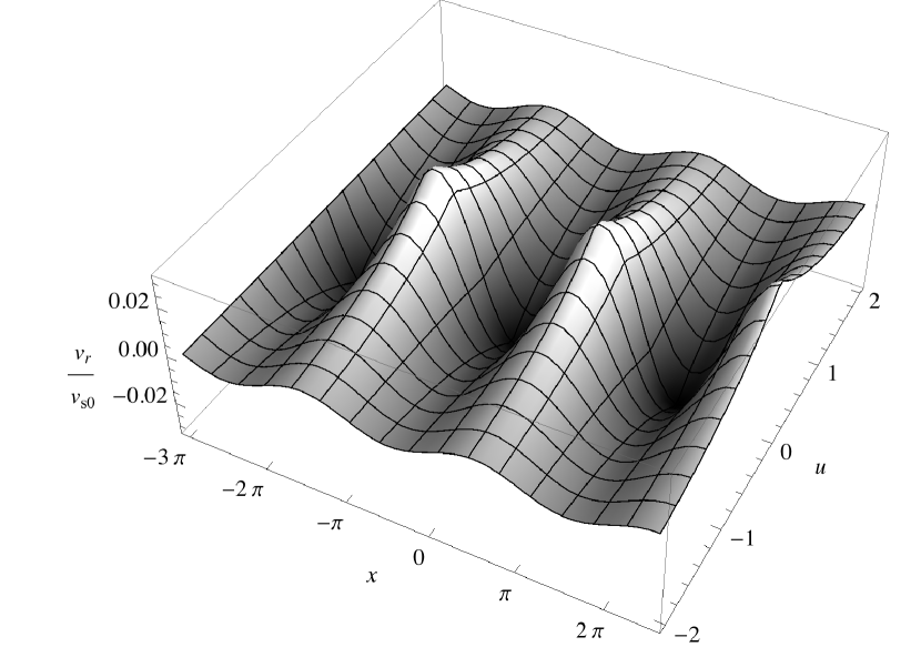
Figure 1. We plot the radial component of the velocity $v_{r}$ normalized to the constant sound velocity $v_{\mathrm{s}0}$ in correspondence to the value $\alpha=0.01,k_{0}H=5,\mathcal{A}=1$.

We see how the azimuthal equation completely fixes the disk profile at the zeroth order in $\epsilon_{z}$. The resulting accretion radial velocity has an oscillatory character along the radial coordinate around $r_{0}$, of the same kind found in Montani and Benini (2009). According with the discussion pursued in that work, this velocity profile is able to account for the local matter infall, but it does not clarify how the central object can receive this accretion rate. In fact the following expression for the accretion rate $\dot{M}_{\mathrm{S}}$ holds

(61) $$\frac{{\dot{M}_{\mathrm{S}}}}{\epsilon_{0}H^{2}v_{s0}}=\displaystyle\frac{8\pi}{3}\mathcal{A}\alpha\sqrt{\epsilon_{z}}(x+k_{0}r_{0})\sin x\,,$$

leading to the non zero average for $x\in[-\pi,\pi]$

(62) $$\left\langle\displaystyle\frac{\dot{M}_{\mathrm{S}}}{\epsilon_{0}H^{2}v_{s0}}\right\rangle=\displaystyle\frac{16\pi^{2}}{3}\mathcal{A}\alpha\sqrt{\epsilon_{z}}\,.$$

This behaviour is sketched in fig.2

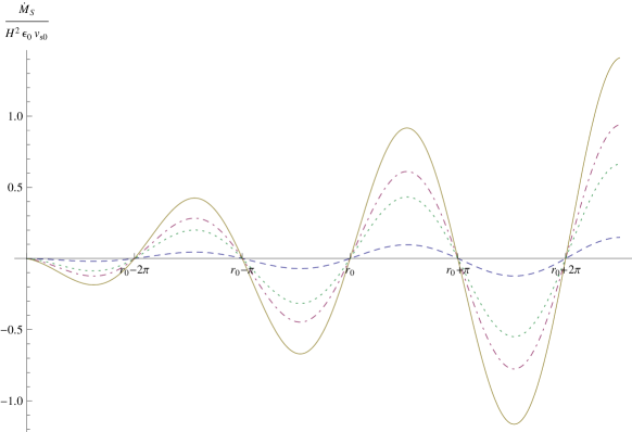
Figure 2. The behaviour of the accretion rate as a function of the radial coordinate is depicted. It is outlined how the material in-falling from outside in $r_{0}$ is greater than the lost one. The values of the parameters for the dotted, dot-dashed, dashed and thin curve are given by $\alpha=0.02,0.02,0.01,0.03$ and $\epsilon_{z}=0.005,0.01,0.001,0.01$ respectively.

The present analysis, differently from the linear case addressed in Montani and Benini (2009), lives in a full non-linear regime $Y\sim 1$ (i.e. $\mathcal{A}\sim 1$). Therefore we are able to identify the mass perturbation $\hat{\epsilon}$, as the relevant feature to deal with a global matter infall. Indeed, it seems that the non-linearity of the equilibrium configuration is not a strong enough feature to excite modes with non-zero radial averaged infall velocity.

Finally we observe how the vertical decay of the magnetic flux surface, over the equatorial plane, is slower in the present case with respect to the analysis pursued in Coppi (2005), as outlined in Fig3.

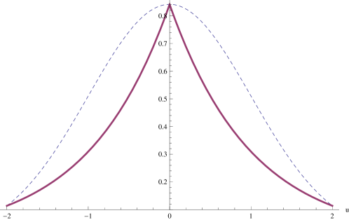
Figure 3. The vertical dependence of the disk profile $F(u^{2})$ is plotted in the present case (thin line) in comparison to the ideal MHD case (dashed line).

By other words, accounting for the azimuthal and electron force balance equations allows a higher intensity of the magnetic field in a given vertical region. The form of the total magnetic surfaces corresponds to the expression

(63) $$Y_{\mathrm{T}}(x,u^{2})=x+Y(x,u^{2})=x+\mathcal{A}\exp\left(-\sqrt{u^{2}}\right)\sin(x)\,.$$

Neglecting the toroidal component, which is regarded as small, the magnetic field components take the form

(64a) $$\frac{B_{r}}{B_{z0}}=-\displaystyle\sqrt{\epsilon_{z}}\partial_{u}Y_{\mathrm{T}}=\displaystyle\sqrt{\epsilon_{z}}\mathcal{A}\frac{u}{\sqrt{u^{2}}}\exp\left(-\sqrt{u^{2}}\right)\sin(x)\,,$$

(64b) $$\frac{B_{z}}{B_{z0}}=\partial_{x}Y_{\mathrm{T}}=1+\mathcal{A}\exp\left(-\sqrt{u^{2}}\right)\cos(x)\,,$$

The $\vec{B}$-field line are depicted in Fig.4.

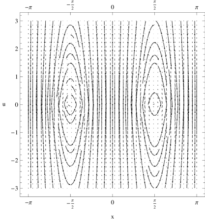
Figure 4. The magnetic field lines neglecting the toroidal components, in correspondence to the values $\mathcal{A}=1,\sqrt{\epsilon_{z}}=0.005$

6. Concluding Remarks

Our analysis constitutes a bridge scheme between the standard one-dimensional model for an accretion disk (Bisnovatyi-Kogan and Lovelace, 2001) and the reformulation provided in Coppi (2005) in terms of a local bidimensional MHD profile of the magnetically confined plasma. The original description relies on the setting of a viscoresistive MHD framework in which the angular momentum transport is allowed by the turbulent viscosity coefficient arising when the Reynolds number of the fluid has sufficiently high value. This paradigm has been able to provide with a satisfactory interpretation of some observed feature in strongly accreting system like X-ray binary pulsars.

On the other hand, the approach introduced in Coppi (2005) starts from a criticism concerning the possibility to generate in the plasma of the disk significant viscosity and resistivity effects. Therefore the disk morphology has been addressed on a purely theoretical point of view, relying on the hypotheses of the ideal bidimensional MHD in axial symmetry. However this point of view cannot properly account for the accretion mechanism because it stands only for a velocity field completely dominated by the Keplerian rotation. In fact, including radial and vertical velocity in this bidimensional MHD scheme requires a proper setting of the electron force balance equation.

We have constructed a scheme in which the viscoresistive bidimensional MHD scenario is implemented in the same spirit of Coppi (2005), but with the advantage to be able to account for the azimuthal and electron force balance equilibria, necessary to fix the accretion properties of the system. The resulting approach emerged as self consistent and, as far as a direct relation between the viscosity and the resistivity coefficients was addressed, we could fix the radial and vertical profile of the magnetic flux surfaces, due to the electromagnetic back-reaction. We devoted particular attention to the analysis of the linear case when the induced magnetic surface is a small correction only to the background features. Furthermore we solved the non-linear case in the limit of a vanishing ratio between the magnetic pressure to the thermostatic one.

The results we derived above constitute the first step for a reformulation of the mechanism at the ground of the accretion phenomenon in terms of local structures arising in the disk morphology, instead of the diffusive description characterizing the standard model.

This work was developed within the framework of the CGW Collaboration
(www.cgwcollaboration.it).

References

- Balbus and Hawley (1998) Balbus SA, Hawley JF (1998) Instability, turbulence, and enhanced transport in accretion disks. Rev Mod Phys 70:1, DOI 10.1103/RevModPhys.70.1
- Benini and Montani (2009) Benini R, Montani G (2009) 2-D MHD Configurations for Accretion Disks Around Magnetized Stars. ArXiv e-prints 0912.1721
- Bisnovatyi-Kogan and Lovelace (2001) Bisnovatyi-Kogan GS, Lovelace RVE (2001) Advective accretion disks and related problems including magnetic fields. New Astro Rev 45:663, DOI 10.1016/S1387-6473(01)00146-4
- Coppi (2005) Coppi B (2005) “crystal” magnetic structure in axisymmetric plasma accretion disks. Physics of Plasmas 12:7302, DOI 10.1063/1.1883667
- Coppi and Rousseau (2006) Coppi B, Rousseau F (2006) Plasma disks and rings with “high” magnetic energy densities. ApJ 641:458, DOI 10.1086/500315
- Ferraro (1937) Ferraro VCA (1937) The non-uniform rotation of the sun and its magnetic field. Mon Not R Astron Soc 97:458
- Lynden-Bell (1996) Lynden-Bell D (1996) Magnetic collimation by accretion discs of quasars and stars. Mon Not R Astron Soc 279:389
- Lynden-Bell and Pringle (1974) Lynden-Bell D, Pringle JE (1974) The evolution of viscous discs and the origin of the nebular variables. Mon Not R Astron Soc 168:603
- Montani and Benini (2009) Montani G, Benini R (2009) Linear Two-Dimensional MHD of Accretion Disks:. Crystalline Structure and Nernst Coefficient. Modern Physics Letters A 24:2667–2680, DOI 10.1142/S0217732309031879, 0909.0371
- Ogilvie (1997) Ogilvie GI (1997) The equilibrium of a differentially rotating disc containing a poloidal magnetic field. Mon Not R Astron Soc 288:63–77
- Pringle and Rees (1972) Pringle JE, Rees MJ (1972) Accretion disc models for compact x-ray sources. Astron Astrophys 21:1
- Ruffini and Wilson (1975) Ruffini R, Wilson JR (1975) Relativistic magnetohydrodynamical effects of plasma accreting into a black hole. Phys Rev D 12:2959–2962, DOI 10.1103/PhysRevD.12.2959
- Shakura (1973) Shakura NI (1973) Disk model of gas accretion on a relativistic star in a close binary system. Soviet Astronomy 16:756
- Spruit (2008) Spruit H (2008) Theory of magnetically powered jets. arXiv 0804:3096
- Velikhov (1959) Velikhov E (1959) Stability of an ideally conducting liquid flowing between cylinders rotating in a magnetic field. Sov Phys JETP 36(9):995–998
- Verbunt (1982) Verbunt F (1982) Accretion disks in stellar x-ray sources - a review of the basic theory of accretion disks and its problems. Space Science Reviews 32:379, DOI 10.1007/BF00177448