Neutrino Mass Sum-rules in Flavor Symmetry Models
Abstract
Four different neutrino mass sum-rules have been analyzed: these frequently arise in flavor symmetry models based on the groups , or , which are often constructed to generate tri-bimaximal mixing. In general, neutrino mass can be probed in three different ways, using beta decay, neutrino-less double beta decay and cosmology. The general relations between the corresponding three neutrino mass observables are well known. The sum-rules lead to relations between the observables that are different from the general case and therefore only certain regions in parameter space are allowed. Plots of the neutrino mass observables are given for the sum-rules, and analytical expressions for the observables are provided. The case of deviations from the exact sum-rules is also discussed, which can introduce new features. The sum-rules could be used to distinguish some of the many models in the literature, which all lead to the same neutrino oscillation results.
1 Introduction
The peculiar mixing scheme displayed by leptons has led to a keen interest in the field of flavor symmetries [1, 2]. In most cases, a model is constructed in order to reproduce the so-called tri-bimaximal mixing (TBM) pattern [3], defined by the following leptonic, or Pontecorvo-Maki-Nakagawa-Sakata (PMNS), mixing matrix
| (1) |
Here , , and contains the Majorana phases and . The latter are only manifest in lepton number violating processes, such as neutrino-less double beta decay (). It is rather noteworthy that the (in general) arbitrary mixing structure in displays, with good precision, such an aesthetic and symmetric form (TBM). This pattern is a very economic zeroth order description of lepton mixing [4]. As always, if a peculiar mixing is observed in Nature, one attributes this to the presence of a symmetry: in flavor physics this symmetry is called “flavor symmetry”. After choosing a group, one needs to know the irreducible representations and their well-defined multiplication rules. By identifying particles with the representations and demanding that the total Lagrangian is a singlet under the chosen symmetry group, the Yukawa couplings and hence the mixing matrices are constrained. However, even after choosing a symmetry group, there remains considerable freedom regarding the identification of the particle content with the irreducible representations of the group, the type and number of new particles introduced, and the way in which neutrino mass is generated. For instance, Ref. [5] contains a list of 52 models, all of which333The list in Ref. [5] is from March 2010, an updated version from July 2010 contains 61 models. are based on and all of which lead to TBM. The question then arises: how can these models be distinguished from one another? There are several approaches to this problem444Other, less scientific criteria are the simplicity or maybe even the “beauty” of the model.:
-
•
unavoidable corrections to the leading order mixing angle predictions may depend on the model details and may influence the mixing angles, if those are measured with sufficient precision;
-
•
lepton flavor violating processes such as and are often predicted by the model, and the branching ratios or relations between certain processes are characteristic features of a model;
-
•
sometimes the scalar sector of a model contains low mass states, which could leave their imprint on lepton flavor violation or in a modification of the scalar (Higgs) sector of the Standard Model;
-
•
sometimes the choice of the identification particle representation is incompatible with Grand Unification, a requirement which once imposed could be used to disregard some models or to only allow for models that can be accommodated in GUTs;
-
•
sometimes the necessary “VEV alignment” can only be achieved at the price of a severe amount of additional particle and formalism input;
-
•
one drawback of a model is when it cannot achieve successful leptogenesis, or can do so only with additional input.
In this work another property of flavor models is exploited, namely the frequent appearance of neutrino mass sum-rules. In particular, the relations
| (2) | ||||
| (3) | ||||
| (4) | ||||
| (5) |
which have been shown to emerge from several (∗), (#) and (†) models, will be carefully analyzed. In these four expressions the neutrino masses are understood to be complex, i.e., , and, in the standard parametrization given above, . Different relative signs between the masses play no role for the observables.
It is clear that no single method can be successful in distinguishing flavor models; rather one needs a combination of them. The aim of the present paper is to emphasize the possible role of the neutrino mass observables. The potential importance of neutrino mass sum-rules has been noted before in Refs. [28, 31, 16, 43, 5]. Here the intention is to stress this point further, and to provide a detailed, analytical and comparative analysis of four of the most frequently appearing sum-rules.
There are three different and complementary observables to test neutrino mass: beta decay, neutrino-less double beta decay, and cosmology. In the general case, i.e., without any relation between the neutrino masses, there are well-known relations between the corresponding measurable quantities, leading to certain allowed areas in the parameter spaces spanned by them. The consequence of a neutrino mass sum-rule is that the three observables do not fill the whole allowed parameter space anymore, but are limited to certain constrained regions. Plots which display these regions are provided, along with analytical results. Furthermore, “perturbed” sum-rules are investigated, i.e., where the expressions in Eqs. (2)–(5) are satisfied only approximately. Here new features can arise, for instance, the sum-rule can be realized in the inverted mass ordering once perturbations are applied, whereas the exactly satisfied sum-rule cannot.
In Section 2 there is a brief discussion of the structure of some of the models from which the sum-rules [Eqs. (2)–(5)] emerge. Section 3 contains a summary of the neutrino mass observables, as well as a description of the calculations required to obtain analytical results for the observables, when a sum-rule applies. Since this procedure is very similar for all sum-rules, a detailed analysis is presented for only one of them, with the results for the other sum-rules listed in several tables and plots. Section 4 deals with perturbed sum-rules; a summary and conclusion is given in Section 5.
2 Sum-rules in flavor symmetry models
Many flavor symmetry models have been constructed to explain neutrino masses and lepton mixing, and some of those models contain simple sum-rules between the light neutrino masses. The non-Abelian symmetries and have been widely used in the literature (see the reviews in Ref. [1, 2]). A common feature of all models is that “flavon fields” are introduced and assigned to certain representations of the symmetry group. Once the flavons obtain a vacuum expectation value (VEV) the symmetry is broken. Usually the VEVs are aligned in the sense that, e.g., for a triplet flavon the relation holds, and only with such a VEV alignment is the desired mixing scheme obtained. This alignment can either simply be assumed, or can explicitly be shown to correspond to a minimum of the full flavon potential, often at the expense of additional input.
The group contains one three-dimensional irreducible representation (IR) and three one-dimensional IRs , and . The fact that is the smallest discrete group containing a three-dimensional IR is the reason that it is the most frequently used group. In the most common models [8], the right-handed charged lepton singlets , and are identified as , ” and respectively, while the three lepton doublets are identified as . Two scalar triplets and of are introduced, as well as one scalar singlet . The necessary VEV alignment is and . With such a choice the final neutrino mass matrix produces TBM and obeys the sum-rule555Additional model details such as extra symmetries for the charged lepton mass hierarchy, or symmetries to separate the charged lepton and neutrino sectors, are not discussed here – the interested reader is referred to the original works.
Some other examples include Refs. [7, 8], where neutrino masses come from dimension-5 operators, or Ref. [6], where they originate from Higgs triplets in the type II seesaw mechanism. Note that this sum-rule can also be achieved with the symmetry [20], since is a subgroup of .
It is also possible to include additional flavon singlets transforming as and/or . However, with two singlets the only allowed combination is to have the singlet scalars transforming as and [14, 5]. Furthermore, TBM is only achieved when a rather strong assumption is made: the VEV of one singlet times a Yukawa coupling has to take the same value as the VEV of the other singlet times another coupling. If this is assumed [6, 14, 5], TBM is obtained and the neutrino masses exhibit the sum-rule
No sum-rule occurs when all three possible singlet flavons are introduced. In the context of models it is rather ad hoc to impose the above mentioned condition between the product of two a priori unrelated VEVs and couplings. However, a useful observation is that the group contains a two-dimensional IR . Roughly speaking, a scalar doublet transforming as under can take the role of the two singlets and , so that the necessary relation between their contributions occurs without additional input. This can be seen for instance in Ref. [24], where the above sum-rule is obtained with .
The models discussed above can be extended to include right-handed neutrinos and the type I seesaw mechanism. For instance, the model from Ref. [7] can be modified [8] by adding right-handed neutrinos transforming as , leading to an “inverted” sum-rule
Again, by replacing the singlet by two singlets , and assuming the same tuning between their VEVs and couplings as above, the sum-rule [5]
is found. Moreover, in seesaw models a scalar can take the role of the two singlets, so that the above sum-rule is found more naturally [41, 42].
The discussion above is just one example of how a sum-rule can arise. There are other cases, of course, but a model building discussion will not be entered into here. It is enough to state that each of the four sum-rules under discussion has been obtained in several , or models, and that this work focuses on these sum-rules. Note that the sum-rules occur in models which reproduce the TBM pattern; one could indeed find different sum-rules in models with different mixing patterns (e.g., Ref. [44]), or the same sum-rules in models leading to different mixing predictions. The results presented below are general enough to take the latter case into account.
3 Neutrino mass observables and sum-rules
3.1 General case
The three mass-dependent neutrino observables are: the sum of absolute neutrino masses (), the kinematic electron neutrino mass in beta decay () and the effective mass for neutrinoless double beta decay (). In terms of the “bare” physics parameters and , the observables are given by
| (6) |
| (7) |
| (8) |
The neutrino masses entering the above expressions are related to the smallest mass (normal ordering) or (inverted ordering) and to the measured solar and atmospheric mass-squared differences and by
| (9) |
for the normal and inverted ordering, respectively. Note that in this notation is always positive, and that the smallest mass will often be denoted as , which is equal to () in the normal (inverted) mass ordering.
Each neutrino mass observable is constrained by different experiments. The upper limit on from the Mainz and Troitsk experiments is 2.3 eV [45]; improvement by one order of magnitude is envisaged by the KATRIN experiment. Both and have current upper limits of around 1 eV. It is difficult to give a definite hard limit, due to uncertainties stemming from the nuclear physics () as well as the strong dependence of the cosmological neutrino mass limits on the data sets. For instance, Ref. [46] obtains an upper limit of 1.19 eV from the WMAP 7 year data set, while the addition of Baryon Acoustic Oscillations gives 0.85 eV. Fixing the Hubble parameter to the value obtained by the Hubble Space Telescopes gives 0.58 eV. Future probes such as the Planck experiment or gravitational lensing observations will go down to the 0.1 eV regime. The upper bound on the effective mass for neutrino-less double beta decay will also decrease to the 0.1 eV level in future experiments such as CUORE, GERDA, Majorana, SuperNEMO etc.
There is one caveat worth noting: the extraction of neutrino mass constraints from neutrino-less double beta decay implicitly assumes that neutrinos are Majorana particles, and that no other lepton number violating process besides light neutrino exchange contributes to this process. Furthermore, for the cosmological mass limits one needs to assume the validity of the standard CDM model. This discussion will not be entered into here, and the standard interpretations are assumed to be applicable.
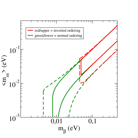
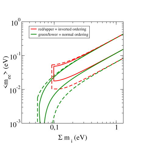
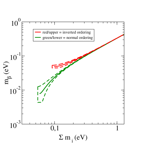
The relations between , and are well known [47], and allow one to plot one observable against another. This is shown, for the sake of completeness, in Fig. 1, where against , against and against is plotted, respectively. The best-fit values of the oscillation parameters, and their ranges (taken from Ref. [48], see Table 1) have been used. In the general case, i.e., without any assumptions about neutrino mass, the observables can lie at any allowed point in parameter space. If specific values for two or maybe even all three of the neutrino mass observables were determined experimentally, this would allow for a measurement of the neutrino mass hierarchy, the absolute neutrino mass scale, or maybe even one of the Majorana phases [49]. As mentioned before, this work will discuss the impact of neutrino mass sum-rules on the parameter space. For the sum-rules under discussion, only specific regions in parameter space are allowed, so that models containing these sum-rules could eventually be ruled out by future measurements.
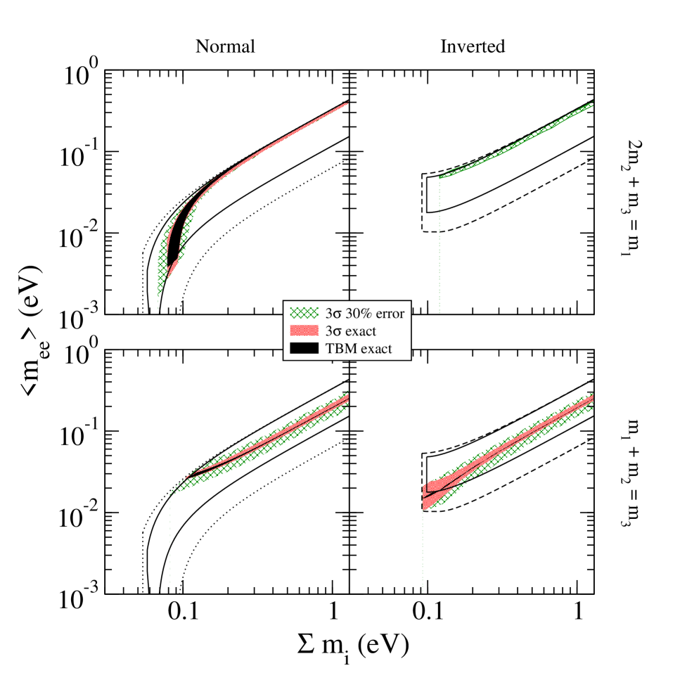
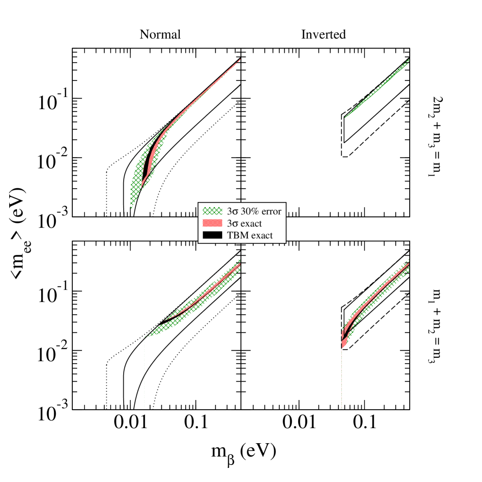
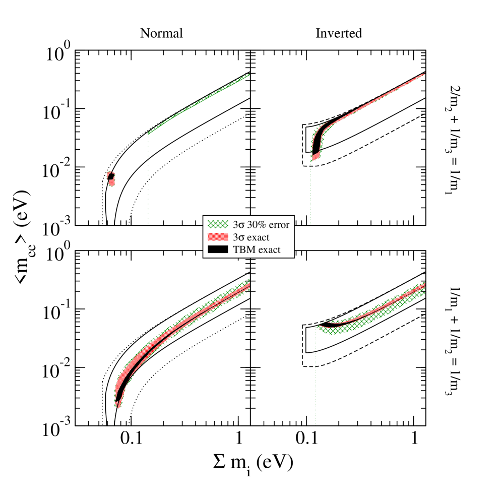
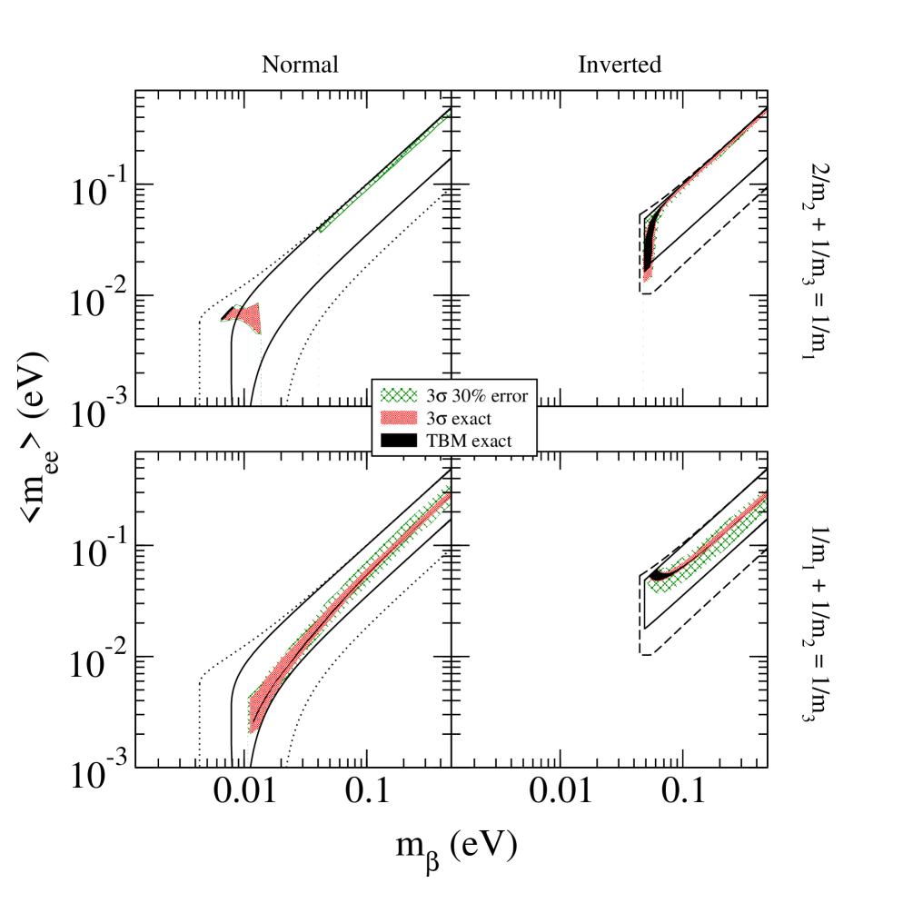
The main results of this work are presented in Figs. 2, 3, 4 and 5. They show the phenomenological consequences of the sum-rules for three cases: (i) “TBM exact”, denoting the exact sum-rules for TBM and the values of the mass-squared differences; (ii) “ exact” denoting the sum-rules for the current ranges of the oscillation parameters (see Table 1); (iii) “ 30 % error” denoting the sum-rules violated by 30 % (see Section 4 for an explanation of this) and the current ranges of the oscillation parameters. In addition, the numerical results in Tables 2, 3, 4 and 5 show the effect of different levels of perturbations on each of the observables.
The following section presents the calculation of analytical expressions for the observables, in the presence of the sum-rules under discussion.
3.2 Limits on mass observables
Starting with the sum-rule , the relation for the absolute values can be found. Using the expressions for the mass-squared differences in Eq. (9) for the normal ordering, this relation is solved for to obtain its lower limit:
| (10) |
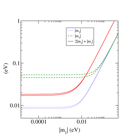
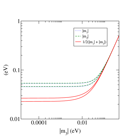
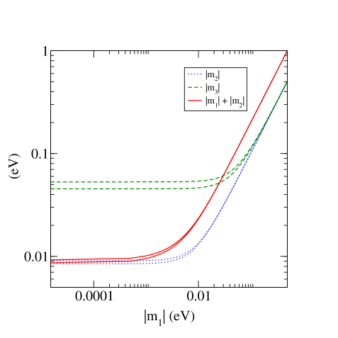
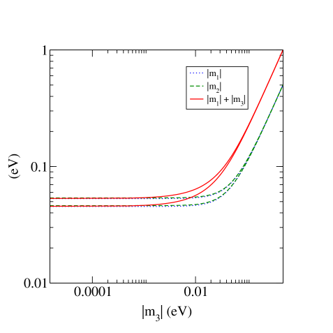
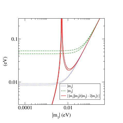
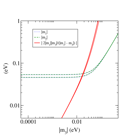
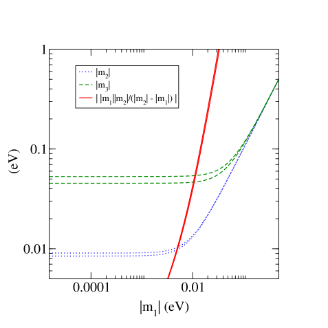
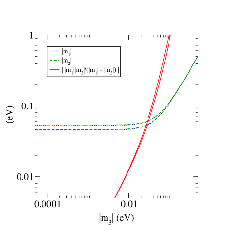
Here the exact result has been expanded in terms of small , and the mass-squared differences take their best-fit values for the numerical value. The same analysis can be performed for each of the sum-rules: the limits on the lightest masses in terms of the mass-squared differences and are shown in Table 6. A graphical representation is shown in Figs. 6, 7, 8 and 9. The individual (absolute) masses are calculated as a function of the smallest mass for the normal and inverted ordering, which gives the green and blue (dashed and dotted) curves. The sum-rules are used to obtain an upper limit for the heaviest mass, for instance for the sum-rule and the normal ordering. Inserting into this expression the individual (absolute) masses obtained from the mass-squared differences gives the red (solid) lines. It follows that the value of the smallest mass for which this red (solid) line (the heaviest possible mass predicted by the sum rule) intersects the green (dashed) line (the heaviest mass obtained from the mass-squared differences) is just the lower limit on the smallest neutrino mass for which the sum-rule can be fulfilled.
Two special features are notable: Figure 6(b) shows that it is impossible to accommodate the inverted ordering if the sum-rule is exactly satisfied, and Fig. 8(a) reveals that is only exactly true for a small range of the lightest mass. However, these restrictions change once the sum-rule is violated by a small amount (see Section 4).
The limits on naturally lead to limits on the actual mass observables. For and , one simply substitutes the limits in Table 6 into the most general expression: the resulting limits are shown in Tables 7 and 8, where TBM has been assumed for the calculation of .
Regarding the effective mass for , in the case of exact TBM it is given as
| (11) |
where is the phase between and . This relative phase between the complex neutrino mass eigenvalues can be determined for each sum-rule, making it possible to give limits on . For example, the sum-rule can be separated into real and imaginary parts,
giving a solution for in terms of , and . Substituting this into Eq. (11) gives
| (12) |
for the normal ordering, and inserting the limit on the lightest mass obtained above
(Table 6) results in limits on the effective mass, summarized in Table 9.
The values of the Majorana phases in the case of quasi-degenerate (QD) neutrinos can be obtained by trivial geometrical considerations: for instance, in the case of the three complex vectors , and must add to zero. Because of the quasi-degeneracy, have a common length , so that the only configuration in which the sum-rule condition can be achieved is the one shown in the left part of Fig. 10, hence and . The effective mass is in this case simply
| (13) |
independent of . The same expression is found for the sum-rule and QD neutrinos.
In the case of , the only possible configuration is the one in the right part of Fig. 10, corresponding to and , and thus
| (14) |
The same result is found for .
Finally, an interesting possibility is the vanishing of either the smallest mass or the effective mass. In the general case, the latter is only possible in the case of normal ordering, see Fig. 1, and corresponds to a zero entry in the element of the neutrino mass matrix in the charged lepton basis. However, none of the sum-rules under discussion allow for this, which is obvious from the values in Table 9. For instance, choosing with TBM and demanding that the effective mass vanishes [see Eq. (11)] gives the relations and . This leads to , which is too large ( should be close to 1/30).
Similarly, for the same sum-rule the requirement would give , and equivalent statements can be made for the other sum-rules and mass orderings: the smallest mass is always non-zero.
4 Perturbed sum-rules
The sum-rules studied above occur in neutrino mass models based on flavor symmetries. In general, deviations from the “zeroth order” model predictions are expected, be it from renormalization group running, VEV misalignment, higher order non-renormalizable terms etc. These effects will lead to deviations from the exact sum-rules, a possibility which is taken into account in the numerical strategy outlined below. For example, with the sum-rule and a normal ordering, the perturbations are parameterized as
| (15) |
where is an additional phase. The sum-rule is thus violated by times the (complex) heaviest mass, , defined as . In this example the three neutrino masses are defined as
| (16) | ||||
| (17) | ||||
| (18) |
where for each value of the lightest mass , the solar mass-squared difference is varied in its range, the three phases are varied between zero and , and one checks that the resulting atmospheric mass-squared difference lies in the correct range. An analogous procedure can be used for the inverted ordering, starting with the lightest mass . This technique can be repeated for the different sum-rules, with the heaviest mass defined using the sum-rule in each case.
Tables 2, 3, 4 and 5 show the effect these perturbations have on the limits for the lightest neutrino mass and the neutrino mass observables in each sum-rule. In general, increasing results in a decrease in the lower limit for , which means that the lower limits for each observable also decrease. The dashes in Table 3 indicate that, for and the inverted ordering, there is no lower limit on the lightest neutrino mass for , and it follows that the limits on all three neutrino mass observables do not change as increases. Note than in all cases except the sum-rule (Table 4), the sum-rules only give lower bounds on the observables.666It is evident from Fig. 8(a) that the sum-rule places both upper and lower limits on the lightest neutrino mass, and therefore on each of the observables, as seen in Table 4.
It is interesting to note that for the sum-rule , the inverted ordering is allowed once perturbations are applied. One can show that in order for the sum-rule to be valid for eV, the parameter must be greater than about 0.0022. With the sum-rule and normal ordering, the addition of perturbations leads to a new allowed region in the QD neutrino mass range, where eV as long as . These effects can be explained by examining Figs. 6(b) and 8(a): in both cases the red (solid) and green (dashed) lines representing the sum-rule and heaviest mass are basically parallel for the exact sum-rule and QD neutrinos. The added perturbations would essentially cause the red (solid) line to shift up and cross the green (dashed) line, giving a new allowed region for QD neutrinos.
The plots in Figs. 2 and 3 show the allowed regions in parameter space for the sum-rules and ; the plots in Figs. 4 and 5 show the allowed regions for the sum-rules and . Since the sum-rules only give lower bounds, the allowed regions in each plot could in principle extend to larger values of . However, this would conflict with the upper bound from cosmology [46], so that points above eV ( eV) are not shown. The effect of perturbations of order is shown in each case, and one can see the new allowed regions for the sum-rule , inverted ordering (top right panel of Figs. 2 and 3), and the sum-rule , normal ordering (top left panel of Figs. 4 and 5). In the latter case, the rather constrained prediction for the observables in the hierarchical region remains relatively unchanged with perturbations applied, but there is now a new allowed region in the QD mass range.
Although there are some regions in parameter space which can satisfy more than one sum-rule (for example, in the case of the normal ordering, the point (0.2 eV, 0.05 eV, 0.03 eV) is allowed for the sum-rules and ), a careful examination of the plots in Figs. 2, 3, 4 and 5 shows that there are no points in the three-dimensional parameter space satisfying all four sum-rules simultaneously, for a given mass ordering. One might expect there to be an overlap in the case of QD neutrinos, but the values of are clearly separated, as shown in Eqs. (13) and (14). As an example of the consequences of these results, note that if the upper limit of was found to be 0.03 eV with the inverted ordering, one could rule out the sum-rules and . On the other hand, if was measured to be 0.012 eV with the normal ordering, only the sum-rules , and would be allowed, the latter only with perturbations .
5 Conclusion
A phenomenological study of neutrino mass sum-rules has been presented, with an emphasis on the predictions for the mass-dependent observables , and . The sum-rules , , and , which frequently occur in models based on , and , have been analyzed analytically and numerically. Limits for the three observables are listed in each case. The effects of sum-rule perturbations are studied, and the plots in parameter space reveal the signatures of each sum-rule, in both the perturbed and unperturbed case. Perturbations were shown to introduce properties forbidden by the unperturbed case, for instance the inverted ordering for . The allowed parameter space is specified by each sum-rule, and may allow certain cases to be ruled out or the correct case to be identified. Since these sum-rules occur frequently in models with discrete flavor symmetries, one may apply the results of this analysis to any other model that exhibits one of the sum-rules, which might prove useful for neutrino model builders.
Nevertheless, the main point of the present work is to emphasize the importance of neutrino mass observables in the task of distinguishing (some of) the huge amount of proposed models leading to the peculiar mixing scheme of leptons. Though this will presumably only be possible with the help of other observables and criteria, important information can be provided by the three complementary neutrino mass observables.
Acknowledgments
This work was supported by the ERC under the Starting Grant MANITOP and by the DFG in the project RO 2516/4-1 as well as in the Transregio 27.
References
- [1] G. Altarelli and F. Feruglio, arXiv:1002.0211 [hep-ph].
- [2] H. Ishimori, T. Kobayashi, H. Ohki, H. Okada, Y. Shimizu and M. Tanimoto, arXiv:1003.3552 [hep-th].
- [3] P. F. Harrison and W. G. Scott, Phys. Lett. B 535, 163 (2002) [arXiv:hep-ph/0203209]; Z. Z. Xing, Phys. Lett. B 533, 85 (2002) [arXiv:hep-ph/0204049]; X. G. He and A. Zee, Phys. Lett. B 560, 87 (2003) [arXiv:hep-ph/0301092].
- [4] S. Pakvasa, W. Rodejohann and T. J. Weiler, Phys. Rev. Lett. 100, 111801 (2008) [arXiv:0711.0052 [hep-ph]].
- [5] J. Barry and W. Rodejohann, Phys. Rev. D 81 (2010) 093002 [arXiv:1003.2385 [hep-ph]].
- [6] E. Ma, Phys. Rev. D 70 (2004) 031901 [arXiv:hep-ph/0404199]; E. Ma, Phys. Rev. D 72 (2005) 037301 [arXiv:hep-ph/0505209].
- [7] G. Altarelli and F. Feruglio, Nucl. Phys. B 720 (2005) 64 [arXiv:hep-ph/0504165].
- [8] G. Altarelli and F. Feruglio, Nucl. Phys. B 741 (2006) 215 [arXiv:hep-ph/0512103].
- [9] G. Altarelli, F. Feruglio and Y. Lin, Nucl. Phys. B 775 (2007) 31 [arXiv:hep-ph/0610165].
- [10] E. Ma, Mod. Phys. Lett. A 21 (2006) 2931 [arXiv:hep-ph/0607190]; E. Ma, Mod. Phys. Lett. A 22 (2007) 101 [arXiv:hep-ph/0610342].
- [11] F. Bazzocchi, S. Kaneko and S. Morisi, JHEP 0803 (2008) 063 [arXiv:0707.3032 [hep-ph]].
- [12] F. Bazzocchi, S. Morisi and M. Picariello, Phys. Lett. B 659 (2008) 628 [arXiv:0710.2928 [hep-ph]].
- [13] M. Honda and M. Tanimoto, Prog. Theor. Phys. 119 (2008) 583 [arXiv:0801.0181 [hep-ph]].
- [14] B. Brahmachari, S. Choubey and M. Mitra, Phys. Rev. D 77 (2008) 073008 [Erratum-ibid. D 77 (2008) 119901] [arXiv:0801.3554 [hep-ph]].
- [15] Y. Lin, Nucl. Phys. B 813 (2009) 91 [arXiv:0804.2867 [hep-ph]].
- [16] M. C. Chen and S. F. King, JHEP 0906 (2009) 072 [arXiv:0903.0125 [hep-ph]].
- [17] E. Ma, arXiv:0908.3165 [hep-ph].
- [18] P. Ciafaloni, M. Picariello, A. Urbano and E. Torrente-Lujan, Phys. Rev. D 81 (2010) 016004 [arXiv:0909.2553 [hep-ph]].
- [19] T. Fukuyama, H. Sugiyama and K. Tsumura, arXiv:1005.5338 [hep-ph].
- [20] F. Bazzocchi and S. Morisi, Phys. Rev. D 80 (2009) 096005 [arXiv:0811.0345 [hep-ph]].
- [21] M. C. Chen and K. T. Mahanthappa, Phys. Lett. B 652 (2007) 34 [arXiv:0705.0714 [hep-ph]]; M. C. Chen and K. T. Mahanthappa, Phys. Lett. B 681 (2009) 444 [arXiv:0904.1721 [hep-ph]].
- [22] G. J. Ding, Phys. Rev. D 78 (2008) 036011 [arXiv:0803.2278 [hep-ph]].
- [23] M. C. Chen, K. T. Mahanthappa and F. Yu, Phys. Rev. D 81 (2010) 036004 [arXiv:0907.3963 [hep-ph]].
- [24] F. Bazzocchi, L. Merlo and S. Morisi, Nucl. Phys. B 816 (2009) 204 [arXiv:0901.2086 [hep-ph]].
- [25] K. S. Babu and X. G. He, arXiv:hep-ph/0507217.
- [26] X. G. He, Y. Y. Keum and R. R. Volkas, JHEP 0604 (2006) 039 [arXiv:hep-ph/0601001].
- [27] S. Morisi, M. Picariello and E. Torrente-Lujan, Phys. Rev. D 75 (2007) 075015 [arXiv:hep-ph/0702034].
- [28] G. Altarelli, F. Feruglio and C. Hagedorn, JHEP 0803 (2008) 052 [arXiv:0802.0090 [hep-ph]].
- [29] B. Adhikary and A. Ghosal, Phys. Rev. D 78 (2008) 073007 [arXiv:0803.3582 [hep-ph]].
- [30] C. Csaki, C. Delaunay, C. Grojean and Y. Grossman, JHEP 0810 (2008) 055 [arXiv:0806.0356 [hep-ph]].
- [31] G. Altarelli and D. Meloni, J. Phys. G 36 (2009) 085005 [arXiv:0905.0620 [hep-ph]].
- [32] Y. Lin, Nucl. Phys. B 824 (2010) 95 [arXiv:0905.3534 [hep-ph]].
- [33] C. Hagedorn, E. Molinaro and S. T. Petcov, JHEP 0909 (2009) 115 [arXiv:0908.0240 [hep-ph]].
- [34] T. J. Burrows and S. F. King, Nucl. Phys. B 835 (2010) 174 [arXiv:0909.1433 [hep-ph]].
- [35] J. Berger and Y. Grossman, JHEP 1002 (2010) 071 [arXiv:0910.4392 [hep-ph]].
- [36] G. J. Ding and J. F. Liu, JHEP 1005 (2010) 029 [arXiv:0911.4799 [hep-ph]].
- [37] M. Mitra, arXiv:0912.5291 [hep-ph].
- [38] F. del Aguila, A. Carmona and J. Santiago, arXiv:1001.5151 [hep-ph].
- [39] A. Kadosh and E. Pallante, arXiv:1004.0321 [hep-ph].
- [40] T. J. Burrows and S. F. King, arXiv:1007.2310 [hep-ph].
- [41] F. Bazzocchi, L. Merlo and S. Morisi, Phys. Rev. D 80 (2009) 053003 [arXiv:0902.2849 [hep-ph]].
- [42] G. J. Ding, arXiv:1006.4800 [hep-ph].
- [43] M. Hirsch, S. Morisi and J. W. F. Valle, Phys. Rev. D 78, 093007 (2008) [arXiv:0804.1521 [hep-ph]]; F. Bazzocchi, L. Merlo and S. Morisi, Phys. Rev. D 80, 053003 (2009) [arXiv:0902.2849 [hep-ph]]; S. Morisi, J. Phys. Conf. Ser. 203, 012060 (2010) [arXiv:0910.2542 [hep-ph]].
- [44] G. Altarelli, F. Feruglio and L. Merlo, JHEP 0905 (2009) 020 [arXiv:0903.1940 [hep-ph]].
- [45] C. Kraus et al., Eur. Phys. J. C 40, 447 (2005) [arXiv:hep-ex/0412056]; V. M. Lobashev, Nucl. Phys. A 719, 153 (2003).
- [46] S. Hannestad, A. Mirizzi, G. G. Raffelt and Y. Y. Y. Wong, arXiv:1004.0695 [astro-ph.CO].
- [47] See e.g., F. Feruglio, A. Strumia and F. Vissani, Nucl. Phys. B 637, 345 (2002) [Addendum-ibid. B 659, 359 (2003)] [arXiv:hep-ph/0201291]; M. Lindner, A. Merle and W. Rodejohann, Phys. Rev. D 73, 053005 (2006) [arXiv:hep-ph/0512143]; G. L. Fogli et al., Phys. Rev. D 75, 053001 (2007) [arXiv:hep-ph/0608060]; S. Pascoli and S. T. Petcov, Phys. Rev. D 77, 113003 (2008) [arXiv:0711.4993 [hep-ph]].
- [48] G. L. Fogli et al., Phys. Rev. D 78, 033010 (2008) [arXiv:0805.2517 [hep-ph]].
- [49] See e.g., S. Pascoli, S. T. Petcov and T. Schwetz, Nucl. Phys. B 734, 24 (2006) [arXiv:hep-ph/0505226]; S. Hannestad, arXiv:0710.1952 [hep-ph]; W. Maneschg, A. Merle and W. Rodejohann, Europhys. Lett. 85, 51002 (2009) [arXiv:0812.0479 [hep-ph]].
| Parameter | |||||
|---|---|---|---|---|---|
| best-fit | |||||
| range | |||||
| range | |||||
| range |
| (eV) | (eV) | (eV) | (eV) | |||||
|---|---|---|---|---|---|---|---|---|
| NO () | IO () | NO | IO | NO | IO | NO | IO | |
| (eV) | (eV) | (eV) | (eV) | |||||
|---|---|---|---|---|---|---|---|---|
| NO () | IO () | NO | IO | NO | IO | NO | IO | |
| – | ||||||||
| – | ||||||||
| – | ||||||||
| (eV) | (eV) | (eV) | (eV) | |||||
| NO () | IO () | NO | IO | NO | IO | NO | IO | |
| – | – | – | – | |||||
| – | – | – | – | |||||
| and | and | and | and | |||||
| – | – | – | – | |||||
| and | and | and | and | |||||
| – | – | – | – | |||||
| and | and | and | and | |||||
| (eV) | (eV) | (eV) | (eV) | |||||
|---|---|---|---|---|---|---|---|---|
| NO () | IO () | NO | IO | NO | IO | NO | IO | |
| Sum-rule | Limits on | |
|---|---|---|
| Normal | Inverted | |
| Sum-rule | Limits on | |
|---|---|---|
| Normal | Inverted | |
| Sum-rule | Limits on | |
|---|---|---|
| Normal | Inverted | |
| Sum-rule | Limits on | |
|---|---|---|
| Normal | Inverted | |
