Inexact Solves in Interpolatory Model Reduction111 This work was supported in part by the NSF through Grants DMS-0505971 and DMS- 0645347 222 Dedicated to Danny Sorensen on the occasion of his 65th birthday.
Abstract
We investigate the use of inexact solves for interpolatory model reduction and consider associated perturbation effects on the underlying model reduction problem. We give bounds on system perturbations induced by inexact solves and relate this to termination criteria for iterative solution methods. We show that when a Petrov-Galerkin framework is employed for the inexact solves, the associated reduced order model is an exact interpolatory model for a nearby full-order system; thus demonstrating backward stability. We also give evidence that for -optimal interpolation points, interpolatory model reduction is robust with respect to perturbations due to inexact solves. Finally, we demonstrate the effecitveness of direct use of inexact solves in optimal approximation. The result is an effective model reduction strategy that is applicable in realistically large-scale settings.
keywords:
Model reduction; system order reduction; tangential interpolation, iterative solves, Petrov-Galerkin1 Introduction
The simulation of dynamical systems constitutes a basic framework for the modeling and control of many complex phenomena of interest in science and industry. The need for ever greater model fidelity often leads to computational tasks that make unmanageably large demands on resources. Efficient model utilization becomes a critical consideration in such large-scale problem settings and motivates the development of strategies for model reduction.
We consider here linear time invariant multi-input/multi-output (MIMO) systems that have a state space form (in the Laplace transform domain) as
| (1) |
Here, and denote Laplace-transformed system inputs and outputs, respectively; represents the internal system state. We assume that and are analytic in the right half plane; and that is analytic and full rank throughout the right half plane. Solving for in terms of , we obtain
| (2) |
This representation of the transfer function,
| (3) |
we refer to as a generalized coprime realization. Standard first-order descriptor system realizations, with for constant matrices , , and evidently fit this pattern with , , and . However, many dynamical systems can be described more naturally with generalized coprime realizations. For example, a system that includes internal system delays as well as transmission/propagation delays in its input and output could be described with a model
| (4) |
for , and , and . Taking the Laplace transformation of (4) yields the transfer function
which has the form of (3). The form of (3) can accomodate greater generality than this, of course, including memory convolution involving higher derivatives, second and higher-order polynomial differential equations, systems described via integro-differential equations, and systems where state variables may be coupled through infinite dimensional subsystems (possibly modeling internal propagation or diffusion). See Table 1 for other examples and [6] for further discussion.
| Descriptor Systems | ( possibly singular) |
|---|---|
| Delay Systems | |
| Second Order Systems | |
| Weighted Systems |
In many applications, the state space dimension, , is too large for efficient system simulation and control computation, so the cases of interest for us here have state space dimension vastly larger than input and output dimensions: . See [19] for a recent collection of such benchmark problems.
The goal is to produce a reduced system that will have approximately the same response (output) as the original system for any given input . For a given reduced-order , we construct reduced order models through a Petrov-Galerkin approximation of (1): Select full rank matrices and . For any input, , the reduced system output, , is then defined (in the Laplace transform domain) as:
| (5) | ||||
| (6) |
which defines the reduced transfer function as,
| (7) |
where
| (8) |
2 Interpolatory Model Reduction
Interpolatory reduced order models are designed to exactly reproduce certain system response components that result from inputs having specified frequency content and growth. The approach has been described for standard first-order system realizations in [13, 2, 11, 3] and extended to generalized coprime realizations in [6]. We summarize the basic elements of this approach below.
A set of points and (nontrivial) direction vectors constitute left tangential interpolation data for the reduced model, , if
| (9) |
Likewise, , and associated directions , constitute right tangential interpolation data for the reduced model, , if
| (10) |
Given left and right tangential interpolating data, interpolatory model reduction may be implemented by first solving the linear systems:
| (11) |
| (12) |
We assume that the two point sets and each consist of distinct points and that the vectors and are linearly independent sets. These vectors constitute “primitive bases” for the subspaces and . Define the associated matrices:
| (13) | ||||
| (20) |
The reduced model, , as defined in (7) and (1) using and from (13) and (20), interpolates at the points and , in respective output directions and input directions ; that is, conditions (9) and (10) are satisfied. If for some then first order bitangential moments match as well:
Interpolation of higher order derivatives of can be accomplished with similar constructions as well; see [6, 3] and references therein.
For large-scale settings with millions of degrees of freedom, interpolatory model reduction has become the method of choice since it does not require dense matrix operations; the major computational cost lies in solving the (often sparse) linear systems in (11) and (12). This contrasts with Gramian-based model reduction approaches such as balanced truncation [25, 24], optimal Hankel norm approximation [12] and singular perturbation approximation [21] where large-scale Lyapunov equations need to be solved. Moreover, these computational advantages have been enhanced for standard first order state-space realizations by strategies for optimal selection of tangential interpolation data, see [16].
2.1 Inexact Interpolatory Model Reduction
The basic framework for interpolatory model reduction presumes that the key equations (11) and (12) may be solved exactly or nearly so, at least to an accuracy associated with machine precision. Direct solution methods, employing sparse factorization strategies, for example, are capable of handling systems of significantly large order. However since the need for ever greater modeling detail and fidelity can drive system order to the order of millions, the use of direct solvers for the linear systems (11) and (12) often becomes infeasible and iterative methods must be employed that terminate with possibly coarse approximate solutions to the linear systems. We consider and evaluate issues related to these approaches here.
Suppose and are linearly independent sets in and define
| (21) |
and will be viewed as approximate solutions to the linear systems (11) and (12) and accordingly we will refer to them as “inexact” solutions to (11) and (12). Nonetheless, unless otherwise stated, these vectors can be any arbitrarily chosen linearly independent vectors in .
Define residuals, and , corresponding to and , as
| (22) |
The deviations from the corresponding exact solutions are then
| (23) |
The resulting (inexact) basis matrices destined for use in a reduced order model are
| (24) | ||||
| (25) |
Define reduced order maps associated with these inexact bases:
| (26) |
together with the associated inexact reduced order transfer function
Notice that we are free to make any choice for bases for the subspaces, and , in defining ; no change in the definition of (26) is necessary. As a practical matter, it is generally prudent to choose well conditioned bases in computation.
3 Forward Error
3.1 Interpolation Error
Inexactness in the solution of the key linear systems (11) and (12) produces a computed reduced order transfer function, that no longer interpolates ; typically, the reduced order system response will no longer match any component of the full order system response at any of the complex frequencies and that have been specified. How much response error has been introduced at these points ?
The particular realization taken for a transfer function can create innate sensitivities to perturbations associated with that representation. Define perturbed transfer functions,
In discussing perurbations in system response caused by and at , it is natural to introduce the following quantities:
to be condition numbers of the transfer function response, by way of analogy to the condition number of algebraic linear systems. (Unless otherwise noted, norms will always refer to the Euclidean -norm for vectors or the naturally induced spectral norm for matrices). It is straightforward to show that these quantities measure the relative sensitivity of the system with respect to perturbations in and , respectively:
For values of such that and are nonsingular, define the matrix-valued functions,
| (27) |
Where defined, and are differentiable (indeed, analytic) with respect to , having derivatives that satisfy:
| (28) |
with equivalent expressions for and . We will make a series of observations about properties of and which will have immediately apparent parallels to properties for and .
Observe first that and so both and are skew projectors. These projectors are of interest because the pointwise error in the transfer function can be expressed as
Similarly,
and
The derivative of this last expression can be computed with the aid of (28) and observing :
| (29) | ||||
We introduce the following (-dependent) subspaces:
maps vectors in onto along and maps vectors in onto along .
Given two subspaces of , say and , we express the proximity of one to the other in terms of the angle between the subspaces, defined as
is the largest canonical angle between and a “closest” subspace of having dimension equal to . Notice that if then and if and only if . is asymmetrically defined with respect to and , however if then . If and denote orthogonal projectors onto and , respectively, then .
The spectral norm of a skew projector can be expressed in terms of the angle between its range and cokernel [27]. In particular,
| (30) | ||||
| (31) |
Theorem 3.1
Given the full-order model , interpolation points , and corresponding tangential directions, and , let the inexact interpolatory reduced model be constructed as defined in (21)-(26). The (tangential) interpolation error at and is
| (32) | ||||
| (33) |
If then,
| (34) |
and
| (35) |
with .
Proof: From (23), , which implies then that and , which may be rearranged to obtain
| (36) |
Let be the orthogonal projector taking onto One may directly verify that and
| (37) | ||||
Now suppose is an orthogonal projector onto . We have then that , so that and
Taking norms, we obtain an estimate yielding (32):
(33) is shown similarly, noting first that
| (38) |
Defining the orthogonal projector, , that takes onto one observes next so that
When , we have
leading then to two estimates:
and
These can be combined to yield (34).
The last inequality comes from using (29) with :
Then from (36), (38), and the Cauchy-Schwarz inequality
which yields the conclusion.
Consider the effect of solving (11) and (12) approximately with successively increasing levels of accuracy that force the residual norms to zero, and . The multiplicative behavior of the error bound (34) with respect to and contrasts with the additive behavior seen in (32) and (33) and suggests some potential benefit in using the same interpolation points for both left and right interpolation, i.e., choosing for . Note that this choice also forces convergent (bitangential) derivative interpolation as shown in (35). Indeed, choosing for is a necessary condition for forming -optimal interpolatory reduced order models for first-order descriptor realizations, as we discuss in §5 (see also [16]). Beyond this, there can be notable computational advantages in choosing , since the linear systems to be solved in (11) and (12) then have the same coefficient matrix; allowing one potentially to reuse factorizations and preconditioners.
Certain applications require the retention of structural properties such as symmetry in passing from to and one is compelled to choose (“one-sided” model reduction), so the vectors might not be approximate solutions to (11) in the usual sense. Nonetheless, the behavior of the interpolation error is still governed by (32) and (33). We explore this in the following numerical example.
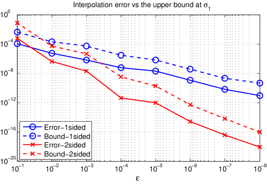
We illustrate the character of the results given in Theorem 3.1, bounding the response error at the nominal interpolation points caused by inexact solves in (11) and (12). To this end, we consider a delay differential equation of the form introduced in (4) taking , and . The coefficient matrices for the full order model in (4) were taken from [6]. We construct multiple reduced models all of order , solving (11) and (12) with different levels of accuracy. We chose three logarithmically spaced values, , and fixed them as interpolation points. We then obtained approximate solutions of varying accuracy to (11) and (12) in a manner described in more detail below, assembled the inexact interpolation basis matrices, and , and obtained reduced models of order having the same internal delay structure as the original system:
We considered both the usual “two-sided” model reduction process that involves approximate solution of both (11) and (12) and the “one-sided” process that involves approximate solutions only to (12) to generate and then assigning . Linear systems were solved with GMRES terminating with a final relative residual below a uniform tolerance denoted by .
We generated reduced order models in this way, varying the relative residual tolerance from down to . Figure 1 below shows the resulting interpolation errors and bounds from equations (32) and (34) for one-sided and two-sided cases, respectively, as varies. Observe that the bounds in Theorem 3.1 predict the convergence behavior of the true error quite well; the rates (slopes) are matched almost exactly. Note also that the interpolation error decays much faster for two-sided reduction than for one-sided reduction Indeed, the ratio of the two errors is close to , i.e., for a given tolerance , the interpolation error for two-sided reduction is approximately times smaller than the interpolation error for one-sided reduction.
Analogous results regarding behavior of the bounds and interpolation error are observed at and and so are omitted for brevity.
3.2 Global Error Bounds
Thus far we have focussed on the extent to which interpolation properties are lost in the computed reduced models when inexact solves are introduced into the process, considering in effect local error bounds. Clearly, it is important to understand the effect of inexact solves on the overall global quality of the reduced order model. There are two commonly used measures for closeness of two conforming dynamical systems (i.e., those with the same input and output dimensions):
Since reduced models are completely determined by the subspaces, and , as shown in (1), we first evaluate (in Theorem 3.2) how much inexact interpolatory subspaces, and , can deviate from the corresponding true subspaces, and , as a result of inexact solves. The effect of this deviation on the resulting model reduction (forward) error will be shown in Theorem 3.3. In this way, we are able to connect model reduction error to observable quantities that are associated with inexact solves, such as the relative stopping criterion .
Theorem 3.2
Let the columns of and be exact and approximate solutions to (12) and the columns of and be exact and approximate solutions to (11). Suppose approximate solutions are computed to a relative residual tolerance of , so that and , where the residuals and are defined in (22).
Denoting the associated subspaces as , , and then
| (39) | ||||
| (40) |
where and are diagonal scaling matrices defined as
and denotes the smallest singular value of the matrix .
Write with . Then
where is a diagonal matrix with positive diagonal entries, , that are fixed but for the moment unspecified.
Note that
Thus we have,
| (41) |
This bound is valid for any choice of diagonal scalings, , so we can minimize the right hand side of (41) with respect to . The Column Equilibration Theorem of van der Sluis [28] asserts that the optimal choice of is such that , independent of . If inexact solves terminate with residuals satisfying then we may take and to achieve the best bound possible with the information given. This leads to (39).
As a practical matter, the column scalings used in (39) and (40) will not be computationally feasible in realistic settings. If instead we scale the columns of and to have unit norm (cheap !) — taking and , the bound for (39) degrades to
where is the condition number of the linear system (12). A similar expression holds for . In many cases, these condition numbers have only modest magnitude and the bounds (39) and (40) remain descriptive.
Theorem 3.3
Proof: Note that for all for which and are both analytic,
So,
Maximizing over with gives
which leads immediately to the conclusion.
3.3 Illustrative examples
The process to be modeled arises in cooling within a rolling mill and is modeled as boundary control of a two dimensional heat equation. A finite element discretization results in a descriptor system of the form
where , , . For simplicity, we focus on a SISO full-order subsystem that relates the sixth input to the second output. For details regarding the modeling, discretization, optimal control design, and model reduction, see [8, 9].
We show the results of interpolatory model reduction using an ad hoc choice of interpolation points: logarithmically spaced points between and ; and an -optimal choice of interpolation points obtained by the method of [16]. For each case, we reduce the system order to using first exact interpolatory model reduction (i.e., the linear systems are solved directly) and then with inexact model reduction with varying choices of termination criteria. The resulting reduced-order models are denoted by and , respectively. To see the effect of the choice of interpolation points on the underlying model reduction problem, we vary the relative residual termination tolerance, between and and show how quickly converges to for both the ad hoc selection and the -optimal selection of interpolation points. Table 2 shows the relative error between and as decreases. For the -optimal choice of interpolation points, converges to as decreases, for the ad hoc choice of points, there is almost no improvement in accuracy until .
| -optimal | ad hoc | |
|---|---|---|
The behavior exhibited in Table 2 becomes clearer once we inspect the subspace angles between the exact interpolatory subspaces , and the inexact ones and . Table 3 shows the sine of the angle between the exact and inexact interpolatory subspaces as varies. While the gap decreases significantly as decreases for an -optimal selection of interpolation points, there is a much smaller improvement in the gap with respect to for an ad hoc choice of points. This behavior will be re-visited in more detail in §4.2 revealing that the -optimal (or good) interpolation points are expected to produce reduced order models that are more robust with respect to perturbations due to inexact solves.
| -optimal | ad hoc | -optimal | ad hoc | |
|---|---|---|---|---|
4 Backward error
Instead of seeking bounds on how much an inexactly computed reduced model differs from an exactly computed counterpart, one may view an inexactly computed reduced order model as an exactly computed reduced order model of a perturbed full order system. That is, we wish to find a full order system
| (42) |
so that the inexactly computed reduced model for would be an exactly computed interpolatory reduced model for . Given left and right tangential interpolation data as in (9) and (10) that has contributed toward producing the inexactly computed interpolatory reduced model , find as in (42) so that
and so that could have been computed from the perturbed system from the given tangential interpolation data via an exact computation. Specifically, given computed (inexact) projecting bases
as in (21), and a resulting (inexact) reduced order coprime realization
find a full-order system so that left and right interpolation conditions hold:
| (43) | ||||
| (44) |
and so that
| (45) |
There (typically) will be an infinite number of possible systems, , that are consistent with the computed reduced system in this sense — we are interested in those that are close to the original system with respect to a convenient system norm such as or . In order to proceed, it is convenient to restrict the class of backwardly compatible systems, . We consider those that have realizations that are constant perturbations from the corresponding original system factors:
| (46) |
where , , and are constant matrices. The conditions (43), (44), and (45) impose constraints on , , and . Indeed, (43) and (44) imply that
(45) implies that
Taken together, we find that backward perturbations of the form (46) can exist only if
| (47) |
Thus, we find constraints on the inexact interpolation residuals and in order for a backwardly compatible system of the form (46) to exist. More complicated perturbation classes than (46) may be considered that would allow us to remove the conditions (47), of course, but instead we choose to focus on a computational framework that guarantees (47). The Biconjugate Gradient Algorithm (BiCG) will be an example of an iterative solution strategy that fits this framework [1, 4]; others can be constructed without difficulty, although many standard strategies such as GMRES, do not fit this framework.
4.1 The Petrov-Galerkin Framework for Inexact Solves
We have observed above that (47) is necessary for there to be a well-defined backward error of the form (46) to exist. The simplest framework within which one may generate reduced order models that are guaranteed to satisfy this condition involves a Petrov-Galerkin formalism for producing approximate solutions to (11) and (12). For simplicity, we restrict our discussion to the case that (identical left and right interpolation points).
Let and be -dimensional subspaces of satisfying a nondegeneracy condition: for all shifts, to be considered. The Petrov-Galerkin framework for generating approximate solutions to the interpolation conditions (11) and (12) proceeds as follows:
| Find | ||||
| (48) |
Computed quantities generated within a Petrov-Galerkin framework will be denoted with a “tilde” to distinguish them from earlier “hat” quantities where no structure was assumed in the inexact solves. The following theorem asserts that if a reduced order model is computed within a Petrov-Galerkin framework (4.1), then one can obtain a structured backward error that throws the effect of inexact solves back onto a perturbation on the original dynamical system.
Theorem 4.1
Given a full order model , interpolation points , and tangent directions and , let the inexact solutions for and for be obtained in a Petrov-Galerkin framework as in (4.1). Let and denote the corresponding inexact interpolatory bases; i.e.
| (49) |
Define residuals
residual matrices
| (50) |
and the rank matrix
| (51) |
Let denote the computed inexact reduced model via the Petrov-Galerkin process where
| (52) |
Then, exactly tangentially interpolates the perturbed full-order model
| (53) |
at each :
| and |
Proof: The computed model, , will (exactly) tangentially interpolate a perturbed model provided the following interpolation conditions hold:
Equivalently, these can be interpreted as conditions on the perturbation . Rewriting this using notation defined above, must satisfy
| (54) |
The Petrov-Galerkin framework guarantees and . Substitution of from (51) into (54) verifies that is a perturbation to for which the computed (inexact) vectors become (exact) interpolation vectors.
Note that since ,
Consequently,
the reduced model
obtained by inexact solves in (52) is what one would have
obtained by exact interpolatory model reduction of .
Theorem 4.2
Proof: Note that
Let have an orthogonal factorization as with . Then
where we have introduced a diagonal scaling matrix
Easily one sees . For the remaining term, note that
A similar bound for is produced by an analogous process, which leads then to the final estimate for .
Note that the perturbation is completely determined by accessible, computed quantities. Hence, one can use to determine how accurately one must solve the underlying linear systems in order to assure system fidelity of a given order.
Theorem 4.3
If then
Proof: The system-wise backward error associated with inexact solves may be written as
Define and observe that
To estimate , a rearrangement of the definition of provides
So we have immediately,
Since , this last expression can be rearranged to obtain
which implies the conclusion.
By combining Theorem 3.3 with Theorem 3.2 or combining Theorem 4.2 with Theorem 4.3, we approach our goal of connecting quantities that we have control over, such as the termination threshold, , to relevant system theoretic errors, and , which are quantities we would like to control.
One may use these expressions as a basis to devise and investigate different, effective stopping criteria in large-scale numerical settings. For example, while appears explicitly in Theorem 3.2 in a way that suggests its use as a relative residual norm threshold; while Theorem 4.2 suggests a scaling of the residual norm by the norm of the solution vector as another possible stopping criterion. These and related ideas are the focus of on-going work.
4.2 Quantities of interest in derived bounds
By combining Theorem 4.2 with Theorem 4.3, one observes that perturbation effects of the inexact solves on the system theoretical (model reduction related) measures critically depend on the four quantities: The norm of the oblique projector of the underlying model reduction problem, reciprocals of the minimum singular values of the scaled primitive bases and ; and the stopping criterion for the inexact solves, (which affects and .)
The term is associated directly with inexact solves and is under the control of the user. The remaining quantities , and , depend largely on the selection of interpolation points and tangent directions, but the influence of interpolation data on the magnitude of these quantities is difficult to anticipate.
In this section, we will investigate experimentally the effects of the interpolation point selection on the three quantities of interest, , and , appearing in the derived bounds. These quantities are continuous with respect to the primitive basis vectors, and in neighborhoods where is nonsingular (i.e., where the projector is well defined). Thus it will be sufficient to examine how the magnitudes of the quantities of interest depend on interpolation data presuming that the necessary linear solves are done exactly; for modest convergence thresholds, the effect of inexact solves on these magnitudes is secondary to the effect of interpolation point location.
For our numerical study, we use the International Space Station 12A Module as the full-order model. The model has order . We examine a single-input single-output subsystem, , reducing the order from to order with varying from to in increments of two. For each reduced order, we chose random shift selections and computed , and . For each , shifts were sampled from a uniform distribution on a rectangular region in the positive half-plane: , where the and are taken over all the poles of the system. The remaining shifts were taken to be the complex conjugates of this random sample, so as to produce a shift configuration that was closed under conjugation. Additionally for each , we applied model reduction using the -optimal interpolation points generated by the method of [16]. Then, for each , out of the randomly generated shift selections, we counted the number of cases where the random shift selection yielded smaller values of , and . The results are shown in Figure 2. Figure 2-(a) and -(b) show that for most of the cases, the -optimal interpolation points yield smaller values for , . Indeed, for , the -optimal points produced smaller values in more than of the cases. Also, for the last three cases: , , and , the -optimal interpolation points always yielded smaller quantities. The results are even more dramatic for the projector norm, which is important in scaling the perturbation effects caused by inexact solves, see Theorem 4.2: Out of cases ( selections for each value), the -optimal interpolation point selection produced smaller condition numbers in all except instances: instances for , and instances for . These numerical results illustrate that -optimal interpolation points can be expected to yield smaller values for , and , and hence should produce reduced order models that are more robust with respect to perturbations.
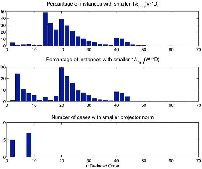
Figure 2 also shows that for , of the randomly selected shifts yielded smaller values of . However, when we inspected the randomly selected shift sets for in more detail, we observed some interesting additional features. We computed the three quantities , and for each of the randomly selected shift sets, and compared them with the corresponding value derived from an -optimal shift selection. The results are shown in Figure 3. The top plot shows where stands for the primitive interpolatory basis for the -optimal points. The bigger this ratio, the better the random shift selection. Even though for of the cases, the random selection was better, the highest this ratio becomes is , i.e., the random shifts were never much better than a factor of better than what -optimal shifts provided. For the remaining of the cases, the randomly selected shifts were worse, and often worse by a factor of or more. The situation for is shown in the middle plot. Once more, the situation is much more drastically in the favor of the -optimal interpolation points when the projector norm is inspected; the bottom plot in Figure 3 which depicts the ratio where denotes the projector for the -optimal points. As illustrated in Figure 2, there are no random shift cases yielding a smaller projector norm. Furthermore, in many cases the projector norm for the random shift selection is almost order of magnitudes higher than that of the -optimal points. Indeed, on average the projector norm for the random points is times higher. These numbers change more in the favor of the -optimal points as increases. For example, for , while the ratio becomes only as high as , it becomes as low as for some random selections; Also, the ratio 1 can reach as high as . For , for random selection is times higher than on average.
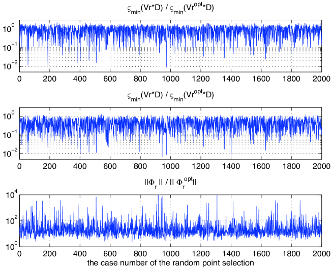
The three quantities we have been investigating appear to be extremely well conditioned for -optimal interpolation points. Even for , both , remain smaller than and is smaller than .
5 Inexact Solves in Optimal Interpolatory Approximation
The quality of the reduced-order model in interpolatory model reduction clearly depends on the selection of interpolation points and tangent directions. Until recently, this selection process was mostly ad hoc, and this factor had been the principal disadvantage of interpolatory model reduction. For systems in standard first-order state-space form, Gugercin et al. [16] have produced that an -optimal interpolation point / tangent direction selection strategy and proposed an Iterative Rational Krylov Algorithm (IRKA) to generate interpolatory reduced-order models that are (locally) optimal with respect to the norm. (An -optimal interpolation point selection strategy is still unknown for the general coprime factorization framework.) In this section, we investigate the behavior of inexact solves within the -optimal interpolatory approximation setting, specifically examining the behavior when inexact solves are employed in IRKA. In the rest of this section, we briefly review the optimal approximation problem and the method of [16]. We then show how inexact solves can be employed effectively in this setting and discuss observed effects on optimality of the final reduced model. Our discussion focuses on systems in first-order descriptor form:
| (55) |
where , and .
5.1 Optimal approximation problem
Given the full-order system as in (55), the goal of the optimal model reduction problem is to find a reduced-order model that minimizes the error; i.e.
| (56) |
Many researchers have worked on this problem. These efforts can be grouped into two categories: Lyapunov-based optimal methods such as [31, 26, 17, 18, 30, 32]; and interpolation-based optimal methods such as [23, 16, 15, 29, 10, 14, 20, 5, 7]. Here, we will focus on the interpolation-based approach. However we note that Gugercin et al. [16] has shown that these two frameworks are theoretically equivalent; hence motivating the use of interpolatory approaches to optimal approximation since they are numerically superior to the Lyapunov-based approaches.
Since the optimization problem (56) is nonconvex, obtaining a global minimizer is a hard task and can be intractable. The usual approach is to find reduced order models that satisfy first-order necessary optimality conditions. Meier and Luenberger [23] introduced interpolation-based -optimality conditions for SISO systems. Analogous -optimality conditions for MIMO systems have recently been developed by [16, 10, 29] which in turn have led to analogous algorithms for the MIMO case; see [16, 10] for more details.
Theorem 5.1
Given , let be the best order approximation of with respect to the norm. Then
| (a) | (57) | |||
5.1.1 An algorithm for interpolatory optimal model reduction
Theorem 5.1 reveals that any optimal reduced-order model is a bi-tangential Hermite interpolant to at mirror images of the reduced-order poles. However, since the interpolation points and the tangent directions (and consequently, and ), depend on the final reduced-model to be computed, they are not known a priori. The Iterative Rational Krylov Algorithm (IRKA) of [16] resolves this problem by iteratively correcting the interpolation points and the directions as outlined in Algorithm 1: The reduced-order order poles are reflected across the imaginary axis to become the next set of interpolation points; the tangent directions are corrected using residue directions from the current reduced model. Upon convergence, the resulting interpolatory reduced-order model satisfies the necessary conditions of Theorem 5.1. For further details on IRKA, see [16].
Algorithm 1
IRKA for MIMO Optimal Tangential Interpolation
-
1.
Make an initial -fold shift selection: and initial tangent directions and .
-
2.
. -
3.
while (not converged)
-
(a)
, , , and
-
(b)
Compute and where and are
the left and right eigenvector matrices for . -
(c)
for , and .
-
(d)
-
(e)
.
-
(a)
-
4.
, , ,
5.2 Inexact Iterative Rational Krylov Algorithm (InxIRKA)
For large system order, one may see from Algorithm 1, that the main cost of IRKA will generally be solving large linear systems at each step. If the IRKA iteration converges in steps, a total of linear systems will need to be solved. In settings where system dimension reaches into the millions, iterative linear system solvers become necessary and inexact linear system solves must be incorporated into IRKA. We refer to the modified algorithm as the Inexact Iterative Rational Krylov Algorithm (InxIRKA) and describe it in Algorithm 2 below. We employ the Petrov-Galerkin framework for the inexact solves. In Algorithm 2, the function in
denotes an inexact solve using a Petrov-Galerkin framework to approximately solve the linear systems and with initial guesses and , respectively, and a relative residual termination tolerance , i.e., at the end,
.
Algorithm 2
InxIRKA for MIMO Optimal Tangential Interpolation
-
1.
Make an initial -fold shift selection: and initial tangent directions and .
-
2.
for
-
3.
and .
-
4.
while (not converged)
-
(a)
, , , and
-
(b)
Compute and where and are the left and right eigenvector matrices of .
-
(c)
for , and
. -
(d)
for
-
(e)
and .
-
(a)
-
5.
, , , and
As discussed and illustrated in [16, 3], in most cases IRKA converges rapidly; that is, the interpolation points and directions at the step of IRKA stagnate rapidly with respect to . Let and denote the interpolation point and right-tangential direction, respectively, at the step. Then we expect that as increases, the solution of the linear system from the step approaches to the solution of the linear system at the step. This is precisely the reason that in Step of Algorithm 2, we use as an initial guess in solving at the . We expect that this initialization strategy will speed-up the convergence of the iterative solves.
The development of effective stopping criteria based rationally on system theoretic error measures as we have introduced them here is the focus of on-going work. Similar approaches toward the design of effective preconditioning techniques and reuse of preconditioners tailored for interpolatory model reduction and especially for optimal approximation are also under investigation.
5.3 Effect of Inexact Solves in the InxIRKA Setting
The first question to answer in InxIRKA is whether a statement can be made about the optimality as in the exact IRKA case. Employing the Petrov-Galerkin framework makes this possible:
Corollary 5.1
Corollary 5.1 shows that with the help of the underlying Petrov-Galerkin framework, we state that the final reduced model of InxIRKA is an optimal approximation to a nearby full-order model.
As we discussed in Section 4.2, for a good selection of interpolation points, interpolatory model reduction is expected to be robust with respect to perturbations due to inexact solves. Hence, if one feeds the optimal interpolation points from IRKA into an inexact interpolation framework, we expect that the resulting reduced model will be close to the optimal reduced model of IRKA. However, the optimal interpolation points are not known initially and InxIRKA will be initiated with a nonoptimal initial shift selection. If the initial interpolation points and directions are poorly selected, at the early stages of the iteration, perturbations due to inexact solves might be magnified by this poor selection. One can avoid this scenario by using a small termination threshold in the early steps of InxIRKA, and then gradually increase as the iteration starts to converge. However, we note that in our numerical experiments using random initialization strategies, InxIRKA performed robustly and yielded high fidelity reduced models that are also close to the true optimal reduced model. This is illustrated in §5.4 below. Effective initialization strategies are discussed in [16] as well.
5.4 Numerical results for InxIRKA
Here we illustrate the usage of inexact solves in the optimal approximation setting by comparing IRKA with InxIRKA. We use the example of §3.3, but with a finer discretization leading to a state-space dimension of . We focus on a MIMO version using -inputs and -outputs.
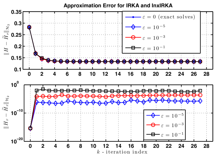
We reduce the order to using both IRKA and InxIRKA. In InxIRKA, the dual linear systems are solved in a Petrov-Galerkin framework using BiCG [4] where we use three different values for the relative residual termination threshold of : , , and . In all cases, the behavior of InxIRKA is virtually indistinguishable from that of IRKA. Starting with the same initial conditions, both IRKA and InxIRKA converge within iteration steps in all cases. The evolution of the errors and during the course of IRKA and InxIRKA, respectively, are depicted in the top plot of Figure 4. The figure shows that InxIRKA behavior is almost an exact replica of that of IRKA. The deviation from the exact IRKA is noticeable in the graph only for . To illustrate how much deviates from as IRKA and InxIRKA evolve, we show the progress of in the bottom plot of Figure 4. For this example, we initialized both IRKA and InxIRKA with an initial reduced-order model (as opposed to specifying initial interpolation points and tangent directions). Thus, initially and no linear solvers are involved in the first () step. One could expect that perturbation errors due to inexact solves might accumulate over the course of the InxIRKA iteration, but this does not appear to be the case as this figure illustrates. The magnitude of remains relatively constant throughout the iteration at a magnitude proportional to the termination criterion.
The resulting and model reduction errors, and (with obtained from IRKA), versus and (with obtained from InxIRKA) are given as varies in Table 4 below. The row corresponding to represents the errors due to exact IRKA.
| error | error | |
|---|---|---|
| 0 | ||
These numbers demonstrate that employing inexact solves in InxIRKA does not degrade the model reduction performance. We also measure the difference between and in both and norms as varies. These results are tabulated in Table 5:
Note that while and are respectively and , the contributions attributable to are much smaller in magnitude and do not alter the resulting (optimal) model reduction performance in any significant way. If one were to convert the perturbation errors in Table 5 to relative error (as opposed to the displayed absolute error), both and starts at for , and increases linearly by one order as increases by the same amount.
We finally list, in Table 6, the final exact and inexact optimal interpolation points due to IRKA, and InxIRKA for and :
Not surprizingly, the resulting interpolation points are very close to each other (though not the same). This can be viewed as another illustration of the fact that is an optimal approximation to a nearby full-order system.
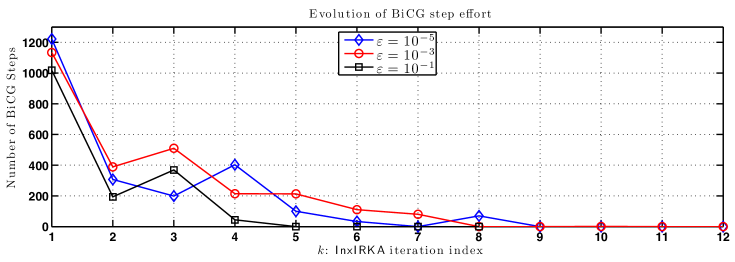
As discussed above, in the implementation of InxIRKA, we used the solution vectors from the previous step as the initial guess for the linear system in the next step taking advantage of the convergence in the interpolation points and tangent directions. To illustrate the effectiveness of this simple approach, throughout InxIRKA we monitor the number of BiCG steps required to solve each linear system. We illustrate the behavior only for one of the interpolation points. We choose the interpolation points closest to the imaginary axis since these produce the hardest linear systems to solve and invariably contribute most to the cost of inexact solves. Figure 5 depicts the the number of BiCG steps required as InxIRKA proceeds for these interpolation points using three different stopping criteria , and . The figure clearly illustrates that re-using the solutions from the previous steps works very effectively in reducing the overall cost of the BiCG. The number of BiCG steps goes from down to in to steps.
6 Structure-preserving interpolation for descriptor systems
The backward error analysis of §4 has been presented for the transfer functions in the generalized coprime factorization form as in (2). In this section, we show that stronger conclusions on the structure of the reduced system can be drawn in the case the system has a realization as a descriptor system, that is,
| (58) |
where , , and are constant matrices. In this case, for the interpolation points , and the tangent directions and , the associated primitive interpolatory bases and can be obtained from (13) and (20) using , (constant matrix) and (constant matrix). Then, the resulting reduced-order model is given by
| (59) |
where
| (60) |
Let the set denote given tangential interpolation data. Define the matrices and corresponding to the dynamical system and interpolation data :
| (61) |
| (62) |
is the Loewner matrix associated with the interpolation data and the dynamical system , is the shifted Loewner matrix associated with the interpolation data and the system , see [3, 22]. The next theorem presents a canonical structure for the exact interpolatory reduced-order model (59)-(60).
Theorem 6.1
6.1 The Petrov-Galerkin framework and structure preservation
Theorem 6.1 presents a canonical form for the exact bitangential Hermite interpolant in the case of standard state-space model. Next we show that if a Petrov-Galerkin framework is employed in the solution of the linear systems, the inexact reduced-model will have exactly the same form as the exact one. The result is a direct consequence of Theorems 4.1 and 6.1.
Corollary 6.1
Given the standard full-order model together with the the interpolation data , let the inexact solutions for and for be obtained in a Petrov-Galerkin framework as in (4.1). Let and denote the corresponding inexact Krylov bases as in (49). Define the residuals
Let the residual matrices and , and the rank matrix be as defined in (50) and (51), respectively. Then, the inexact interpolatory reduced-order model
| (64) |
is an exact Hermite bitangential interpolant for the perturbed full-order model
| (65) |
Morever, the reduced-order quantities satisfy
| (71) |
where and are the Loewner matrices associated with the dynamical systems and respectively, and the interpolation data as defined in (61) and (62).
Corollary 6.1 reveals that the inexact reduced-order model quantities have exactly the same structure as their exact counterparts. The interpolation data is the same in both cases; the only difference is that is replaced by in the construction that yields the Loewner-matrix structure. The preservation of this structure is independent of the accuracy to which the linear systems are solved. In the case where , the structure of the exact and inexact reduced-models becomes even simpler:
Corollary 6.2
Corollary 6.2 illustrates that in the case of , both of the reduced system matrices, and , are perturbations of rank to the diagonal matrix of interpolation points, .
References
- [1] Kapil Ahuja. Recycling Bi-Lanczos algorithms: BiCG, CGS, BiCGSTAB. Master’s thesis, Virginia Tech, Blacksburg, Virginia, August 2009.
- [2] A.C. Antoulas. Approximation of Large-Scale Dynamical Systems (Advances in Design and Control). Society for Industrial and Applied Mathematics Philadelphia, PA, USA, 2005.
- [3] A.C. Antoulas, C.A. Beattie, and S. Gugercin. Interpolatory model reduction of large-scale dynamical systems. In J. Mohammadpour and K. Grigoriadis, editors, Efficient Modeling and Control of Large-Scale Systems. Springer-Verlag, 2010.
- [4] R. Barrett, M. Berry, T.F. Chan, J. Demmel, J.M. Donato, J. Dongarra, V. Eijkhout, R. Pozo, C. Romine, and H. Van der Vorst. Templates for the Solution of Linear Systems: Building Blocks for Iterative Methods. Society for Industrial Mathematics, 1994.
- [5] C.A. Beattie and S. Gugercin. Krylov-based minimization for optimal model reduction. 46th IEEE Conference on Decision and Control, pages 4385–4390, Dec. 2007.
- [6] C.A. Beattie and S. Gugercin. Interpolatory projection methods for structure-preserving model reduction. Systems & Control Letters, 58(3):225–232, 2009.
- [7] C.A. Beattie and S. Gugercin. A trust region method for optimal model reduction. 48th IEEE Conference on Decision and Control, Dec. 2009.
- [8] P. Benner. Solving large-scale control problems. Control Systems Magazine, IEEE, 24(1):44–59, 2004.
- [9] P. Benner and J. Saak. Efficient numerical solution of the LQR-problem for the heat equation. Proc. Appl. Math. Mech, 4(1):648–649, 2004.
- [10] A. Bunse-Gerstner, D. Kubalinska, G. Vossen, and D. Wilczek. -optimal model reduction for large scale discrete dynamical MIMO systems. Journal of Computational and Applied Mathematics, 2009. doi:10.1016/j.cam.2008.12.029.
- [11] K. Gallivan, A. Vandendorpe, and P. Van Dooren. Model reduction via truncation: an interpolation point of view. Linear Algebra and Its Applications, 375:115–134, 2003.
- [12] K. Glover. All optimal Hankel-norm approximations of linear multivariable systems and their -error bounds. International Journal of Control, 39(6):1115–1193, 1984.
- [13] E. Grimme. Krylov Projection Methods for Model Reduction. PhD thesis, Coordinated-Science Laboratory, University of Illinois at Urbana-Champaign, 1997.
- [14] S. Gugercin. An iterative rational Krylov algorithm (IRKA) for optimal model reduction. In Householder Symposium XVI, Seven Springs Mountain Resort, PA, USA, May 2005.
- [15] S. Gugercin, A.C. Antoulas, and C.A. Beattie. A rational Krylov iteration for optimal model reduction. In Proceedings of MTNS, volume 2006, 2006.
- [16] S. Gugercin, A.C. Antoulas, and C.A. Beattie. model reduction for large-scale linear dynamical systems. SIAM Journal on Matrix Analysis and Applications, 30(2):609–638, 2008.
- [17] Y. Halevi. Frequency weighted model reduction via optimal projection. Automatic Control, IEEE Transactions on, 37(10):1537–1542, 1992.
- [18] D. Hyland and D. Bernstein. The optimal projection equations for model reduction and the relationships among the methods of Wilson, Skelton, and Moore. Automatic Control, IEEE Transactions on, 30(12):1201–1211, 1985.
- [19] J.G. Korvink and E.B. Rudnyi. Oberwolfach benchmark collection. In Dimension reduction of large-scale systems: proceedings of a workshop held in Oberwolfach, Germany, October 19-25, 2003, page 311. Springer Verlag, 2005.
- [20] D. Kubalinska, A. Bunse-Gerstner, G. Vossen, and D. Wilczek. -optimal interpolation based model reduction for large-scale systems. In Proceedings of the International Conference on System Science, Poland, 2007.
- [21] Y. Liu and B.D.O. Anderson. Singular perturbation approximation of balanced systems. International Journal of Control, 50(4):1379–1405, 1989.
- [22] A.J. Mayo and A.C. Antoulas. A framework for the solution of the generalized realization problem. Linear Algebra and Its Applications, 425(2-3):634–662, 2007.
- [23] L. Meier III and D. Luenberger. Approximation of linear constant systems. Automatic Control, IEEE Transactions on, 12(5):585–588, 1967.
- [24] B. Moore. Principal component analysis in linear systems: Controllability, observability, and model reduction. Automatic Control, IEEE Transactions on, 26(1):17–32, 1981.
- [25] C. Mullis and R. Roberts. Synthesis of minimum roundoff noise fixed point digital filters. Circuits and Systems, IEEE Transactions on, 23(9):551–562, 1976.
- [26] J.T. Spanos, M.H. Milman, and D.L. Mingori. A new algorithm for optimal model reduction. Automatica (Journal of IFAC), 28(5):897–909, 1992.
- [27] D.B. Szyld. The many proofs of an identity on the norm of oblique projections. Numerical Algorithms, 42(3):309–323, 2006.
- [28] A. van der Sluis. Condition numbers and equilibration of matrices. Numerische Mathematik, 14(1):14–23, 1969.
- [29] P. van Dooren, K.A. Gallivan, and P.A. Absil. -optimal model reduction of MIMO systems. Applied Mathematics Letters, 2008.
- [30] DA Wilson. Optimum solution of model-reduction problem. Proc. IEE, 117(6):1161–1165, 1970.
- [31] W.Y. Yan and J. Lam. An approximate approach to optimal model reduction. Automatic Control, IEEE Transactions on, 44(7):1341–1358, 1999.
- [32] D. Zigic, LT Watson, and C. Beattie. Contragredient transformations applied to the optimal projection equations. Linear Algebra and Its Applications, 188:665–676, 1993.