Nonlinear time series anaysis of the light curves from the black hole system GRS1915+105

Abstract

GRS 1915+105 is a prominent black hole system exhibiting variability over a wide range of time scales and its observed light curves have been classified into 12 temporal states. Here we undertake a complete analysis of these light curves from all the states using various quantifiers from nonlinear time series analysis, such as, the correlation dimension ($D_{2}$), the correlation entropy ($K_{2}$), singular value decomposition (SVD)and the multifractal spectrum ($f(\alpha)$ spectrum). An important aspect of our analysis is that, for estimating these quantifiers, we use algorithmic schemes which we have proposed recently and tested successfully on synthetic as well as practical time series from various fields. Though the schemes are based on the conventional delay embedding technique, they are automated so that the above quantitative measures can be computed using conditions prescribed by the algorithm and without any intermediate subjective analysis. We show that nearly half of the 12 temporal states exhibit deviation from randomness and their complex temporal behavior could be approximated by a few (3 or 4) coupled ordinary nonlinear differential equations. These results could be important for a better understanding of the processes that generate the light curves and hence for modelling the temporal behavior of such complex systems. To our knowledge, this is the first complete analysis of an astrophysical object (let alone a black hole system) using various techniques from nonlinear dynamics.

1 Introduction

Most of the systems in Nature are described by models which are inherently nonlinear. Since the discovery of deterministic chaos a few decades back and the development of various techniques in subsequent years, there remained the exciting prospect of a better understanding of the complex behavior shown by various natural systems in terms of simple nonlinear models. Evidence for low dimensional chaos has been reported - and disputed - not only in physical sciences, but also in many other fields such as, physiology, economics and social sciences (Schreiber, 1999). Particular attention has been paid to systems producing strange and chaotic attractors, the word strange refering to metric properties such as fractal dimension and the word chaotic representing dynamic properties like exponential divergence of nearby trajectories in phase space. A large number of techniques and measures from nonlinear dynamics and chaos theory are routinely being employed for the analysis of such systems. Excellent text books are now available that give a background knowledge on various methods in nonlinear dynamics (Hilborn, 1994; Sprott, 2003; Lakshmanan & Rajasekar, 2003).

One major difficulty in the analysis of real world systems is that our knowledge regarding the system is usually limited to a single scalar variable recorded as a function of time, called the time series. Therefore, a great deal of effort has been devoted to the characterisation of underlying attractors reconstructed from time series. The large number of techniques and computational schemes used for this purpose have been discussed in detail by many authors (Kantz & Schreiber, 1997; Aberbanel, 1996; Hegger et al., 1999).

Among the most important quantifiers used for the analysis of time series data are the correlation dimension ($D_{2}$), the correlation entropy ($K_{2}$) and the multifractal spectrum. Correlation dimension is often used as a discriminating statistic for hypothesis testing to detect nontrivial structures in the time series. But when the time series involves colored noise, a better discriminating measure is considered to be $K_{2}$ (Kennel & Isabelle, 1992). Finally, a complete characterisation of the underlying chaotic attractor is done using the generalised dimensions $D_{q}$ and the $f(\alpha)$ spectrum.

We have recently proposed automated algorithmic schemes (Harikrishnan et al., 2006, 2009a) for the computation of $D_{2}$ and $K_{2}$ from time series based on the delay embedding technique and applied it successfully to various types of time series data including that from standard chaotic systems, data added with white and colored noise and practcal time series like EEG and ECG. A generalisation of these schemes to compute the multifractal spectrum of a chaotic attractor has also been proposed (Harikrishnan et al., 2010, 2009b). These schemes provide a nonsubjective approach for the characterisation of strange attractors inherent in time series.

It should be noted that so far, most of the analysis of the light curves from X-ray binaries and active galactic nuclei (AGN) have used the conventional techniques such as the power spectrum and distribution. It is widely believed that the light intensity variations are mostly stochastic in nature. For example, it has been shown in the case of the most prominent black hole system, Cygnus X-1, that the observed light curves, at least in certain time scales, are consistent with some static nonlinear transformatons of stochastic variations in intensity (Uttley et al., 2005). The authors argue that models based on nonlinear dynamics are not required to explain the data.

But there are also some analysis based on nonlinearity measures that have been attempted earlier (Voges et al., 1987; Norris & Matilsky, 1989; Timmer et al., 2000) on the light curves of some prominent black hole systems, such as, Her X-1 and Cygnus X-1. But these studies have so far not been able to provide conclusive evidence for nontrivial structures in the temporal behavior of such systems. One reason for this has been the limited number of data sets available from such sources with sufficient signal to noise ratio required for such analysis (Norris & Matilsky, 1989). The scenario has changed in the last few years as enough data are now available through RXTE observations. Recently, a nonlinear time series analysis performed on light intensity data from the white dwarf variable PG1351+489 has enabled much more information regarding the system compared to the conventional power spectrum analysis (Jevtic et al., 2005) and attempts have been made to use these analysis to differentiate between neutron stars and black holes (Karak et al., 2010)

Studies on GRS1915+105 have been limited because it became active only over a decade ago. But the system turns out to be unique among all such sources in that it seems to flip from one state to another continuously with each state having its own temporal variability different from the other states. The light curves have been classified into 12 spectroscopic classes based on RXTE observations by Belloni et al. (2000). The nature of the light curves changes completely as the system flips from one state to another. Evidently, pure stochastic processes cannot account for such qualitative changes in the light curves. Hence the question naturally arises whether some nonlinear deterministic processes are also involved. We do find evidence to support this.

In this paper, we apply the above mentioned automated schemes developed by us to undertake a complete analysis of the X-ray light curves from GRS1915+105. Earlier, a surrogate analysis with $D_{2}$ as the discriminating measure has shown that a few of these states manifest the time evolutions analogous to that from low dimensional nonlinear systems with some inherent noise (Misra et al., 2006). This motivates us to undertake an exhaustive numerical analysis of the light curves from the source in all its temporal states using the prominent tools from nonlinear dynamics.

Another motivation for the present investigation has been derived from the fact that the accretion disk in such systems are driven by magneto-hydrodynamic turbulence which is an intrinsically non-linear process. A model for such a process should be nonlinear and is expected to show qualitative changes in its behavior as a control parameter is varied. For the X-ray radiation from an accretion disk, the rate of mass accretion could possibly be considered as a suitable control parameter. There also exists theoretical models to this effect (Voges et al., 1987; Atmanspacher et al., 1989a) from which it is possible to derive the temporal variability of the X-ray radiation in different regimes of mass accretion rate. Since many of the states of the black hole system under study show nonlinear character, a complete analysis of the light curves using various nonlinear measures can greatly help in the search for a nonlinear deterministic model to describe the temporal variability of the system.

Our paper is organised as follows: All the quantitative measures used in this paper and the corresponding computational schemes are discussed in detail in the following section. While §2.1 and §2.2 present the computational details for $D_{2}$ and $K_{2}$, §2.3 and 2.4 are concerned with SVD and $f(\alpha)$ spectrum respectively. The time series from a standard chaotic system - the Rossler system - is used as an example to illustrate the results in all the cases. The analysis of the X-ray light curves from the black hole system is then undertaken in §3 and the conclusions are drawn in §4.

Figure 1: The $D_{2}$ values of the Rossler attractor (with error bar), as a function of $M$ along with the $D_{2}$ values of $20$ surrogates (dashed lines). All computations are done with $10000$ data points.

2 Quantitative Measures used for the Analysis

2.1 Correlation dimension and surrogate analysis

Correlation dimension $D_{2}$ is often used as a discriminating statistic for hypothesis testing. The conventional method for the calculation of $D_{2}$ is the delay embedding method first introduced by Takens (1981), and used effectively by Grassberger & Procaccia (1983), now known as the GP algorithm. More details can be found in Sauer et al. (1991). It creats an embedding space of dimension $M$ with delay vectors constructed by splitting a discretely sampled scalar time series $s(t_{i})$ with delay time $\tau$ as

$$\vec{x_{i}}=[s(t_{i}),s(t_{i}+\tau),....,s(t_{i}+(M-1)\tau)]$$ (1)

The correlation sum is the relative number of points within a distance R from a particular ($i^{th}$) data point,

$$p_{i}(R)=\lim_{N_{v}\rightarrow\infty}{1\over N_{v}}\sum_{j=1,j\neq i}^{N_{v}}H(R-|\vec{x_{i}}-\vec{x_{j}}|)$$ (2)

where $N_{v}$ is the total number of reconstructed vectors and $H$ is the Heaviside step function. Averaging this quantity over $N_{c}$ randomly selected $\vec{x_{i}}$ or centers gives the correlation function

$$C_{M}(R)={1\over N_{c}}\sum_{i}^{N_{c}}p_{i}(R)$$ (3)

The correlation dimension $D_{2}(M)$ is then defined to be,

$$D_{2}\equiv\lim_{R\rightarrow 0}d({log}C_{M}(R))/d({log}(R))$$ (4)

which is the scaling index of the variation of $C_{M}(R)$ with $R$ as $R\rightarrow 0$. In pratice, a linear part in the $logC_{M}(R)$ versus $logR$ plot is identified subjectively, called the scaling region, and its slope is taken as $D_{2}$. But in our computational scheme, this is done algorithmically as discussed in detail elsewhere ( Harikrishnan et al. (2006)) and the scheme computes $D_{2}$ with error bar as a function of $M$. The scheme has also been shown to be suitable for hypothesis testing using surrogate data.

Figure 2: The upper panel shows the $D_{2}$ values of pure colored noise with spectral index $s=1.5$ as a function of $M$ along with surrogates. The lower panel shows the same for $s=2.0$.

Figure 3: The figure shows the $D_{2}$ values as a function of $M$ for the Rossler attractor data added with $50\%$ white noise ($s=0.0$) and the same percentage of colored noise ($s=2.0$) along with their respective surrogates. Note that, in the case of colored noise contamination (lower panel), the data values are still below that of the surrogates.

The rationale behind surrogate analysis is to formulate a null hypothesis that the data has been generated by a stationary linear stochastic process, and then attempt to reject it by comparing a suitable measure for the data with appropriate realisations of surrogate data. The method for the generation of surrogate data was originally proposed by Theiler and coworkers (Theiler et al., 1992) with the Amplitude Adjusted Fourier Transform (AAFT) algorithm. But Schreiber & Schmitz (1996, 2000) have proposed another iterative scheme, known as IAAFT scheme, which is similar but reported to be more consistent in representing null hypothesis (Kugiumtzis, 1999) for a wide class of stochastic processes. In this work, we apply this scheme to generate surrogate data sets using the TISEAN package (Hegger et al., 1999).

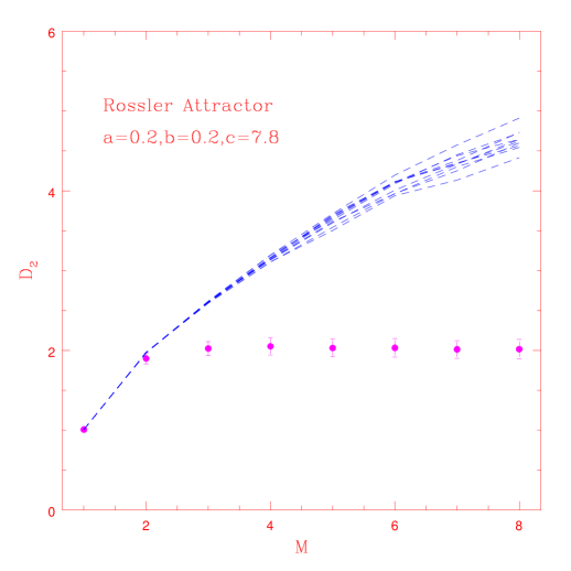
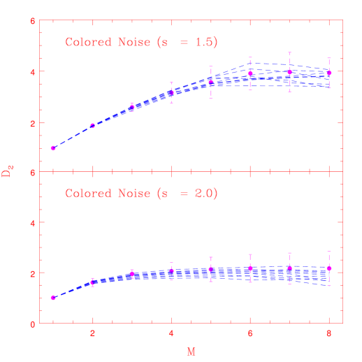
We first apply the $D_{2}$ analysis on different types of data sets such as, standard chaotic time series, pure noise and chaotic data added with noise. The time series from the standard Rossler attractor, with parameter values $a=b=0.2$ and $c=7.8$, is used as a reference to test all the computational schemes presented in this work. All computations are done with $10000$ long data points and $20$ surrogates for each data. In Fig.1, $D_{2}$ of Rossler attractor and surrogates are computed as a function of the embedding dimension $M$, where as in Fig.2, the same is shown for two pure colored noise data sets with spectral index $s=1.5$ and $2.0$. As expected, the Rossler data show clear deviation from the surrogates while for the latter, the null hypothesis cannot be rejected.

Figure 4: The $K_{2}$ values of the Rossler attractor as a function of $M$ computed using our scheme. The values are computed per sec and converges very close to the standard value $1.04\pm 0.08$.

Figure 5: Variation of $K_{2}$ with $M$ for data sets obtained by adding different amounts of white and colored noise to Rossler attractor data. The upper panel shows the result of addition of $(a)50\%$ and $(b)100\%$ white noise, while the lower panel shows the results with $(a)50\%$ and $(b)100\%$ colored noise with $s=2.0$. It is clear that while $K_{2}$ increases with addition of white noise, $K_{2}\rightarrow 0$ as the percentage of colored noise increases.

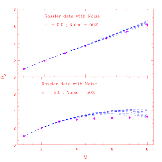
Now the real world data is often contaminated with noise and the question that arises naturally is how much amount of noise can suppress the nonlinear component that may be present in the time series. In order to study the effect of noise on $D_{2}$ using our scheme, we generate two data sets by adding $50\%$ of white and coloured noise (with $s=2.0$) to the time series from the Rossler attractor. The result of applying our scheme on these data and their surrogates is shown in Fig.3. It is found that when white noise is added to the system, $D_{2}$ of the data increases and for a contamination level of $>20\%$, it is difficult to distinguish between the data and the surrogates. But for colored noise contamination, the data is distinguishable from the surrogates for an added noise level of upto $50\%$. Note that $50\%$ noise here means that the noise amplitude is half of that of data. The above results indicate that from a $D_{2}$ analysis, it is difficult to distinguish even moderate amount of noise contamination in a chaotic data. A better quantitative measure in such a situation is $K_{2}$ discussed in the next section.

In order to get a quantification of the differences in the discriminating measure between the data and the surrogates, we use the normalised mean sigma deviation (nmsd), proposed by us recently (Harikrishnan et al., 2006). For $D_{2}$, this is computed using the expression

$$nmsd^{2}=\frac{1}{M_{max}-1}\sum_{M=2}^{M_{max}}\Big{(}\frac{D_{2}(M)-<D_{2}^{surr}(M)>}{\sigma^{surr}_{SD}(M)}\Big{)}^{2}$$ (5)

where $M_{max}$ is the maximum embedding dimension for which the analysis is undertaken, $<D_{2}^{surr}(M)>$ is the average of $D_{2}^{surr}(M)$ and $\sigma^{surr}_{SD}(M)$ is the standard deviation of $D_{2}^{surr}(M)$. We have earlier shown that a value of nmsd $<3.0$ implies either white or colored noise domination in the data and the null hypothesis cannot be rejected (see for e.g. Harikrishnan et al., 2006). It is found that for the Rossler attractor data shown in Fig.1, the nmsd = 36.1 and for the two pure colored noise in Fig.2, the nmsd = 0.68 and 2.0 for s = 1.5 and 2.0 respectively. For data contaminated by noise in Fig.3, the values are 1.8 for white noise and 3.5 for colored noise.

Figure 6: The SVD plot of the pure Rossler attractor (upper panel) along with a plot of the attractor obtained by adding $50\%$ colored noise $(s=2.0)$ to the Rossler attractor time series.

2.2 Correlation entropy

The use of $K_{2}$ has been limited compared to $D_{2}$ for the analysis of time series data. But in cases where time series involve colored noise, $K_{2}$ is a more effective discriminating measure compared to $D_{2}$ (Redaelli et al., 2002). While $D_{2}$ is a geometric measure of the underlying chaotic attractor, $K_{2}$ is a dynamic measure representing the rate at which information needs to be created as the chaotic attractor evolves in time (Ott, 1993). The standard method for the computation of $K_{2}$ is also the delay embedding technique. Since $K_{2}$ measures the rate at which the trajectory segments are increased as $M$ increases, it can be related to the correlation sum $C_{M}(R)$ by the expression

$$C_{M}(R)\propto e^{-MK_{2}\Delta t}$$ (6)

where $\Delta t$ is the time step between successive values in the time series. From above, a formal expression for $K_{2}$ can be written as,

$$K_{2}\Delta t=\lim_{R\rightarrow 0}\lim_{M\rightarrow\infty}\lim_{N\rightarrow\infty}(-{log}C_{M}(R)/M)$$ (7)

Alternately, $K_{2}$ can also be obtained as,

$$K_{2}\Delta t\equiv\lim_{R\rightarrow 0}\lim_{M\rightarrow\infty}\lim_{N\rightarrow\infty}{log}(C_{M}(R)/C_{M+1}(R))$$ (8)

Our nonsubjective scheme has been extended for the computation of $K_{2}$ as well (Harikrishnan et al., 2009a) and we apply that scheme in this work.

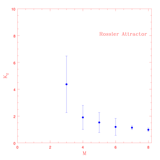
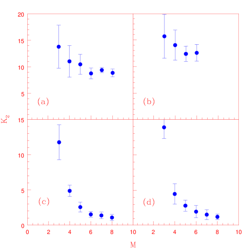
Fig.4 shows $K_{2}$ for the Rossler attractor as a function of $M$ computed from the time series using our scheme. To show the effect of noise on $K_{2}$, we generate four different time series by adding $50\%$ and $100\%$ white as well as colored noise to the Rossler attractor data. The result of applying our scheme to these data sets is shown in Fig.5. It is clear that while the saturated $K_{2}$ value increases with the white noise addition, the effect of colored noise is quite the opposite. With the increase in colored noise, the saturated value of $K_{2}\rightarrow 0$.

Figure 7: The upper panel shows the $D_{q}$ spectrum of the Rossler attractor with error bar, computed from the time series of $10000$ data points. To show the accuracy of fitting, the $D_{q}$ values (points) are again shown in the lower panel without error bar along with the best fit curve (continuous line) computed using our numerical scheme.

Figure 8: The $f(\alpha)$ spectrum of the Rossler attractor computed from the best fit $D_{q}$ curve shown in the previous figure.

Our scheme can be used for surrogate analysis with $K_{2}$ as the discriminating measure as well and nmsd can be computed using a similar expression as Eq. 5. We have applied this recently (Harikrishnan et al., 2009a) to the Rossler attractor data with different percentages of white and colored noise added. For $50\%$ white noise contamination, nmsd with $K_{2}$ as the discriminating measure is found to be $4.3$, while for the same percentage of colored noise, the value is $2.2$. Thus, while the white noise contamination can be easily identified through $D_{2}$ analysis, the presence of colored noise can be better inferred by computing $K_{2}$.

2.3 Singular value decomposition

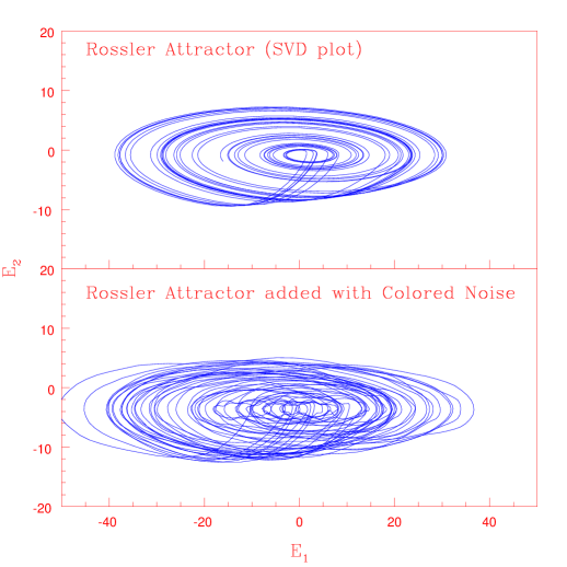
The singular value decomposition (SVD) is another important technique used in nonlinear time series analysis, first proposed by Broomhead & King (1986) and for a recent review, see Athanasiu & Pavlos (2001). The method makes use of a trajectory matrix constructed from the experimental time series with the rows of the matrix constituting the state vectors in the embedding space. It is then diagonalised to find the dominant eigen values and eigen vectors which are used to represented the dynamics. The number of dominant eigen values determine the minimum number of dimensions required to unfold the complete dynamics and the corresponding eigen vectors give the projections of the reconstructed attractors. With such a SVD projection (also called BK projection), one can visualise the qualitative nature of the reconstructed attractors. Here we use the standard TISEAN algorithm (Hegger et al., 1999) for the computation of BK projections.

Figure 9: Light curves from the twelve temporal states of the black hole system GRS1915+105. Only a part of the generated light curve is shown for clarity.

For example, the SVD projection for the Rossler attractor is shown in Fig.6 (upper panel). To show the effect of colored noise, on the SVD projection, we also show in Fig.6 (lower panel) the BK projection for the Rossler attractor added with $50\%$ colored noise with spectral index $s=2.0$. It is evident that even such large amount of colored noise does not destroy the attractor completely.

Figure 10: The power spectrum for the X-ray light curves from GRS 1915+105 in four representative states.

2.4 Multifractal spectrum

The interest of the multifractal formalism in connection with dynamical systems rests on the fact that it provides us with a very efficient method to determine the existence of strange attractors and allows a statistical description of these sets. A strange or chaotic attractor normally possess a multifractal structure as a result of the stretching and folding of the trajectories in different directions in phase space. Hence they can be characterised by a spectrum of dimensions $D(q)$ (Hentschel & Procaccia, 1983), where the index $q$ can vary from $-\infty$ to $+\infty$. The clustered regions of the attractor are characterised by $D(q)$ values with $q>0$ and rarefied regions by $D(q)$ with $q<0$, with $D(0)$ giving the simple fractal dimension of the set.

A more convenient method to represent the global scaling properties of the attractor is by using a spectrum of singularities characterising the probability measure on the strange attractor. For this, one considers the number $N_{\alpha}(\epsilon)$ of boxes (with edge length $\epsilon$) required to cover the attractor within a small range of $\alpha$ given by $\alpha\in[\alpha,\alpha+d\alpha]$. The parameter $\alpha$ is a continuous variable characterising the local scaling properties of the fractal set. Its meaning is that of a local scaling exponent:

$$\alpha_{i}=\lim_{\epsilon\rightarrow 0}{log}p_{i}(\epsilon)/{log}\epsilon$$ (9)

with $p_{i}(\epsilon)$ representing the probability measure. Thus $\alpha$ measures how fast the number of points within a box decreases as $\epsilon$ is reduced. It therefore measures the strength of a singularity for $\epsilon\rightarrow 0$. Assuming that a scaling hypothesis holds, one can write

$$N_{\alpha}(\epsilon)\propto\epsilon^{-f(\alpha)}$$ (10)

where the exponent $f(\alpha)$ represents the fractal dimension of subsets of strength $\alpha$. The graph of $f(\alpha)$ as a function of $\alpha$ is called the $f(\alpha)$ spectrum which characterises the global scaling properties of the fractal set as a function of the local scaling exponents $\alpha$. The transformation from $D(q)$ to $f(\alpha)$ can be shown to be a Legendre transformation, for details, see Halsey et al. (1986) and Atmanspacher et al. (1989b).

Figure 11: Surrogate analysis with $D_{2}$ as a discriminating measure for the light curves from four states of GRS1915+105. Note that only the $\gamma$ state is consistent with noise.

Figure 12: Same as the previous figure, but with four other states. Again, only one state - $\phi$ - shows random behavoir.

To compute the $f(\alpha)$ spectrum from a time series, we first consider the generalised correlation sum given by

$$C_{M}^{q}(R)=[{1\over N_{c}}\sum_{i}^{N_{c}}({1\over N_{v}}\sum_{j=1,j\neq i}^{N_{v}}H(R-|\vec{x_{i}}-\vec{x_{j}}|))^{q-1}]^{1/(q-1)}$$ (11)

where the Heaviside function $H$ counts how many pairs of points at $(\vec{x_{i}},\vec{x_{j}})$ are situated within a distance $R$. The spectrum of dimensions are then determined by the relation

$$D(q)\equiv\lim_{R\rightarrow 0}d({log}C_{M}^{q}(R))/d({log}(R))$$ (12)

The average value of $D_{q}$ with error bar is then calculated from the scaling region by taking different values of $R$, by extending the numerical procedure discussed above for computing $D_{2}$.

In order to determine the $f(\alpha)$ spectrum, we make use of the computational scheme recently proposed by us and applied to several practical time series (Harikrishnan et al., 2009b). The scheme uses an analytical fit for the $f(\alpha)$ function (involving a set of independant parameters) and calculates the corresponding $D_{q}$ curve using the Legendre transformation equations. This curve is then fitted to the spectrum of $D_{q}$ values computed from the time series. The best fit curve is found by changing the parameters of the $f(\alpha)$ fit, which is then used to compute the final $f(\alpha)$ spectrum. The algorithmic details of the scheme are presented elsewhere (Harikrishnan et al., 2009b). The multifractal approach has recently been employed in the analysis of several practical time series, an example being the temporal variations of the geomagnetic field (Hongre et al., 1999).

Figure 13: Variation of $K_{2}$ as a function of $M$ for the light curves from six different states of GRS1915+105. While the $K_{2}$ values of four states converge much like a low dimensional chaotic system, $K_{2}$ for the $\kappa$ state continue to decrease as $M$ increases indicating colored noise contamination. Though $K_{2}$ for $\gamma$ state converge, its value is much higher and close to that of the white noise.

Figure 14: Surrogate analysis of the light curves from four states of the black hole system with $K_{2}$ as the discriminating measure. Note that while data and the surrogates can be distinguished for $\beta$ and $\theta$, $\kappa$ and $\gamma$ behaves much like colored noise and white noise respectively.

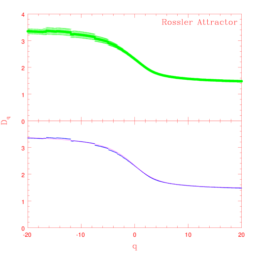
To illustrate our scheme, it is first used to compute the $f(\alpha)$ spectrum of the Rossler attractor. The spectrum of generalised dimensions $D_{q}$ is computed from the time series taking the embedding dimension $M=3$. Attempting to compute the $f(\alpha)$ spectrum directly from the $D_{q}$ values leads to an incomplete $f(\alpha)$ spectrum. This is mainly due to the fact that the errors in the calculation of $D_{q}$ makes the Legendre transformation numerically impractical because of the reversal of slopes. Hence our scheme uses a different procedure. The $f(\alpha)$ function is a single valued function defined between the limits of $\alpha_{min}$ and $\alpha_{max}$. Since the derivative $f^{\prime}(\alpha)=df(\alpha)/d\alpha=q$ is also single valued, it follows that $f(\alpha)$ has a single extremum (i.e. a maximum). Moreover, $f(\alpha_{min})=f(\alpha_{max})=0$ and $f^{\prime}(\alpha_{min})$ and $f^{\prime}(\alpha_{max})$ tend to $\infty$ and $-\infty$ respectively. A simple function which can satisfy all the above necessary conditions is,

$$f(\alpha)=A(\alpha-\alpha_{min})^{\gamma_{1}}(\alpha_{max}-\alpha)^{\gamma_{2}}$$ (13)

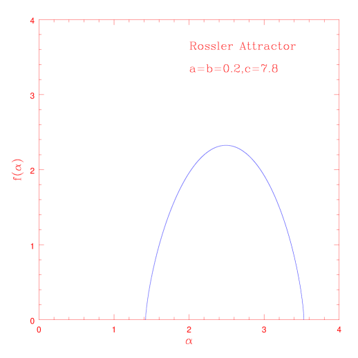
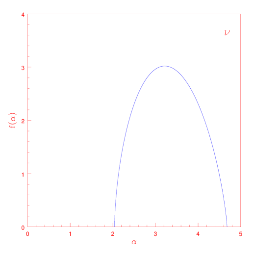
where $A$, $\gamma_{1}$, $\gamma_{2}$, $\alpha_{min}$ and $\alpha_{max}$ are a set of parameters characterising a particular $f(\alpha)$ curve. The $D_{q}$ curve can be computed from this $f(\alpha)$ fit using the inverse Legendre transformation equations for a given set of parameters. It is then fitted to the $D_{q}$ spectrum computed from the time series. The statistically best fit $D_{q}$ curve is found by adjusting the parameters of the $f(\alpha)$ function, which is then used to compute the final $f(\alpha)$ spectrum. The $D_{q}$ spectrum and its best fit curve for the Rossler attractor are shown in Fig.7 and the $f(\alpha)$ spectrum computed from the best fit curve is shown in Fig.8. Having discussed the various measures and schemes for computing them, we now turn to the analysis of the black hole system GRS1915+105.

Figure 15: The plot of the attractors underlying four states of the black hole system reconstructed via SVD analysis. Except the $\phi$ state, which behaves similar to a white noise, all the others indicate the presence of underlying attractors, the most interesting being the $\rho$ state.

3 Analysis of the Black Hole System GRS1915+105

In this section, we apply all the techniques discussed above to analyse the X-ray light curves from the black hole binary GRS1915+105. The temporal properties of the system have been classified into 12 different spectroscopic classes by Belloni et al. (2000) based on the RXTE data. Here we have chosen representative data sets for each class. The light-curve for an observation was obtained from the standard products which provide a 0.125 secs time resolution summed over all energy channels. Standard product light curves have been generated using a pipeline which considers standard filtering criteria and use data from the instruments that were reliably on. While standard products may not have optimal spectral response matrix or background model, they are more than adequate for light curve analysis, especially for bright sources, like GRS 1915+105, where the background is not important.

The analysis requires continuous data without gaps. For each class, we have extracted two sets of continuous segments for the analysis. The light curves have been generated after rebinning to a time resolution of 0.5 secs resulting in $\sim 5200$ to $6400$ continuous data points for each segment. Light curves with finer time resolutions are more Poisson noise dominated, while larger binning gives less data points. Table 1 gives the observation ID, class, number of data points etc. of all the light curves used for the analysis. In the last column, we also provide the temporal behavior of the light curve as resulted from our analysis. More details regarding the data, such as, average count, expected Poisson noise variation, etc. are given elsewhere (Misra et al., 2004).

Table 1: Details of the light curves from GRS 1915+105, in all the 12 spectral classes, used for the analysis. For each class, light curves from two Observation IDs have been analysed, as indicated. The second column gives the number of continuous data points after rebinning. The last column indicates the temporal behavior of the class as obtained from our analysis.

Obs. ID	No. of Data Points	Class	Temporal Bahavior
10408-01-10-00	6146
20402-01-46-00	5504	$\beta$	Deterministic Nonlinear
20402-01-45-00	6156
10408-01-15-00	5764	$\theta$	Deterministic Nonlinear
20402-01-03-00	6244
20402-01-31-00	5876	$\rho$	Deterministic Nonlinear
10408-01-40-00	6024
10408-01-41-00	5312	$\nu$	Deterministic Nonlinear
20187-02-01-00	6010
20402-01-22-00	5220	$\alpha$	Deterministic Nonlinear
20402-01-33-00	6240
20402-01-35-00	6244	$\kappa$	Deterministic Nonlinear + Colored Noise
20402-01-37-00	6080
20402-01-36-00	5648	$\lambda$	Deterministic Nonlinear + Colored Noise
10408-01-08-00	5688
10408-01-34-00	5756	$\mu$	Deterministic Nonlinear + Colored Noise
10408-01-17-00	6010
20402-01-41-00	5466	$\delta$	White Noise
20402-01-56-00	6324
20402-01-39-00	6180	$\gamma$	White Noise
10408-01-12-00	6286
10408-01-09-00	5580	$\phi$	White Noise
10408-01-22-00	6022
20402-01-04-00	5382	$\chi$	White Noise

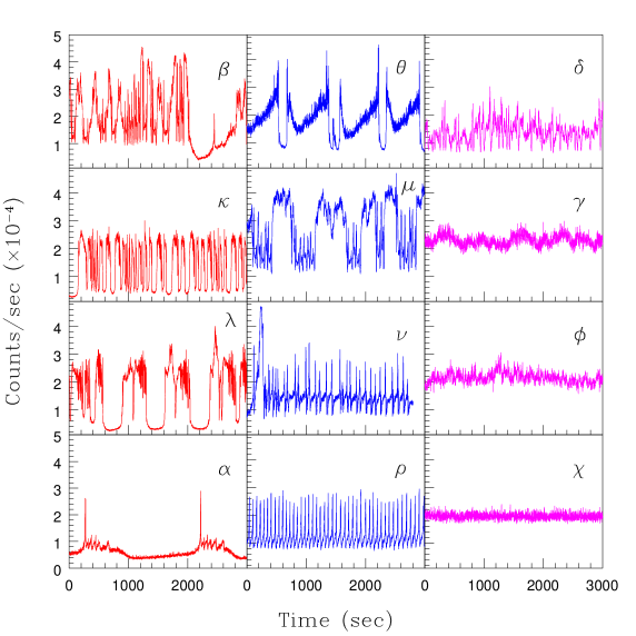
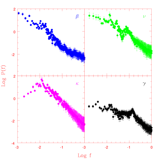
Fig.9 shows all the 12 light curves used for the analysis, which are labelled by 12 different symbols representing the 12 temporal states of the black hole system. We show only one set of light curve since the second set looks identical for all the states. The system appears to flip from one state to another randomly in time. The classification of Belloni et al. (2000) is based on a detailed analysis of all the light curves from RXTE data using various linear tools. But it is difficult to differentiate the subtle temporal features between the light curves with the help of the linear tools, such as, the power spectrum. For example, in Fig.10, we show the power spectrum for four representative states, whose temporal properties are different as per our analysis (see Table 1). While $\beta$ and $\nu$ are candidates for deterministic nonlinear behavior, $\kappa$ is possibly a mixture of nonlinearity and colored noise and $\gamma$ is purely stochastic. But these distinctions are barely evident from the power spectral variations, though the $\gamma$ state appears more like a white noise, in agreement with our results. This, once again, emphasizes the importance of methods based on nonlinear time series analysis for a better understanding of the temporal properties of the light curves.

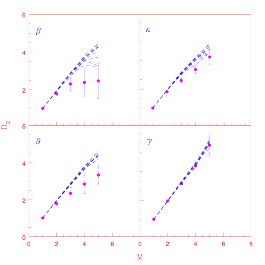
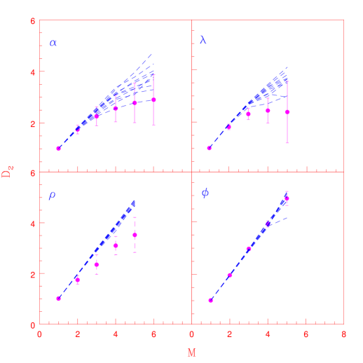
Recently, we applied surrogate analysis on all these light curves and showed that more than half of these 12 states deviated from a purely stochastic behavior (Misra et al., 2006). Here we combine the results of computations of $D_{2}$, $K_{2}$ and SVD analysis to get a better understanding regarding the nature of these light curves. We have done the surrogate analysis with $D_{2}$ and $K_{2}$ and the SVD analysis separately for the two sets of light curves. But here we only show plots from representative light curves from one set as the plots from the second set are similar and the results are qualitatively the same. Figs.11 and 12 show the results of surrogate analysis, with $D_{2}$ as discriminating measure, on eight different states. Of the states shown in these figures, it clear that only two states - $\gamma$ and $\phi$ - show purely stochastic behavior.

Figure 16: The spectrum of generalised dimensions with error bar (upper panel) for the $\nu$ state corresponding to embedding dimension $M=3$. The lower panel shows the $D_{q}$ values without error bar and the best fit curve.

Figure 17: The multifractal spectrum for the $\nu$ state computed from the best fit curve for $D_{q}$ shown in the previous figure.

Table 2: The values of nmsd computed for all the 12 GRS states from the two sets of light curves with $D_{2}$ and $K_{2}$ as discriminating measures.

GRS state	$nmsd(D_{2})$	$nmsd(D_{2})$	$nmsd(K_{2})$	$nmsd(K_{2})$
	set 1	set 2	set 1	set 2
$\beta$	7.04	9.32	13.74	11.44
$\theta$	10.63	8.59	11.20	10.86
$\alpha$	8.18	6.71	8.92	6.89
$\nu$	5.94	6.04	6.87	6.35
$\rho$	11.25	10.83	14.28	12.08
$\kappa$	4.64	4.77	3.22	3.54
$\lambda$	6.66	6.22	4.57	4.67
$\mu$	4.86	4.90	3.98	3.82
$\delta$	2.32	3.13	1.34	1.68
$\gamma$	0.88	1.03	1.83	1.43
$\phi$	0.96	0.92	2.12	1.74
$\chi$	0.78	0.73	1.67	1.38

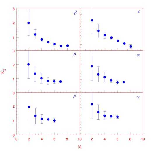
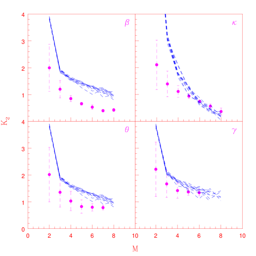
Fig.13 presents the results of computation of $K_{2}$ for six of the above eight states. Since colored noise is also expected in the black hole data, surrogate analysis has been performed with $K_{2}$ as the discriminating measure on all the 12 states. The results are shown in Fig.14 for four of these states. While the behavior of $\beta$, $\theta$ and $\gamma$ are consistent with earlier analysis, the behavior of $\kappa$ suggests that it is contaminated by colored noise.

To get a quantitative measure, we now compute nmsd using both $D_{2}$ and $K_{2}$ as discriminating measures for all the 12 states from the two sets of light curves and the results are shown in Table 2. A careful inspection of the Table reveals the following results. The values of nmsd in the two cases suggest that the temporal properties of the light curves in the two sets are almost identical. Out of the 12 states, four $(\delta,\gamma,\phi,\chi)$ are completely stochastic or white noise. Of the remaining eight states, three - $\kappa,\lambda$ and $\mu$ - are contaminated by colored noise and the rest - $\beta,\theta,\alpha,\nu$ and $\rho$ - show signatures of deterministic nonlinear behavior in their temporal variations. It is generally expected that all the states contain some amount of white noise whose percentage may vary. For example, in the case of the state $\alpha$, the saturated values of $D_{2}$ and $K_{2}$ improves significantly as the resolution time is increased from 0.5 sec to 1 sec. This clearly indicates the presence of Poisson white noise in the data. But the surrogate analysis with both $D_{2}$ and $K_{2}$ confirms that the null hypothesis can be rejected for the light curve in the $\alpha$ state.

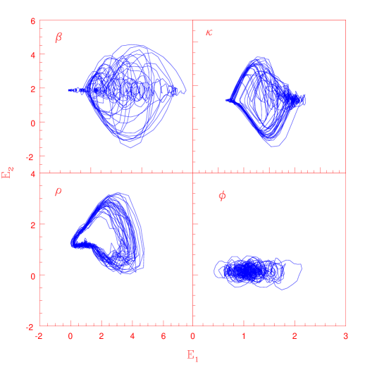
We next perform a SVD analysis on all the states which clearly show the qualitative nature of the underlying attractors. The plot of attractors for selected states are shown in Fig.15. The most interesting plot is for the $\rho$ state which shows a typical limit cycle type attractor. Also, note that the SVD plot for $\kappa$ has a nontrivial appearance, even though surrogate analysis suggested the presence of colored noise. This is also true in the case of the other two identical states, $\lambda$ and $\mu$. Thus these three states could be a mixture of deterministic nonlinearity and colored noise. Thus, based on our results, the 12 states can be divided into 3 broader classes from the point of view of their temporal properties. It turns out that some of these states which are spectroscopically different, behave identically in their nonlinear dynamics characteristics. This may be an indication of some common features in the mechanism of production of light curves from these states. The temporal behavior of each state as obtained from our analysis is indicated in the last column in Table 1. Since the behavior is identical for two different observation IDs in all cases, it may be concluded that the results presented here are not dependent on sample selection and are applicable for all the light curves classified by Belloni et al. (2000).

Figure 18: The $f(\alpha)$ spectrum for the light curves corresponding to four states of the black hole system computed using our scheme with $M=3$. Note that GRS state has been labelled alpha in order to avoid confusion with the scaling index $\alpha$.

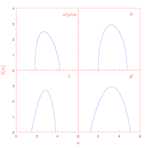
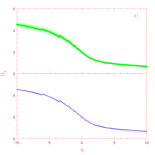
Finally, we show the results of multifractal analysis of all the light curves except the four which show purely stochastic behavior and hence the $f(\alpha)$ spectrum is irrelevant. Our non subjective scheme for computing $D_{q}$ and $f(\alpha)$ spectrum discussed in Sec. 2.4, provides us with a set of parameters that can be used to compare the fractal properties between different states as reflected in the light curves. To show the details of the computations, we first take a typical state. In Fig.16, we show the $D_{q}$ spectrum for the $\nu$ state along with the best fit curve from which the $f(\alpha)$ is computed as given in Fig.17. This is repeated for the other states as well and the results for four other states are shown in Fig.18. The multifractal nature of the attractors is evident from the figures. Since the computation is done under fixed conditions prescribed by the algorithmic scheme, the associated parameters characterising the spectra can give a better representation for comparison between various states. Our results indicate that the spectra and the associated parameters are typically different for each state and do not show any clear trend among members that display strong deterministic nonlinear behavior. This can be inferred from Fig.18 for the case of range of scales. Thus, it turns out that there are subtle differences between the states belonging to the same dynamic class with respect to multifractal scaling as well, apart from linear spectral characteristics based on which the 12 states are divided.

4 Discussion and Conclusion

Identifying nontrivial structures in real world systems is considered to be a challenging task as it requires a succession of tests using various quantitative measures. Eventhough a large number of potential systems from various fields have been analysed so far, the results remain inconclusive in many cases. Here we present an example of a very interesting astrophysical system, which we analyse using several important quantifiers of low dimensional chaos. By using the time series from a standard chaotic system - the Rossler attractor - we first test the computational schemes used for the analysis. These schemes are then applied to the light curves from the black hole system. We find that out of the 12 spectroscopic states, only four are purely stochastic. The remaining show signatures of deterministic nonlinearity, with three of them contaminated by colored noise. All these 8 states are found to have $D_{2}<4$ so that their complex temporal behavior can be approximated by 3 or 4 coupled ordinary differential equations. Based on our results, the 12 states can be broadly classified into three from a dynamical perspective: purely stochastic with $D_{2}\rightarrow\infty$, affected by colored noise and those which are potential candidates for low dimensional $(D_{2}<4)$ chaotic behavior.

It should be noted that Belloni et al. (2000) classified the light curves into 12 states based on their count rate, variability and spectral characteristics. In other words, this is a classification based on linear characteristics of the light curves. Ours is not a classification as in the strict sense of Belloni et al. (2000). We only show that some of the light curves which appear different based on their variability and spectral properties can be grouped together when viewed from a dynamical perspective.

Our results could be significant in many ways. First of all, this is the first real evidence of a possible multifractal attractor in the time series of a black hole system. The fact that the light curves from many of the temporal states have underlying strange attractor like behavior, increases the possibility that the temporal variability in the time scales within these states are governed by some inherent nonlinear processes with a few degrees of freedom. In other words, the complex nonlinear partial differential equations that are known to govern the hydrodynamic flow can be approximated by a set of ordinary differential equations and hence can be more easily studied and understood. Moreover, the result that some of the states which are spectroscopically different, have approximately the same nonlinear characteristics is interesting from certain dynamical aspects, such as the mechanism of production of light curves. It is well known that GRS1915+105 is a unique black hole system with many temporal states which vary over a wide range of time scales. Many of the questions regarding this variability and the exact mechanism of production of light curves still remain unanswered.

Another question is regarding the structure of variability between the 12 spectroscopic states. It has been suggested that all the observed light curves could be interpreted in terms of three basic states (a hard state and two softer states) and a sequence of transitions between them (Belloni et al., 2000). This could, in principle, give rise to a much larger variety of light curves. But the system chooses only a handful of these sequences. This possibly suggests that the structure of time variability is not random, but controlled by some physical parameter which must be connected to the basic properties of the accretion disk. The presence of deterministic nonlinear behavior in the system further substantiates this idea.

Interestingly, the system appears to be in the $\chi$ state for most of the time which is identified as purely stochastic in our analysis. We have also analysed many samples of the long time average of the light curves from the system and found that they show purely random bahavior. Thus, one possibility is that the states other than the $\chi$ state may well be short time flips due to some changes taking place within the system. But many of these short time states pick up much less amount of noise revealing, for example, the underlying nonlinear character. Thus, an interesting question is whether the states such as $\beta$ and $\theta$ have a different underlying mechanism of production of light curves compared to the $\chi$ state. Or, is the excessive amount of white noise in that state itself is suppressing the nonlinear properties? The question whether the different states are temporal manifestations of a single underlying mechanism or are they dynamically different, will be vital for a proper modelling of this fascinating astrophysical object.