CLP-based protein fragment assembly

Abstract

The paper investigates a novel approach, based on Constraint Logic Programming (CLP), to predict the 3D conformation of a protein via fragments assembly. The fragments are extracted by a preprocessor—also developed for this work— from a database of known protein structures that clusters and classifies the fragments according to similarity and frequency. The problem of assembling fragments into a complete conformation is mapped to a constraint solving problem and solved using CLP. The constraint-based model uses a medium discretization degree $C\alpha$-side chain centroid protein model that offers efficiency and a good approximation for space filling. The approach adapts existing energy models to the protein representation used and applies a large neighboring search strategy. The results shows the feasibility and efficiency of the method. The declarative nature of the solution allows to include future extensions, e.g. different size fragments for better accuracy.

Note: This article has been published in Theory and Practice of Logic Programming, 10 (4-6): 709 -724, July ©Cambridge University Press.

1 Introduction

Proteins are central components in the way they control and execute the vital functions in living organisms. The functions of a protein are directly related to its peculiar three-dimensional conformation. Knowledge of the three-dimensional conformation of a protein (also known as the native conformation or tertiary structure) is essential to biomedical investigation. The native conformation represents the functional protein and determines how it can interact with other proteins and affect the functions of the hosting organism. It is impossible to clearly understand the behavior and phenotype of an organism without knowledge of the native conformation of the proteins coded in its genome. As a result of advancements in DNA sequencing techniques, there is a large and growing number of protein sequences—i.e., lists of amino acids, also known as primary structures of proteins—available in public databases (e.g., the database Swiss-prot contains about $500,000$ protein sequences). On the other hand, knowledge of structural information (e.g., information concerning the tertiary structures) is lagging behind, with a much smaller number of structures deposited in public databases, notwithstanding that structural genomics initiatives started worldwide.

For these reasons, one of the most traditional and central problems addressed by research in bioinformatics deals with the protein structure prediction problem, i.e., the problem of using computational methods to determine the native conformation of a protein starting from its primary sequence. Several approaches have been explored to address this problem. In broad terms, it is possible to distinguish between two main classes of approaches. The more traditional term protein structure prediction has been commonly used to describe methods that rely on comparisons between known and unknown proteins to predict the end-result of the spontaneous protein folding process (also known as homology modeling). The more expensive task of predicting a protein structure starting from the knowledge of the chemical structure and laws of physics (known as de-novo/ab-initio prediction) has been studied with different levels of accuracy and complexity.

Instead, protein folding simulations tries to understand the folding path leading to the native conformation, typically using investigations of the potential energy landscape or using molecular dynamics simulations. In both classes of methods, knowledge of “patterns” can be used to restrict the search space—and this is particularly true for the case of secondary structure components of a protein, i.e., local helices or strands. Secondary structure components are important, considering that their formation is believed to represent the earliest phase of the folding process, and their identification can be relatively simpler (e.g., through low-resolution observations of images from electron microscopy).

1.1 Related work

As mentioned above, it is possible to predict protein structures based on their sequences, using either homology modeling or fold recognition techniques. Nevertheless, it is in general difficult to predict a protein structure based only on its sequence and in absence of structural templates. Explicit solvent molecular dynamics simulations of protein folding are still beyond current computational capabilities. Already in 1968, Levinthal postulated that the systematic exploration of the space of possible conformations is infeasible [Levinthal (1968)]. This complexity has been confirmed by theoretical results, showing that even extremely simplified formalizations of the problem lead to computationally intractable problems [Crescenzi et al. (1998)]. Recently, ab-initio methods for generating protein structures given their sequences have been proposed and successfully used [Ben-David et al. (2009)]. Key elements of these methods are the use of evolutionary information from multiple alignments, the adoption of simplified representations of proteins, and the introduction of fragments assembly techniques. These methods rely on assembling the structure using simplified representations of protein fragments with favorable conformations (obtained from structural databases) for the profile of the given sequence. Three to nineteen-residue fragments (i.e., 3–9 for small proteins and 5–19 for large ones) contain correlations among neighboring residue conformations, and most of the computation time is spent in finding the global arrangement of fragments that already display good local conformations [Raman et al. (2009), Wu et al. (2007)].

Several simplified models have been introduced to address the problem. Simplified models abstract several properties of both proteins and space, leading to a version of the problem that can be solved more efficiently. The solutions of the simplified problem constitute candidate configurations that can be refined with more computationally intensive methods, e.g., molecular dynamics simulations. Possible simplifications include the introduction of fixed sizes of monomers and bond lengths, the representation of monomers as simple points, and viewing the three-dimensional space as a discretized collection of points. In these simplified models, it is possible to view the protein folding problem as an optimization problem, aimed at determining conformations that minimize an energy function. The energy function must be defined according to the simplified model adopted [Berrera et al. (2003), Fogolari et al. (2007)]. Simplified energy models have been devised specifically to solve large instances of the structure prediction problem using constraint solving approaches [Backofen and Will (2006), Dotu et al. (2008)].

In our own previous efforts, we have applied declarative programming approaches, based on constraint solving, to address the problem. We built our efforts on a discrete crystal lattice organization of the allowable points in the three-dimensional space. This representation exploits the property that the distance between the $C\alpha$ atoms of two consecutive amino acids is relatively constant (3.8Å). The problem is viewed as placing amino acids in the allowable points, in such a way that constraints encoding the mutual distances of amino acids in the primary sequence are satisfied [Dal Palù et al. (2004), Dal Palù et al. (2007)]. The original framework has also been expanded to support several types of global constraints, i.e., constraints describing complex relationships among groups of amino acids. One of these constraints is the rigid structure constraint—this constraint enables the representation of known substructures (e.g., secondary structure components), reducing the problem to the determination of an appropriate placement and rotation of such substructures in the lattice space. The ability to use rigid structure constraints has been shown to lead to dramatic reductions in the search space [Dal Palù et al. (2010), Barahona and Krippahl (2008)]. However, exploiting knowledge of real rigid substructures in a discrete lattice is infeasible, due to the errors introduced by the approximations imposed by the discretized representation of the search space. On the other hand, the use of a less constrained space model leads to search spaces that are intractable. These two considerations lead to the new approach presented in this work.

1.2 The contribution of this work

Some of the most successful approaches to protein folding build on the principles of using substructures. The intuition is that, while the complete folding of a protein may be unknown, it is likely that all possible substructures, if properly chosen, can be found among proteins whose conformations are known. The folding can be constructed by exploiting relationships among substructures. A notable example of this approach is represented by Rosetta [Raman et al. (2009)]—an ab initio protein structure prediction method that uses simulated annealing search to compose a conformation, by assembling substructures extracted from a fragment library; the library is obtained from observed structures stored in the Protein Data Bank (PDB, www.pdb.org).

In this work, we follow a similar idea, by developing a database of amino acid chains of length $4$; these are clustered according to similarity, and their frequencies are drawn from the investigation of a relevant section of the Protein Data Bank. The database contains the data needed to solve the protein folding problem via fragments assembly. Declarative programming techniques are used to generate clean and compact code, and to enable rapid prototyping. Moreover, the problem of assembling substructures is efficiently tackled using the constraint solving techniques provided by $CLP(\mathcal{FD})$ systems.

This paper has the goal of showing that our approach is feasible. The main advantage, w.r.t. a highly engineered and imperative tool, is the modularity of the constraint system, which offers a convenient framework to test and integrate statistical data from various predictors and databases. Moreover, the constrained search technique itself represents a novel method, compared to popular predictors, and we show its effectiveness in combination with the development of new energy functions and heuristics. The proposed solution includes a general implementation of large neighboring search in $CLP(\mathcal{FD})$, that turned out to be highly effective for the problem at hand. Another contribution is the development of a new energy function based on two components: a contact potential for backbone and side chain centroids interaction, and an energy component for backbone conformational preferences. Backbone and side chain steric hindrances are imposed as constraints.

2 Protein Abstraction

2.1 Preliminary notions

We focus on proteins described as sequences of amino acids selected from a set $\mathbb{A}$ of 20 elements (those coded by the human genome). In turn, each amino acid is composed of a set of atoms that constitute the amino acid’s backbone (see Fig. 1) and a set of atoms that differentiate pairs of amino acids, known as side chain. One of the most important structural properties is that two consecutive $C\alpha$ atoms have an average distance of 3.8Å. Side chains may contain from 1 to 18 atoms, depending on the amino acid. For computational purposes, instead of considering all atoms composing the protein, we consider a simplified model in which we are interested in the position of the $C\alpha$ atoms (representing the backbone of the protein) and of particular points, known as the centroids of the side chains (Fig. 3). A natural choice for the centroid is the center of mass of the side chain.

It is important to mention that, once the positions of all the $C\alpha$ atoms and of all the centroids are known, the structure of the protein is already sufficiently determined, i.e., the position of the remaining atoms can be identified almost deterministically with a reasonable accuracy.

ALA $\mapsto$ 0 LEU $\mapsto$ 1 MET $\mapsto$ 1 ARG $\mapsto$ 2 GLU $\mapsto$ 2 GLN $\mapsto$ 2 LYS $\mapsto$ 2 ASN $\mapsto$ 3 ASP $\mapsto$ 3 SER $\mapsto$ 3 THR $\mapsto$ 4 PHE $\mapsto$ 4 HIS $\mapsto$ 4 TYR $\mapsto$ 4 ILE $\mapsto$ 5 VAL $\mapsto$ 5 TRP $\mapsto$ 5 CYS $\mapsto$ 6 GLY $\mapsto$ 7 PRO $\mapsto$ 8

Figure 1: Two consecutive amino acids and the clustering of amino acids into 9 classes

Focusing on the backbone and on the $C\alpha$ atoms, three consecutive amino acids define a bend angle (see $\theta$ in Fig. 2—left). Consider now four consecutive amino acids $a_{1},a_{2},a_{3},a_{4}$. The angle formed by $n_{2}\mathchar 61\relax(a_{4}\mathchar 45\relax a_{3})\times(a_{3}\mathchar 45\relax a_{2})$ and $n_{1}\mathchar 61\relax(a_{3}\mathchar 45\relax a_{2})\times(a_{2}\mathchar 45\relax a_{1})$ is called torsional angle (see $\phi$ in Fig. 2—right). If these angles are known for all the consecutive 4-tuples forming a protein, they uniquely describe the 3D positions of all the $C\alpha$ atoms of the protein.

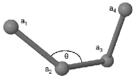
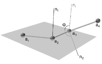
Figure 2: Bend (left) and torsional (right) angles

Given a spatial conformation of a 4-tuple of consecutive $C\alpha$ atoms, a small degree of freedom for the position of the side chain is allowed—leading to conformers commonly referred to as rotamers. To reduce the search space, we do not consider such variations. Once the positions of the $C\alpha$ atoms are known, we deterministically add the positions of the centroids. In particular, the centroid of the $i$-th residue is constructed by using the positions of $C\alpha_{i\mathchar 45\relax 1}$, $C\alpha_{i}$ and $C\alpha_{i\mathchar 43\relax 1}$ as reference and by considering the average of the center of mass of the same amino acid type centroids, sampled from a non-redundant subset of the PDB. The parameters that uniquely determine its position are: the average $C\alpha$-side chain center of mass distance, the average bend angle formed by the side chain center of mass-$C\alpha_{i}$-$C\alpha_{i\mathchar 43\relax 1}$, and the torsional angle formed by the $C\alpha_{i\mathchar 45\relax 1}$-$C\alpha_{i}$-$C\alpha_{i\mathchar 43\relax 1}$-side chain center of mass. Even with this simplification, the introduction of the centroids in the model allows us to better cope with the layout in the 3D space and to use a richer energy model. In Fig. 3, we report an example of this abstraction with a fragment with 10 alanines (ALA). For these amino acids, the centroids coincide with the only heavy atom of each sidechain.

This has been experimentally shown to produce more accurate results, without adding extra complexity w.r.t. a model that considers only the positions of the $C\alpha$ atoms and without the use of centroids.

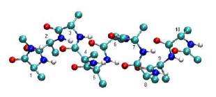
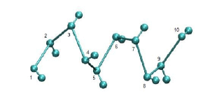
Figure 3: A fragment of 10 ALA amino acids in all-atom and $C\alpha$-centroid representation

2.2 Clustering

Although more than 60,000 protein structures are present in the PDB, the complete set of known proteins contains too much redundancy (i.e., very similar proteins deposited in several variants) to be useful for statistical purposes. Therefore we focused on a subset of the PDB called top-500 [Lovell et al. (2003)]. This set contains 500 proteins, with $107,138$ occurrences of amino acids. The number of different 4-tuples occurring in the set is precisely $62,831$. Since the number of possible 4-tuples of amino acids is $|\mathbb{A}^{4}|\mathchar 61\relax{20}^{4}\mathchar 61\relax 160,000$, this means that most 4-tuples do not appear in the selected set; even those that appear, occur too rarely to provide significant statistical information. For this reason, we decided to cluster amino acids into 9 classes, according to the similarity of the torsional angles of the pseudo bond between two consecutive $C\alpha$ atoms [Fogolari et al. (2007)]. Note that, in our simplified model, two consecutive $c_{\alpha}$ atoms do not form a covalent bond and this fact is indicated by the term pseudo.

Let $\gamma:\mathbb{A}\longrightarrow\{0,\dots,8\}$ be the function assigning a class to each amino acid, as defined in Fig. 1; for $i\in\{0,\dots,8\}$, let us denote with $\gamma^{\mathchar 45\relax 1}(i)\mathchar 61\relax\{a\in\mathbb{A}\,:\,\gamma(a)\mathchar 61\relax i\}$. In this way, the majority of the $9^{4}\mathchar 61\relax 6,561$ 4-tuples have a representative in the set (precisely, there are templates for $5,830$ of them).

A second level of approximation is introduced in deciding when two occurrences of the same 4-tuple have the “same” form. The two tuples are placed in the same class when their Root Mean Square Deviation (RMSD) is less than or equal to a given threshold (rmsd_thr); this threshold is currently set to 1.0Å. We developed a C program, called tuple_generator, that creates a set of facts of the form:

$$\begin{array}[]{ll}{\mathtt{t}uple}(&[g_{1},g_{2},g_{3},g_{4}],\phantom{aa}[X^{\alpha}_{1},Y^{\alpha}_{1},Z^{\alpha}_{1},X^{\alpha}_{2},Y^{\alpha}_{2},Z^{\alpha}_{2},X^{\alpha}_{3},Y^{\alpha}_{3},Z^{\alpha}_{3},X^{\alpha}_{4},Y^{\alpha}_{4},Z^{\alpha}_{4}],\\ &\mbox{$g_{2}$-centroid-list},\phantom{aa}\mbox{$g_{3}$-centroid-list},\phantom{aa}{\mathtt{F}REQ},\phantom{aa}{\mathtt{I}D},\phantom{aa}{\mathtt{P}ID})\end{array}$$

where $[g_{1},g_{2},g_{3},g_{4}]\in\{0,\dots,8\}^{4}$ identifies the class of each amino acid, $X^{\alpha}_{1},\dots,Z^{\alpha}_{4}$ are the coordinates of the 4 $C\alpha$ atoms of the 4-tuple, ${\mathtt{F}REQ}\in\{0,\dots,1000\}$ is a frequency factor of the template w.r.t. all occurrences of the 4-tuple $g_{1},\dots,g_{4}$ in the set top-500, $\mathtt{I}D$ is a unique identifier for this fact, and $\mathtt{P}ID$ is the first protein found containing this template; this last piece of information will be printed in the file we produce as output of the computation, in order to allow one to recover the source of a fragment used for the prediction.

As discussed in Sect. 2.1, we model the position of the centroid of the side chain of every amino acid. $g_{i}\in\{0,\dots,8\}$ is a representative of the class of amino acids $\gamma^{\mathchar 45\relax 1}(g_{i})$ (e.g., $\gamma^{\mathchar 45\relax 1}(2)\mathchar 61\relax\{\mathrm{ARG},\mathrm{GLU},\mathrm{GLN},\mathrm{LYS}\}$—see Fig. 1). For each amino acid $a\in\gamma^{\mathchar 45\relax 1}(g_{i})$, we compute the position of the centroid corresponding to the positions $X^{\alpha}_{1},\dots,Z^{\alpha}_{4}$ of the $C\alpha$ atoms, and add it to the $g_{i}$-centroid-list. Let us observe that we do not add the position of the first and last centroid in the 4-tuples. As a result, at the end of the computation, only the centroid of the first and the last amino acids of the entire protein will be not set; these can be assigned using a straightforward post-processing step.

It is unlikely that a 4-tuple $a_{1},\dots,a_{4}$ that does not appear in the considered training set will occur in a real protein. Nevertheless, in order to handle these cases, if $[\gamma(a_{1}),\dots,\gamma(a_{4})]$ has no statistics associated to it, we map it to the special 4-tuple $[\mathchar 45\relax 1,\mathchar 45\relax 1,\mathchar 45\relax 1,\mathchar 45\relax 1]$. By default, we assign to this unknown tuple the set of 6 most common templates (the number can be easily increased) among the set of all known templates. Other special 4-tuples are $[\mathchar 45\relax 2,\mathchar 45\relax 2,\mathchar 45\relax 2,\mathchar 45\relax 2]$ and $[\mathchar 45\relax 3,\mathchar 45\relax 3,\mathchar 45\relax 3,\mathchar 45\relax 3]$; these are assigned to $\alpha$-helices and $\beta$-sheets every time a secondary structure constraint is locally enforced on a region of the conformation. Handling of these special tuples will be described in detail in Section 3.1.

We also introduce an additional collection of facts, based on the predicate next, which are used to relate pairs of tuple facts. The relation ${\mathtt{n}ext}({\mathtt{I}D}_{1},{\mathtt{I}D}_{2},{\mathtt{M}at})$ holds if the last three amino acids of the sequence in the tuple fact identified by ${\mathtt{I}D}_{1}$ are identical to the first three amino acids of the sequence in the tuple fact ${\mathtt{I}D}_{2}$, and the corresponding $C\alpha$ sequences are almost identical—in the sense that the RMSD between them is at most rmsd_thr. $\mathtt{M}at$ is the rotation matrix to align the 1–3 $C\alpha$ atoms of the 4-tuple of ${\mathtt{I}D}_{2}$ with the 2–4 $C\alpha$ atoms of the 4-tuple of ${\mathtt{I}D}_{1}$.

2.3 Statistical energy

The energy function used in this work builds on two components: (1) a contact potential for side chain and backbone contacts and (2) an energy component for each backbone conformation based on backbone conformational preferences observed in the database. The first component uses the table of contact energies described in [Berrera et al. (2003)]. This set of energies has been shown to be accurate, and it is the result of filtering the dataset to allow accurate statistical analysis, and a consequent fine tuning of the contact definition. Since not all side chain atoms are represented, it is not possible to directly use the definition of [Berrera et al. (2003)]; therefore, we retain the table of contact energies of [Berrera et al. (2003)], but we adapt the contact definition to the side chain centroid. In particular, we use the value $3\mathbin{\cdot}2$Å as the shortest distance between two centroids, and we set the contact distance between two centroids to be less than or equal to the sum of their radii. Larger distances provide a contribution that decays quadratically with the distance.

The radius of each centroid is computed as the centroid’s average distance from the $C\alpha$ atom. No contact potential is assigned to the side chain’s $C\alpha$, as the side chain definition already includes the $C\alpha$ carbon. The energy assigned to the contact between backbone atoms represented by $C\alpha$ (not included in the side chain definition) is the same energy assigned to ASN-ASN contacts, which involve mainly similar chemical groups contacts. The torsional angle defined by four consecutive $C\alpha$ atoms is assigned an energy value defined by the potential of the mean force derived by the distribution of the corresponding torsional angle in the PDB. The procedure has been thoroughly described in [Fogolari et al. (2007)].

3 Modeling

In this section, we describe the modeling of the problem of fragments assembly using constraints over finite domains—specifically, the type of constraints provided in $CLP(\mathcal{FD})$. The input is a list ${\mathtt{P}rimary}$ of $n$ amino acids. We will denote with $a_{i}$ the $i^{th}$ element of the primary sequence. We also allow PDB identifiers as inputs; in this case, the primary structure of the protein is retrieved from the PDB. A list of $n\mathchar 45\relax 3$ variables (Code) is generated. The $i$-th variable $C_{i}$ of Code corresponds to the 4-tuple $(\gamma(a_{i}),\dots,\gamma(a_{i\mathchar 43\relax 1}),\gamma(a_{i\mathchar 43\relax 2}),\gamma(a_{i\mathchar 43\relax 3}))$. The possible values for $C_{i}$ are the $\mathtt{I}D$s of the facts of the form:

$${\mathtt{t}uple}([\gamma(a_{i}),\gamma(a_{i\mathchar 43\relax 1}),\gamma(a_{i\mathchar 43\relax 2}),\gamma(a_{i\mathchar 43\relax 3})],\_,\_,{\mathtt{F}req},{\mathtt{I}D},\_)\mathbin{\cdot}$$

This set is ordered using the frequency information Freq in decreasing order, and stored in a variable ${\mathtt{L}istDom}_{i}$.

The next information is used to impose constraints between $C_{i}$ and $C_{i\mathchar 43\relax 1}$. Using the combinatorial constraint table, we allow only pairs of consecutive values supported by the next predicate. Recall that, for each allowed combination of values, the next predicate returns the rotation matrix ${\mathtt{M}_{i,i\mathchar 43\relax 1}}$, which provides the relative rotation when the two fragments are best fit.

Another list with $3n$ variables (Tertiary) is also generated: $X^{\alpha}_{i},Y^{\alpha}_{i},Z^{\alpha}_{i}$ (resp., $X^{C}_{i},Y^{C}_{i},Z^{C}_{i}$) denoting the 3D position of the $C\alpha$ atoms (resp., of the centroids). These variables have integer values (representing a precision of $10^{\mathchar 45\relax 2}$Å).

In order to correlate Code variables and Tertiary variables, consecutive 4-tuples must be constrained. Let us focus on the $C\alpha$ part; consider two consecutive tuples:

• $t_{i}\mathchar 61\relax a_{i},a_{i\mathchar 43\relax 1},a_{i\mathchar 43\relax 2},a_{i\mathchar 43\relax 3}$ with code variable $C_{i}$, and

• $t_{i\mathchar 43\relax 1}\mathchar 61\relax a_{i\mathchar 43\relax 1},a_{i\mathchar 43\relax 2},a_{i\mathchar 43\relax 3},a_{i\mathchar 43\relax 4},$ with code variable $C_{i\mathchar 43\relax 1}$ and local coordinates $\vec{V}_{1},\vec{V}_{2},\vec{V}_{3},\vec{V}_{4}$.

$t_{i\mathchar 43\relax 1}$ is rotated as to best overlap the points in common with $t_{i}$, and it is placed so that the last point in $t_{i\mathchar 43\relax 1}$ is at 3.8Å from the last point in $t_{i}$.

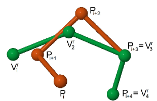
Figure 4: Consecutive fragments combination

Let $X^{\alpha}_{i},Y^{\alpha}_{i},Z^{\alpha}_{i},\dots,X^{\alpha}_{i\mathchar 43\relax 4},Y^{\alpha}_{i\mathchar 43\relax 4},Z^{\alpha}_{i\mathchar 43\relax 4}$ be the variables for the coordinates of these $C\alpha$ atoms, stored in the list Tertiary (Fig. 4, where $P_{i}\mathchar 61\relax(X^{\alpha}_{i},Y^{\alpha}_{i},Z^{\alpha}_{i})$). The constraint introduced rotates and translates the template $t_{i\mathchar 43\relax 1}$ from the reference of $C_{i}$ (represented by the orthonormal basis matrix ${\mathtt{R}_{i}}$) according to the rotation matrix ${\mathtt{M}_{i,i\mathchar 43\relax 1}}$ to the new reference ${\mathtt{R}_{i\mathchar 43\relax 1}}\mathchar 61\relax{\mathtt{R}_{i}}\times{\mathtt{M}_{i,i\mathchar 43\relax 1}}$. Moreover, when placing the template $t_{i\mathchar 43\relax 1}$, the constraint affects only the coordinates of $a_{i\mathchar 43\relax 4}$, since the other variables are assigned by the application of the same constraint for templates $t_{j}$, $j\mathchar 60\relax i\mathchar 43\relax 1$. The constraint shifts the rotated version of $t_{i\mathchar 43\relax 1}$ so that it overlaps the third point $\vec{V}_{3}$ with $(X^{\alpha}_{i\mathchar 43\relax 3},Y^{\alpha}_{i\mathchar 43\relax 3},Z^{\alpha}_{i\mathchar 43\relax 3})$. Formally, let $\vec{V}^{r}_{k}\mathchar 61\relax{\mathtt{R}_{i\mathchar 43\relax 1}\times\vec{V}_{k}}$, with $k\in\{1\dots 4\}$, be the rotated 4-tuple corresponding to $C_{i\mathchar 43\relax 1}$. The shift vector $\vec{s}\mathchar 61\relax(X^{\alpha}_{i\mathchar 43\relax 3},Y^{\alpha}_{i\mathchar 43\relax 3},Z^{\alpha}_{i\mathchar 43\relax 3})\mathchar 45\relax\vec{V}^{r}_{3}$ is used to constrain the position of $a_{i\mathchar 43\relax 4}$ as follows:

$$(X^{\alpha}_{i\mathchar 43\relax 4},Y^{\alpha}_{i\mathchar 43\relax 4},Z^{\alpha}_{i\mathchar 43\relax 4})\mathchar 61\relax\vec{s}\mathchar 43\relax{\mathtt{R}_{i\mathchar 43\relax 1}}\times\vec{V}_{4}$$

Note that the 3.8Å distance between consecutive amino acids (i.e., $a_{i\mathchar 43\relax 3}$ and $a_{i\mathchar 43\relax 4}$) is preserved, and this constraint allows us to place templates without requiring an expensive RMSD fit among overlapping fragments during the search. Moreover, during a leftmost search, as soon as the variable $C_{i}$ is assigned, also the coordinates $(X^{\alpha}_{i\mathchar 43\relax 3},Y^{\alpha}_{i\mathchar 43\relax 3},Z^{\alpha}_{i\mathchar 43\relax 3})$ are uniquely determined.

Matrix and vector products are handled by FD variables and constraints, using a factor of 1000 for storing and handling rotation matrices.

For the sake of simplicity, we omit the formal description of the constraints associated to the centroids. The centroids’ positions are rotated and shifted accordingly, as soon as the corresponding positions of the $C\alpha$ atoms are determined.

The $X_{1}^{\alpha},Y_{1}^{\alpha},Z_{1}^{\alpha},\dots,X_{n}^{\alpha},Y_{n}^{\alpha},Z_{n}^{\alpha}$ part of the Tertiary list relative to the position of the $C\alpha$ atoms, is also required to satisfy a constraint which guarantees the all_distant property [Dal Palù et al. (2010)]: the $C\alpha$ atoms of each pair of non-consecutive amino acids must be distant at least $D\mathchar 61\relax 3\mathbin{\cdot}2$Å. This is expressed by the constraint:

$$(X_{i}^{\alpha}\mathchar 45\relax X_{j}^{\alpha})^{2}\mathchar 43\relax(Y_{i}^{\alpha}\mathchar 45\relax Y_{j}^{\alpha})^{2}\mathchar 43\relax(Z_{i}^{\alpha}\mathchar 45\relax Z_{j}^{\alpha})^{2}\geq D^{2}$$

for all $i\in\{1,\dots,n\mathchar 45\relax 2\}$ and $j\in\{i\mathchar 43\relax 2,\dots,n\}$. Similar constraints are imposed between pairs of $C\alpha$ and centroids as well as pairs of centroids. In the latter case, in order to account for the differences in volume of each possible side chain, we determine minimal distances that depend on the specific type of amino acid considered.

Another constraint is added to guide the search: a diameter parameter is used to bound the maximum distance between different $C\alpha$ atoms (i.e., the diameter of the protein). As we argued in earlier work [Dal Palù et al. (2004)], a good diameter value is $5\mathbin{\cdot}68\,n^{0\mathbin{\cdot}38}$ Å. We impose this constraint to all different pairs of $C\alpha$ atoms.

3.1 Secondary information

The native structure of a protein is largely composed of some recurrent local structures. These structures, $\alpha$-helices and $\beta$-sheets, can be predicted with good accuracy using efficient techniques, such as neural networks, or recognized using other techniques (e.g., analysis of density maps from electron microscopy). Being based on frequency analysis, our tool is able to discover the majority of secondary structures. On the other hand, a-priori knowledge of these structures allows us to remove several non-deterministic choices during computation. Therefore, we allow knowledge of secondary structures to be provided as part of the input—e.g., information indicating that the amino acids $i$–$j$ form an $\alpha$-helix. In the processing stage, for $k\in\{i,\dots,j\mathchar 45\relax 3\}$, a particular tuple $[\mathchar 45\relax 2,\mathchar 45\relax 2,\mathchar 45\relax 2,\mathchar 45\relax 2]$ is assigned instead of the tuple $[\gamma(a_{k}),\dots,\gamma(a_{k\mathchar 43\relax 3})]$. This tuple has a unique template which is associated to an $\alpha$-helix, built in a standard way using a bend angle of 93.8 degrees and a torsional angle of 52.3 degrees. Moreover, a list of the possible positions for the centroids of the 20 amino acids is retrieved. Since the domains for these $C_{k}$’s are singletons, as soon as $C_{i}$ is considered for value assignment, all the points of the helix are deterministically computed. The situation in the case of $\beta$-strands is analogous.

A variation of this technique can be used if larger and more complex substructures are known. Basically, even keeping just 4-tuples as internal data structures, we can easily deal with tuples of arbitrary lengths. Automated manipulation of arbitrary complex structures is subject of future work.

4 Searching

The search is guided by the instantiation of the $C_{i}$ variables. These variables are instantiated in leftmost-first order; in turn, the values in their domains are attempted starting with the most probable value first. We observed that a first-fail strategy does not speed up the search, probably due to the weak propagation of the matrix product constraints. As described in Section 2.3, we associate an energy to each computed structure. The energy value is an FD constraint that links coordinates variables and amino acids. Given the model of the problem, this kind of constraint is not able to provide effective bounds for pruning the search space when searching for optimal solutions. As future work, we plan to investigate specific propagators, since the torsional energy contribution could be exploited for exact bounds estimations.

Each computed structure is saved in pdb format. This is a standard format for proteins (detailed in the PDB repository) that can be processed by most protein viewers (e.g., Rasmol, ViewerLite, JMol).

In order to further reduce the time to search for solutions, we have developed a logic programming implementation of Large Neighboring Search (LNS) [Shaw (1998)]. LNS is a form of local search, where the search for the successive solutions is performed by exploring a “large” neighborhood. The traditional basic move used in local search, where the values of a small number of variables are changed, is replaced by a more general move, where a large number of variables is allowed to change, and these variables are subject to constraints. The basic LNS routine is the following:

• Generate an initial solution (e.g., using the standard CLP labeling procedure).

• Randomly select a subset of the variables of the problem that are admissible for changes, and assign the previous values to the other variables.

• Using standard labeling, look for an assignment of the selected variables that improve the energy/cost function (or look for an assignment that optimize the energy/cost function). In any case, go back to step 2.

A timeout mechanism is typically adopted to terminate the cycle between steps 2 and 3. For example, the procedure is terminated if either a general time-out occurs or $k$ iterations are performed without any improvement in the quality of the solution. In these cases, the best solution found is returned.

This simple procedure can be improved by occasionally allowing a worsening move—this is important to enable the procedure to abandon a local minimum. The process can be implemented by introducing a random variable; whenever such variable is assigned a certain value (with a low probability), then an alternative move which worsens the quality of the solution is performed; otherwise we continue using the scheme described earlier.

The scheme has been implemented in $CLP(\mathcal{FD})$. Even though the implementation has been developed to meet the needs of the protein folding problem, the scheme can be adapted with minimal changes to address the needs of other constraint optimization problems coded in $CLP(\mathcal{FD})$. The logical variables of $CLP(\mathcal{FD})$, being single-assignment, are not suitable to the process of modifying a solution as requested by LNS. Therefore, a specific combination of backtracking, assertions and reassignment procedures are enforced, in order to reset only the assignments to the CSP (while the constraints are maintained) and to re-assign previous values to the variables that are not going to be changed. The remaining variables can assume any assignment compatible with the constraints.

The implementation we developed avoids these repetitions, by using extra-logical features of Prolog to record intermediate solutions in the Prolog database (using the assert/retract predicates). The loss of declarativity is balanced by enhanced performance in the implementation of LNS.

Fig. 5 summarizes the $CLP(\mathcal{FD})$ implementation of LNS. The predicate best is used to memorize the best solution encountered, while the predicate last_sol represents the last solution found. The first clause of lns represents the core of the procedure—by setting up the constraints (constraint) and searching for solutions (local); the fail at the end of the clause will cause backtracking into the clauses of lns that determine the final result (lines 7-12). If at least one solution has been found, then the final result is extracted from the fact of type best in the database.

Starting from one solution (stored in the Prolog database in the fact last_sol), the predicate another_sol determines the next solution in the LNS process. If a solution has never been found, then a first solution is computed, by performing a labeling of the variables (lines 18-19). Otherwise, the values of some of the variables are modified as dictated by LNS (line 24) and a new solution is computed. Note that an additional constraint on the resulting value of the objective function (represented by the variable Energy) is added; with probability $\frac{1}{10}$ (as determined by a random variable Type in line 21) a worsening of the energy is requested (line 22), while in all other cases an improvement is requested (line 23). If a new solution is found, this is recorded in the Prolog database (line 32); if this solution is better than any previous solution, then also the best fact is updated (line 36). Observe that an internal time-out mechanism (set to 120s—line 25) is applied also on the search of a new solution. The “cut” in line 30 is introduced to avoid the computation of another solution with the same random choices.

The iterations of another_sol are performed by the predicate local (lines 13-15). The negated call to another_sol is necessary to enable removal of all variable assignments (but saving constraints between variables) each time a new cycle is completed. The local procedure cycles indefinitely.

A final note on the procedure large_move. We implemented two types of LNS moves. The first (large_pivot) makes a set of consecutive Code variables unbound, allowing the procedure to change a (large) bend. The other Code variables and the first segment of Tertiary variables remain assigned. The second instead leaves unbound two independent sets of consecutive variables, thus allowing a rotation of a central part of the protein (a sort of large_crankshaft move). We use both types of moves during the search (alternated using a random selection process).

1:  lns(ID, Time) :-
2:     constraint(ID,Code,Energy,Primary,Tertiary),
3:     retractall(best(_,_,_)),      assert(best(0,Primary,_)),
4:     retractall(last_sol(_,_,_)),  assert(last_sol(0,null,_)),
5:     time_out(local(Code,Energy,Primary,Tertiary), Time,_),
6:     fail.
7:  lns(_,_) :-
8:     best(0,_,_,_),!,
9:     write(’Insufficient time for the first solution’),nl.
10: lns(_,_) :-
11:    best(Energy,Primary,Tertiary),
12:    print_results(Primary,Tertiary,Energy).
13: local(Code,Energy, Primary,Tertiary):-
14:    \+ another_sol(Code,Energy, Primary,Tertiary),
15:    local(Code,Energy, Primary,Tertiary).
16: another_sol(Code, Energy, Primary, Tertiary) :-
17:    last_sol(Lim, LastSol,LastTer),
18:    ( LastSol =  null ->
19:           labeling(Code,Tertiary);
20:      LastSol \= null ->
21:           random(1,11,Type),
22:          (Type =< 1 ->   Lim1 is 5*Lim//6, Energy #> Lim1 ;
23:           Type > 1 ->    Energy #< Lim ),
24:           large_move(Code,LastSol,Tertiary,LastTer),
25:           time_out( labeling(Code,Tertiary), 120000, Flag)),
26:           (Flag == success  -> true ;
27:            Flag == time_out ->
28:               write(’Warning: Time out in the labeling stage’),nl,
29:               fail)),
30:     !,
31:     retract(last_sol(_,_,_)),
32:     assert(last_sol(Energy,Code,Tertiary)),
33:     best(Val,_,_),
34:     (Val > Energy ->
35:         retract(best(_,_,_)),
36:         assert(best(Energy,Primary,Tertiary));
37:      true),
38:     fail.

Figure 5: An implementation of LNS in Prolog

5 Experimental results

The prototype can search the first admissible solution (pf_id(ID,Tertiary)), where ID is a protein name included in the database (prot_list.pl); the Primary sequence is also admitted directly as input. It is possible to generate the first N solutions and output them as distinct models in a single pdb file, or to create different files for all the solutions found within a Timeout. Finally, LNS can be activated by pf_id_lns(ID,Timeout). A version of the current $CLP(\mathcal{FD})$ implementation, along with a set of experimental tests, is available at www.dimi.uniud.it/dovier/PF.

The experimental tests have been performed on an AMD Opteron 2.2GHz Linux Machine. Each computation was performed on a single processor using SICStus Prolog 4.0.4. Some of the experimental results are reported in Table 1. The execution times reported correspond to the time needed to compute the best solution computed within the allowed execution time (s stands for seconds, m for minutes).

We consider $8$ proteins and perform an exhaustive search of 6.6 hours. For other 4 proteins, we perform both enumeration (left) and LNS search for 2 days (right). Moreover we launch LNS for 2 hours (center).

For every protein, we impose the secondary structure information as specified in the corresponding PDB annotations. However, we wish to point out that the 12 proteins tested are not included in the top-500 Database from which we extracted the 4-tuples. For each protein analyzed using LNS, we performed 4 independent runs, anticipated by a randomize statement, since the process relies on random choices. We report the best result (in terms of RMSD) and the energy associated.

PID	N	Enumerate 6.6 hours
		RMSD	Energy	T (s)
1KVG	12	2.79	-59122	9.88
1EDP	17	3.04	-112755	73.00
1LE0	12	3.12	-45575	3.20
2GP8	40	5.96	-266819	5794.88

PID	N	Enumerate 6.6 hours
		RMSD	Energy	T (s)
1LE3	16	3.90	-69017	218.79
1ENH	54	5.10	-467014	8553.92
1PG1	18	3.22	-109456	11.00
2K9D	44	6.99	-460877	1453.44

PID	N	Enumerate 2 days			LNS 2 hours			LNS 2 days
		RMSD	Energy	T (m)	RMSD	Energy	T (m)	RMSD	Energy	T (m)
1ZDD	34	4.12	-231469	1290	3.81	-226387	6	3.81	-226387	6
1AIL	69	9.78	-711302	301	5.53	-665161	20	5.44	-668415	109
1VII	36	7.06	-263496	1086	6.64	-252231	48	5.52	-271178	170
2IGD	60	16.35	-375906	2750	10.91	-447513	27	8.67	-467004	380

Table 1: Computational results

The enumeration search is expected to perform better for smaller proteins, where it is possible to explore a large fraction of the search space within the set time limit. It is interesting to note that, for smaller chains, the RMSD w.r.t. the native conformation in the PDB is rather small (ca. 3Å); this indicates that the best solutions found capture the fold of the chain, and the determined solutions can be refined using molecular dynamics simulations, as done in [Dal Palù et al. (2004)].

Moreover, the proteins 1ZDD, IVII, and 1AIL have been simulated both with enumeration and LNS search strategy, in order to show that the latter is able to improve both quality (i.e., RMSD) and computational time (up to 200 times faster), thanks to the neighborhood exploration. In the case of 1ZDD and 1AIL, where there are three helices packed together, the random choice of good pivot moves effectively guides the folding towards the optimal solution.

Finally, the protein 2IGD shows that the allowed time was not sufficient to determine a sensible prediction, even though the LNS shows enhancements in quality of the prediction, given the same amount of time. In this case, additional work is needed to improve the choice of moves performed by LNS, in order to explore the neighborhood in a more effective way. For example, moves that shift and translate some rigid parts of the protein may improve the performance and quality.

We also note that the size of the set of fragments in use is sufficient to allow reasonable solutions, while allowing tractable search spaces. Clearly, the use of a more refined partitioning of the fragments (by reducing the rmsd_thr) would produce conformations that are structurally closer to the native state, at the price of an increase in the size of the search space.

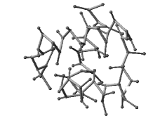
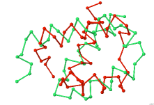
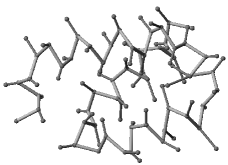
Figure 6: Protein 1ENH: native state (left), prediction—green/light gray — compared to original — red/dark grey— (center), prediction (right)

In Figure 6, we depict the native state (on the left) and our best prediction (on the right) for the protein 1ENH with the backbone and centroids. In the middle, we show the RMSD overlap of the $C_{\alpha}$ atoms between the native conformation (red/dark gray) and the prediction (green/light gray). The main features are preserved and only the right loop that connects the two helices appears to have moved significantly. This could be avoided by introducing a richer set of alternative fragments in that area and thus allow a more relaxed placement of the fragments.

An important issue is that it is not obvious that the reduced representation and the energy function used here are able to distinguish the native structure from decoys constructed to minimize that energy function. The straightforward comparison between RMSD and energy is not completely meaningful because the native structure should be energy-minimized before energy comparison. This can be noted by comparing the conformations obtained by enumeration and LNS. The model in use improves w.r.t. the $C\alpha$ model as presented in [Dal Palù et al. (2004)]. However, some fine tuning of the energy coefficients is still necessary in order to improve the correlation, while preserving the overall constraint model. This will be a further area of investigation. Our results show that the method can scale well and that further speed-up may be obtained by considering larger fragments as done by tools like Rosetta. Rosetta is in fact the state-of-the-art predictor tool (e.g., the small protein 1ENH is predicted by Rosetta in less than one minute with a RMSD of 4.2 Å).

6 Conclusions and future work

In this paper we presented the design and implementation of a constraint logic programming tool to predict the native conformation of a protein, given its primary structure. The methodology is based on a process of fragments assembly, using templates retrieved from a protein database, that is clustered according to shape similarity. We used templates based on sequences of 4 amino acids. The constraint solving process takes advantage of a large neighboring search strategy, which has been shown to be particularly effective when dealing with longer proteins.

The preliminary experimental results confirm the strong potential for this fragment assembly scheme. The proposed method has a significant advantage over schemes like Rosetta—the use of $CLP(\mathcal{FD})$ enables the simple addition of ad-hoc constraints and experimentation with different local search moves and energy functions. The implementation presented here constitutes a proof of principle.

In order to make this a useful tool in a realistic prediction scenario several improvements must be implemented. The choice of 4-residue fragment will be improved in the next future in two directions: fragments will be chosen based on sequence or profile alignment (rather than exact match) against a non-redundant representative set of sequences whose structure is known; the size of the fragment will be chosen based on the alignment and will not be restricted to 4-residues.

The reduced representation used here should be replaced by an all-atom representation at least for the backbone atoms whose hydrogen bonds define the proper relative arrangement of beta-strands not belonging to the same fragment. In general we plan to test different energy functions that better correlate with RMSD w.r.t. the (known) native structures and the computed ones. It is likely that with sequences longer than those considered here predictions will not be equally good in all parts of the molecule, therefore alternative measurements of similarity like GDT-TS [Zemla (2003)] might be more appropriate.

Other (possibly redundant) constraints and constraint propagation techniques should be analyzed, including the migration to the C++ solver Gecode.

Acknowledgments.

The work is partially supported by the grants: GNCS-INdAM Tecniche innovative per la programmazione con vincoli in applicazioni strategiche, PRIN 2007 Computer simulations of Glutathione Peroxidases: insights into the catalytic mechanism, PRIN 2008 Innovative multi-disciplinary approaches for constraint and preference reasoning, NSF HRD-0420407 and NSF IIS-0812267.

References

- Backofen and Will (2006) Backofen, R. and Will, S. 2006. A constraint-based approach to fast and exact structure prediction in three-dimensional protein models. Constraints 11, 1, 5–30.
- Barahona and Krippahl (2008) Barahona, P. and Krippahl, L. 2008. Constraint programming in structural bioinformatics. Constraints 13, 1-2, 3–20.
- Ben-David et al. (2009) Ben-David, M., Noivirt-Brik, O., Paz, A., Prilusky, J., Sussman, J. L., and Levy, Y. 2009. Assessment of CASP8 structure predictions for template free targets. Proteins: Structure, Function, and Bioinformatics 77, S9, 50–65.
- Berrera et al. (2003) Berrera, M., Molinari, H., and Fogolari, F. 2003. Amino acid empirical contact energy definitions for fold recognition in the space of contact maps. BMC Bioinformatics 4, 8.
- Crescenzi et al. (1998) Crescenzi, P., Goldman, D., Papadimitriou, C., Piccolboni, A., and Yannakakis, M. 1998. On the complexity of protein folding (extended abstract). In STOC ’98: Proceedings of the thirtieth annual ACM symposium on Theory of computing. ACM, New York, NY, USA, 597–603.
- Dal Palù et al. (2004) Dal Palù, A., Dovier, A., and Fogolari, F. 2004. Constraint logic programming approach to protein structure prediction. BMC Bioinformatics 5, 186.
- Dal Palù et al. (2007) Dal Palù, A., Dovier, A., and Pontelli, E. 2007. A constraint solver for discrete lattices, its parallelization, and application to protein structure prediction. Softw., Pract. Exper. 37, 13, 1405–1449.
- Dal Palù et al. (2010) Dal Palù, A., Dovier, A., and Pontelli, E. 2010. Computing approximate solutions of the protein structure determination problem using global constraints on discrete crystal lattices. Int. J. Data Min. Bioinformatics 4, 1, 1–20.
- Dotu et al. (2008) Dotu, I., Cebrián, M., Hentenryck, P., and Clote, P. 2008. Protein structure prediction with large neighborhood constraint programming search. In CP ’08: Proceedings of the 14th international conference on Principles and Practice of Constraint Programming. LNCS, vol. 5202. Springer-Verlag, Berlin, Heidelberg, 82–96.
- Fogolari et al. (2007) Fogolari, F., Pieri, L., Dovier, A., Bortolussi, L., Giugliarelli, G., Corazza, A., Esposito, G., , and Viglino, P. 2007. Scoring predictive models using a reduced representation of proteins: model and energy definition. BMC Structural Biology 7, 15.
- Levinthal (1968) Levinthal, C. 1968. Are there pathways in protein folding? J. Chim. Phys. 65, 44–45.
- Lovell et al. (2003) Lovell, S., Davis, I., Arendall, W., de Bakker, P., Word, J., Prisant, M., Richardson, J., and Richardson, D. 2003. Structure validation by cα geometry: , and cβ deviation. Proteins 50, 437–450.
- Raman et al. (2009) Raman, S., Vernon, R., Thompson, J., Tyka, M., Sadreyev, R., Pei, J., Kim, D., Kellogg, E., DiMaio, F., Lange, O., Kinch, L., Sheffler, W., Kim, B.-H., Das, R., Grishin, N. V., and Baker, D. 2009. Structure prediction for casp8 with all-atom refinement using rosetta. Proteins 77, S9, 89–99.
- Shaw (1998) Shaw, P. 1998. Using constraint programming and local search methods to solve vehicle routing problems. In CP ’98: Proceedings of the 14th international conference on Principles and Practice of Constraint Programming. LNCS, vol. 1520. Springer, 417–431.
- Wu et al. (2007) Wu, S., Skolnick, J., and Zhang, Y. 2007. Ab initio modeling of small proteins by iterative tasser simulations. BMC Biology 5, 17.
- Zemla (2003) Zemla, A. 2003. LGA: A method for finding 3D similarities in protein structures. Nucleic acids research 31, 13, 3370–3374.