Disordered spinor Bose-Hubbard model

Abstract

We study the zero temperature phase diagram of the disordered spin-$1$ Bose-Hubbard model in a 2-dimensional square lattice. To this aim, we use a mean field Gutzwiller ansatz and a probabilistic mean field perturbation theory. The spin interaction induces two different regimes corresponding to a ferromagnetic and antiferromagnetic order. In the ferromagnetic case, the introduction of disorder reproduces analogous features of the disordered scalar Bose-Hubbard model, consisting in the formation of a Bose glass phase between Mott insulator lobes. In the antiferromagnetic regime the phase diagram differs more from the scalar case. Disorder in the chemical potential can lead to the disappearance of Mott insulator lobes with odd integer filling factor and, for sufficiently strong spin coupling, to Bose glass of singlets between even filling Mott insulator lobes. Disorder in the spinor coupling parameter results in the appearance of a Bose glass phase only between the $n$ and $n+1$ lobes for $n$ odd. Disorder in the scalar Hubbard interaction inhibits Mott insulator regions for occupation larger than a critical value.

I Introduction

Spinor Bose-Hubbard (BH) models describe strongly correlated lattice systems where bosons have internal angular momentum whose orientation in space is not externally constrained. Bosonic interactions are sensitive to the spin degree of freedom leading to a rich variety of orderings in the ground state at zero temperature. In atomic gases, the spin degree of freedom corresponds to the manifold of degenerate -in absence of an external magnetic field- Zeeman energy states associated to a given hyperfine level $F$, i.e.  $\{|F,m_{F}\rangle\}$ where $m_{F}=-F,..,F$. In this context, we identify the spin of the atom with the hyperfine quantum number $F$. Like in the scalar case, ultracold atomic spinor interactions can be parametrised by two-body short range (s-wave) collisions. Due to the rotational symmetry, two-body collisions between atoms depend only on their total spin and not on its orientation. Moreover, symmetry arguments impose that the collisions between two identical bosons in a hyperfine spin level $F$ are restricted to total even spin $S=2F,2F-2,...,0$. Different properties of spinor condensates in a single trap has been discussed Ho (1998); Ohmi and Machida (1998); Law et al. (1998); Ho and Yip (2000). The confinement of the particles in a lattice leads to an enhancement of the interactions, pushing the system to a strongly correlated regime. As it happens in the scalar BH case Fisher et al. (1989), the competition between the different energy scales present in spinor BH models determines the ordering properties -quantum phases- of the ground state. Modifying the energy ratio between the hopping and interactions allows to cross a quantum phase transition between a spinor superfluid (SF) condensate and a Mott insulator (MI) state Imambekov et al. (2003); Tsuchiya et al. (2004); Rizzi et al. (2005).

The crucial effects of the disorder in condense matter systems were advanced in the seminal contribution of Anderson Anderson (1958), predicting an exponential localization of all energy eigenstates of a single particle in a periodic potential when additional impurities are added to it. It took several years to recognize the enormous consequences Anderson’s result had, but nowadays it is well established that disorder, and specifically quenched disorder (i.e. frozen during the typical time scales of the system), is an essential ingredient in condensed matter systems and related topics as conductivity, transport, high-Tc superconductivity, neural networks, insulating phases or quantum chaos to mention few examples (see Lewenstein et al. (2007) and references therein). Disorder is intrinsically difficult to treat firstly because, in order to characterize the system, one should average over different realizations of disorder which is usually a hard task. Secondly, disordered systems often develop a complex landscape of low energy states making the problem of minimization to find ground states very involved. Thirdly, they incorporate often fractal and ultrametric structures, all together making the problem of simulating quantum disordered systems a very complex one.

In recent years, it has become clear that ultracold atoms offer a new paradigm of disordered systems, due to the fact that random or quasi random disorder can be produced in these systems in a controlled and reproducible way. Standard methods to achieve such controlled disorder are the use of speckle patterns Horak et al. (1998); Boiron et al. (1999) which can be added to the confining potential, or optical superlattices created by the simultaneous presence of optical lattices of incommensurate frequencies Roth and Burnett (2003); Damski et al. (2003); Diener et al. (2001). Other methods include using an admixture of different atomic species randomly trapped in sites distributed across the sample and acting as impurities Gavish and Castin (2005); Massignan and Castin (2006), or the use of inhomogeneous magnetic fields which modify randomly, close to a Feshbach resonance, the scattering length of the atoms in the sample depending on their spatial position Gimperlein et al. (2005); Chin et al. (2010).

Strongly correlated bosons in a lattice in the presence of external random potentials were first considered in Fisher et al. (1989) where the phase diagram in the $t-\mu$ plane of the system, $\mu$ being the chemical potential, was worked out. The three possible ground states predicted were: (i) an incompressible MI with a gap for particle-hole excitations; (ii) a gapless Bose-glass (BG) insulator with finite compressibility and exponentially decaying superfluid correlations in space; and (iii) a SF phase with the usual off-diagonal long range order. Previously, the onset of superfluidity in a random potential in 1D was studied in Ma et al. (1986), considering hard core bosons and using a mean field theory including quantum fluctuations, and in Giamarchi and Schulz (1988), where a renormalization group approach was developed to study a one-dimensional system of interacting bosons in a random potential. In recent years it has been shown that the question of the simultaneous presence of disorder and interactions constitutes an important and complex many body problem that is still far from being well understood (for a review see Sanchez-Palencia and Lewenstein (2010)).

Here we address the effects of disorder in the strongly interacting spin-$1$ BH model in two dimensions (2D). For spin-$1$ systems, the short range two body collisions lead to a spin independent effective coupling strength $U_{0}$, similar to the scalar case, plus the spinor coupling $U_{2}$. With the help of a Gutzwiller ansatz, supplemented by a perturbative mean field approach, we provide the phase diagram on different regimes of the phase space determined by a spinor coupling and the disorder. The Gutzwiller mean field approach is known to give reasonable results for the scalar and the spin-$1$ SF-MI transition in 2D Tsuchiya et al. (2004). It has also been used to signal in the presence of disorder, a BG phase in ultracold scalar bosonic gases Damski et al. (2003) as well as diverse glassy phases in Bose-Fermi mixtures Ahufinger et al. (2005). A Gutzwiller mean field approach yield to correct ground state for small values of the spinor coupling, since it neglects correlations between different sites and thus is not precise enough in determining accurately the boundaries between distinct quantum phases. Nonetheless it provides a valuable estimate on the physics of the system and permits easily to include the effects of disorder going beyond the homogeneous mean field approach.

One may argue that the mean field approach could work even better in the three dimensional case. However, the necessarily inhomogeneous, disordered systems are then much harder to treat being computationally very demanding. For that reason we restrict ourselves to the 2D case only as in the earlier studies Damski et al. (2003); Sanpera et al. (2004); Ahufinger et al. (2005).

Our main results can be summarized as follows. In the non disordered case, and for $U_{2}>0$, we confirm previous findings Tsuchiya et al. (2004); Imambekov et al. (2003); Kimura et al. (2006) consisting in: (i) a first (second) order phase transition from MI to SF for even (odd) occupation numbers in the region $U_{2}/U_{0}<u_{c}$ (with $u_{c}\simeq 0.2$) and $t\ll U_{2}$, where $t$ denotes the hopping; (ii) a second order phase transition from even occupation MI lobes to SF if $U_{2}/U_{0}>u_{c}$. In the presence of disorder in the chemical potential the above effects, (i) and (ii), persist together with the appearance of a BG phase between the MI lobes. For $U_{2}/U_{0}>0.5$, odd occupation MI lobes disappear while even lobes survive and the corresponding BG is formed only by singlets between the remaining lobes. Also disorder can make the odd occupation MI lobes to disappear but the BG phase is nematic if $U_{2}/U_{0}<0.5$. Assuming disorder in the $U_{2}$ coupling we observe that the BG phase appears only between every second pair of lobes and we explain such a peculiar behaviour using perturbation theory in the vanishing tunneling limit. On the other hand, disorder on the spinless term of the interaction coupling reproduces qualitatively the results found for scalar gases Gimperlein et al. (2005).

The paper is organized as follows: In section II we introduce the spin-1 BH model and shortly review the different phases in the homogeneous case (without disorder). In Sec. II.1 we discuss first the exact phase diagram in the absence of tunneling to grasp the features of the MI phase. In Sec.II.2 we comment the perturbative results for small tunneling, while in II.3 and II.4 we derive a mean field phase diagram for finite tunneling using both, mean field perturbation theory (MFPT) and Gutzwiller mean field approach. In section III we analyze in detail the effects of disorder. Two types of disorder are considered here, disorder on the on-site energies, resulting from a random external potential, and disorder on the interactions both on the scalar and the explicit spin dependent part. We calculate the phase diagram in the disordered case using both, a Gutzwiller ansatz and MFPT. Finally, in Sec. IV we present our concluding remarks and open questions.

II Bose-Hubbard model for spin-1 bosons

Low energy spin-1 bosons loaded in optical lattices sufficiently deep so that only the lowest energy band is relevant can be described by the spinor BH model. The corresponding Hamiltonian is Imambekov et al. (2003):

$$\hat{H} = -t\sum_{\left\langle i,j\right\rangle,\sigma}\left(\hat{a}_{i\sigma}^{\dagger}\hat{a}_{j\sigma}+\hat{a}_{j\sigma}^{\dagger}\hat{a}_{i\sigma}\right)+\frac{U_{0}}{2}\sum_{i}\hat{n}_{i}(\hat{n}_{i}-1)$$ (1)

$$+ \frac{U_{2}}{2}\sum_{i}\left(\hat{\mathbf{S}}_{i}^{2}-2\hat{n}_{i}\right)-\mu\sum_{i}\hat{n}_{i},$$

where $\left\langle i,j\right\rangle$ indicates that the sum is restricted to nearest neighbors in the lattice and $\hat{a}_{i\sigma}^{\dagger}$ ($\hat{a}_{i\sigma}$) denotes the creation (annihilation) operator of a boson in the lowest Bloch band localized on site $i$ with spin component $\sigma=0,\pm 1$.

The first term in (1) represents the kinetic energy and describes spin symmetric hopping between nearest-neighbor sites with site independent tunneling amplitude $t$. The second and third term account for spin independent and spin dependent on site interactions, respectively. These energies at site $i$ are defined as $U_{0,2}=c_{0,2}\int d\vec{r}w^{4}(\vec{r}-\vec{r}_{i})$ with $c_{0}=4\pi\hbar^{2}(a_{0}+2a_{2})/3m$ and $c_{2}=4\pi\hbar^{2}(a_{2}-a_{0})/(3m)$, where $a_{S}$ is the s-wave scattering length corresponding to the channel with total spin $S$ Ho (1998); Ohmi and Machida (1998) and $w(\vec{r}-\vec{r}_{i})$ is the Wannier function of the lowest band at site $i$. While the second term of (1) is spin independent and equivalent to the interaction energy for scalar bosons, the third term represents the energy associated with spin configurations within lattice sites with

$$\hat{\mathbf{S}}_{i}=\sum_{\sigma\sigma^{\prime}=0,\pm 1}\hat{a}^{\dagger}_{\sigma i}\vec{F}_{\sigma\sigma^{\prime}}\hat{a}_{\sigma^{\prime}i},$$ (2)

being the spin operator at site $i$ and $\vec{F}$ the traceless spin-1 matrices. The explicit form of the spin operator $\hat{\mathbf{S}}_{i}$ reads

$$\hat{S}_{z} = \hat{n}_{1}-\hat{n}_{-1}$$

$$\hat{S}_{x} = \frac{1}{\sqrt{2}}\left[\left(\hat{a}_{1}^{\dagger}+\hat{a}_{-1}^{\dagger}\right)\hat{a}_{0}+H.c.\right]$$

$$\hat{S}_{y} = \frac{i}{\sqrt{2}}\left[\left(-\hat{a}_{1}^{\dagger}+\hat{a}_{-1}^{\dagger}\right)\hat{a}_{0}-H.c.\right].$$ (3)

$\hat{\mathbf{S}}$’s components obey standard angular momentum commutation relations $[\hat{S}_{l},\hat{S}_{j}]=i\epsilon_{ljk}\hat{S}_{k}$. Note that the spin-interaction term favors a configuration with total magnetization zero (denoted as polar and sometimes antiferromagnetic) for $U_{2}>0$ and ferromagnetic for $U_{2}<0$ Ho (1998); Ohmi and Machida (1998); Law et al. (1998). In the grand canonical approach the total number of particles is controlled by the last term of (1) where $\mu$ is the chemical potential and

$$\hat{n}_{i}=\sum_{\sigma=0,\pm 1}\hat{n}_{i,\sigma},$$ (4)

is the total number of bosons on site $i$. Hamiltonian (1) can be straightforwardly derived from the microscopical description of bosonic atoms, with a hyperfine spin $F=1$, loaded in a deep optical lattice and considering the two-body short range (s-wave) collisions. More details about the derivation can be found in Jaksch et al. (1998); Ho (1998); Ohmi and Machida (1998); Koashi and Ueda (2000); Tsuchiya et al. (2004).

Notice also that, since the orbital part of the wave function in one lattice site is the product of Wannier functions for all the atoms, it is symmetric under permutation of any two atoms. Therefore, the spin part of the wavefunction should also be symmetric due to Bose statistics. This imposes $S_{i}+n_{i}$ to be even Wu (1996), being $S_{i}$ and $n_{i}$ the quantum numbers labelling the eigenvalues of $\hat{\mathbf{S}}_{i}$ and $\hat{n}_{i}$.

As in the scalar case, the spinor BH system exhibits a quantum phase transition between superfluid and insulating states Imambekov et al. (2003); Tsuchiya et al. (2004). In the insulating states, fluctuations in the atom number per site are suppressed and virtual tunneling gives rise to effective spin exchange interactions that determine a rich phase diagram in which different insulating phases differ by their spin correlations. The appearance of spin mediated tunneling transitions in the optical lattice depends clearly on the ratio between the different energy scales appearing on the BH Hamiltonian (1). In alkalins, the scattering lengths are such that spin-independent interactions $U_{0}$ are larger than spin-dependent ones $U_{2}$. In such case the SF-MI transition depends mostly on the ratio $t/U_{0}$. However, inside the insulating regime, the value of $U_{2}$ plays an important role if $U_{2}\geq t$ where it competes with the spin-exchange interactions induced by small fluctuations of the particle number determining the spin structure. On the contrary, if $t\gg U_{2}$ tunneling acts similarly for all spin components and the gas will behave as a strongly correlated scalar gas.

II.1 The phase diagram at $t=0$.

To better understand the effects of spin mediated interactions when disorder is present let us first summarize the phase diagram at $t=0$ (atomic limit) without disorder. In this limit, the Hamiltonian reduces to the sum of independent single-site Hamiltonians $\hat{H}_{0}=\sum_{i}\hat{H}_{0,i}$ with

$$\hat{H}_{0,i}=-\mu\hat{n}_{i}+\frac{U_{0}}{2}\sum_{i}\hat{n}_{i}(\hat{n}_{i}-1)+\frac{U_{2}}{2}\sum_{i}\left(\hat{\mathbf{S}}_{i}^{2}-2\hat{n}_{i}\right).$$ (5)

Since $\left[\hat{n}_{i},\hat{\mathbf{S}}_{i}^{2}\right]=0$, the eigenstates of the single site Hamiltonian can be labeled by three quantum numbers $\left|S_{i},m_{i};n_{i}\right\rangle$, such that:

$$H^{0}_{i}\left|S_{i},m_{i};n_{i}\right\rangle=E_{0}(S_{i},n_{i},U_{0},U_{2},\mu)\left|S_{i},m_{i};n_{i}\right\rangle$$ (6)

with:

$$E_{0}(S_{i},n_{i},U_{0},U_{2},\mu) = -\mu n_{i}+\frac{1}{2}U_{0}n_{i}(n_{i}-1)$$ (7)

$$+ \frac{1}{2}U_{2}\left[S_{i}(S_{i}+1)-2n_{i}\right].$$

From Eq.(7), one can deduce the structure of the ground state of the insulator phases in the limit $t=0$. For antiferromagnetic interactions, $U_{2}>0$, the minimum energy $E^{min}_{0}$ is attained with minimum $S_{i}$, its specific value depending of the number of atoms per site. Thus, for even filling factor, the minimum spin is zero and the state is described as $\left|0_{i},0_{i};n_{i}\right\rangle$ with $n_{i}$ even. This state is known as spin singlet insulator Demler and Zhou (2002). If the atom number per site is odd, then the minimum spin per site is one and the state reads $\left|1_{i},m_{i};n_{i}\right\rangle$. The chemical potential region for which each of the two phases are the ground states can be found easily from Eq.(7):
(i) MI with $n$ odd and spin $1$ on each lattice site is the ground state if $E_{0}(1,n)<E_{0}(0,n-1)$ and $E_{0}(1,n)<E_{0}(0,n+1)$ i.e. when $(n-1)U_{0}<\mu<nU_{0}-2U_{2}$. This sets an upper bound on the spin coupling $U_{2}/U_{0}\leq 0.5$ above which the odd lobes cease to exist Demler and Zhou (2002).
(ii) MI with $n$ even and spin $0$ on each site are ground states if $E_{0}(0,n)<E_{0}(1,n-1)$ and $E_{0}(0,n)<E_{0}(1,n+1)$ leading to $(n-1)U_{0}-2U_{2}<\mu<nU_{0}$ for $U_{2}/U_{0}\leq 0.5$. For higher values, odd lobes do not exist and the stability conditions read $E_{0}(0,n)<E_{0}(0,n-2)$ and $E_{0}(0,n)<E_{0}(0,n+2)$. The last two conditions set an $n$-dependent upper bound on the maximum value of $U_{2}/U_{0}\leq(n+1/2)$.
The ferromagnetic side of the diagram is easily calculated imposing an integer number of particles and realising that the minimisation of the energy implies maximum spin value i.e. $S_{i}=n_{i}$.

The exact phase diagram in the ($U_{2}/U_{0},\mu/U_{0}$) plane is displayed in Fig. 1 providing the width of the MI lobes at $t=0$ as a function of $U_{2}/U_{0}$. It is interesting to note that the right boundary of even lobes in the range $0<U_{2}/U_{0}<0.5$ does not change with $U_{2}$. This fact leads to a stability with respect to disorder in this parameter, as we shall show in the Sec. III.3, corresponding to the absence of the BG phase between lobes with occupation $n$ and $n+1$ with $n$ even in the presence of disorder in $U_{2}$. In the antiferromagnetic region, for $U_{2}$ large enough, odd lobes disappear while even lobes broaden. In the ferromagnetic case the lobes shrink as $|U_{2}|$ increases and disappear for $U_{2}=-1$.

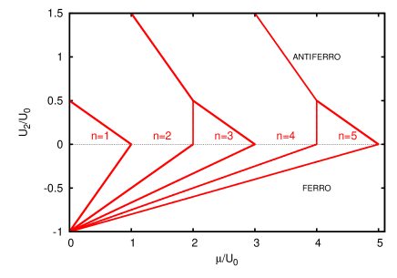
Figure 1: Phase diagram of the spinor $F=1$ BH model in the limit $t=0$. Each region corresponds to a MI phase with a different occupation number.

II.2 Perturbative approach for small $t$

For small but finite tunneling $t/U_{0}$ and $|U_{2}|/U_{0}\ll 1$, it is possible to perform perturbation theory and derive an effective Hamiltonian to second order in $t/U_{0}$ Imambekov et al. (2003), that permits to study insulating phases. The explicit form of the effective second order perturbation Hamiltonian depends on the number of bosons per site, odd or even. A mean field theory with a product state ansatz, applied to the effective Hamiltonian provides the following character of insulating states for the low $t$ limit. For $U_{2}<0$ the MI lobe with $n$ bosons is ferromagnetic with $S=n$. The situation is richer for antiferromagnetic ordering and depends on the dimension of the system.

We restrict ourselves to 2D systems and revise the results from Imambekov et al. (2003). The MI lobes for odd $n$ are in a nematic phase characterized by zero expectation value of all the spin components but broken spin symmetry $\left<S_{iz}^{2}\right>=0$ and $\left<S_{ix}^{2}\right>=\left<S_{iy}^{2}\right>=1$ (nematic phase for 3D spin systems has been studied also in Chen and Levy (1973); Papanicolaou (1988)). The corresponding state is well described by the mean field ansatz $|\psi\rangle=\prod_{i}|S_{i}=1,m_{i}=0\rangle$. For $n$ even (even MI lobes) and sufficiently large $U_{2}$, the spin-dependent term in the Hamiltonian dominates and a singlet configuration $|\psi\rangle=\prod_{i}|S_{i}=0,m_{i}=0\rangle$ is realized. However, when $t^{2}\propto U_{0}U_{2}$ tunneling may effectively couple $S=0$ and $S=2$ states leading again to a nematic state. As shown in Imambekov et al. (2003), a first order transition may turn place within the MI lobe between the singlet configuration (for low $t$) and the nematic state (at higher $t$ values) with a critical tunnelling rate fulfilling $zt_{c}^{2}=0.5U_{2}U_{0}$ for $n=2$ where $z$ is the number of neighbors. Such phase transition may take place only if $t_{c}$ is sufficiently small so that the MI lobe exists at this value, otherwise a singlet MI - SF phase transition occurs first and the nematic state may not be formed.

II.3 Standard Mean Field Perturbative Approach

The MI-SF transition for spin-$1$ has also been studied using standard mean field perturbative approach by Tsuchiya et al. Tsuchiya et al. (2004). We describe these results in more detail since they are a starting point for our study of the effects of disorder. Neglecting second order fluctuations of the bosonic annihilation and creation operators we obtain the condition $(\hat{a}^{\dagger}_{i,\sigma}-\langle{\hat{a}_{i,\sigma}}\rangle)(\hat{a}_{j,\sigma}-\langle{\hat{a}_{j,\sigma}}\rangle)\simeq 0$ which allows to decouple the hopping term as $\hat{a}^{\dagger}_{i\sigma}\hat{a}_{j\sigma}\simeq\psi^{*}_{i\sigma}\hat{a}_{j\sigma}+\hat{a}^{\dagger}_{i\sigma}\psi_{j\sigma}-\psi^{*}_{i\sigma}\psi_{j\sigma}$, where we have introduced the superfluid order parameter $\psi_{j\sigma}=\langle{\hat{a}_{j\sigma}}\rangle$ which, in a homogeneous lattice, is site-independent. The Hamiltonian reduces now to a sum of local terms $\hat{H}_{MF}=\sum_{i}\hat{h}_{i}$ with

$$\hat{h} = -tz\sum_{\sigma}\left[\left(\psi_{\sigma}\hat{a}_{\sigma}^{\dagger}+\psi_{\sigma}^{*}\hat{a}_{\sigma}\right)-\left|\psi_{\sigma}\right|^{2}\right]-\mu\hat{n}$$ (8)

$$+ \frac{U_{0}}{2}\hat{n}(\hat{n}-1)+\frac{U_{2}}{2}\left(\hat{\mathbf{S}}^{2}-2\hat{n}\right),$$

where the site index $i$ has been dropped since we are considering here an homogeneous system, and $z$ denotes the number of nearest neighbours. The superfluid order parameter $\psi_{\sigma}$ has to be determined by minimizing the free energy $f=-1/\beta\log{\mathrm{T}r}\left[\exp{(-\beta\hat{h})}\right]$, where $\beta=1/K_{B}T$ being $K_{B}$ the Boltzmann’s constant and $T$ the temperature. Here, since we are interested only at the zero-temperature properties, the former condition reduces to the minimization of the ground state energy $E_{GS}(\psi_{\sigma})=\left\langle GS\right|\hat{h}\left|GS\right\rangle$ with the self-consistent condition $\left\langle GS\right|\hat{a}_{\sigma}\left|GS\right\rangle=\psi_{\sigma}$. For sufficiently small $t$ we can apply perturbation theory, $\hat{h}=\hat{H}_{0}+\hat{V}(t)$, and use as a basis the eigenstates of $\hat{H}_{0}$ (7). The perturbation term is given by

$$\hat{V}=-tz\sum_{\sigma}\left[\left(\psi_{\sigma}\hat{a}_{\sigma}^{\dagger}+\psi_{\sigma}^{*}\hat{a}_{\sigma}\right)-\left|\psi_{\sigma}\right|^{2}\right].$$ (9)

Let us focus on the antiferromagnetic case $U_{2}>0$. A tedious but straightforward calculation of the matrix elements of the perturbation leads to the phase boundaries between the SF phase and the MI phase in the $(\mu/U_{0},t/U_{0}$) plane for a given value of the $U_{2}/U_{0}$ coupling. Notice that being $\hat{V}\propto(\hat{a}_{\sigma}^{\dagger}+\hat{a}_{\sigma})$ only even terms on the perturbation expansion survive. As derived in Tsuchiya et al. (2004) the ground-state energy up to second order is for odd occupation number given by:

$$E^{(2)}(S=1,n,t,U_{0},U_{2},\mu,\psi_{\sigma})=$$ (10)

$$= zt\left[1-zt\sum_{j=1,4}\alpha_{j}(n,U_{0},U_{2},\mu)\right]\sum_{\sigma}\left|\psi_{\sigma}\right|^{2},$$

and for even occupation

$$E^{(2)}(S=0,n,t,U_{0},U_{2},\mu,\psi_{\sigma})=$$ (11)

$$= zt\left[1-\frac{zt}{3}\sum_{j=1,2}\gamma_{j}(n,U_{0},U_{2},\mu)\right]\sum_{\sigma}\left|\psi_{\sigma}\right|^{2},$$

with

$$\alpha_{1}(n,U_{0},U_{2},\mu) = \frac{n+2}{3\delta_{n-1,0;n,1}(U_{0},U_{2},\mu)},$$

$$\alpha_{2}(n,U_{0},U_{2},\mu) = \frac{4(n-1)}{15\delta_{n-1,2;n,1}(U_{0},U_{2},\mu)},$$

$$\alpha_{3}(n,U_{0},U_{2},\mu) = \frac{n+1}{3\delta_{n+1,0;n,1}(U_{0},U_{2},\mu)},$$

$$\alpha_{4}(n,U_{0},U_{2},\mu) = \frac{4(n+4)}{15\delta_{n+1,2;n,1}(U_{0},U_{2},\mu)},$$ (12)

$$\gamma_{1}(n,U_{0},U_{2},\mu) = \frac{n+3}{\delta_{n+1,1;n,0}(U_{0},U_{2},\mu)},$$

$$\gamma_{2}(n,U_{0},U_{2},\mu) = \frac{n}{\delta_{n-1,1;n,0}(U_{0},U_{2},\mu)},$$ (13)

and $\delta_{l,r;n,s}(U_{0},U_{2},\mu)=E_{0}(l,r,U_{0},U_{2},\mu)-E_{0}(s,n,U_{0},U_{2},\mu)$. Minimisation of the energy for a finite order parameter (corresponding to SF) is achieved when the expressions on the parenthesis in (10) and (11) are negative. On the contrary, the MI phase, corresponding to zero order parameter is associated to a positive value of such expressions. Hence, the phase boundaries between the SF and the MI in the $(\mu/U_{0},t/U_{0})$ plane, for a given value of the spin interaction $U_{2}$ are given by:

$$t_{odd}=\frac{1}{z\sum_{j=1,4}\alpha_{j}(n,U_{0},U_{2},\mu)}$$ (14)

$$t_{even}=\frac{3}{z\sum_{j=1,2}\gamma_{j}(n,U_{0},U_{2},\mu)}$$ (15)

Notice also that the dimensionality of the lattice is included through the parameter $z$ which indicated the number of nearest neighbours.

The analysis of the ferromagnetic regime ($U_{2}<0$) can be done in the same way imposing the condition $S=n$. Since in this case all the spins are aligned, we can consider only one of the components $m=\pm S$ in the perturbative expansion. A straightforward calculation leads to the following explicit expression for the MI to SF boundary:

$$t_{ferro}=-\frac{\left(n+nU_{2}-\mu\right)\left[(-1+n)\left(1+U_{2}\right)-\mu\right]}{z\left(1+U_{2}+\mu\right)}.$$ (16)

II.4 Variational Gutzwiller approach

The variational Gutzwiller approximation is a non perturbative approach, where the wave function takes a form of a product over all $M$ sites of the lattice

$$\left|\psi\right\rangle=\prod_{i=1}^{M}\sum_{n=0}^{n_{max}}g_{i}(n)\sum_{S=0}^{n}f_{i}(S,n)\sum_{m=-S}^{S}h_{i}(S,m,n)\left|S,m,n\right\rangle_{i}$$ (17)

where $g_{i},\ h_{i},\ f_{i}$ are the variational coefficients to be determined by minimizing the BH Hamiltonian (1) with the above ansatz. That implies decoupling in the tunneling term $\langle\hat{a}_{i\sigma}^{\dagger}\hat{a}_{j\sigma}\rangle=\hat{n}_{i\sigma}\delta_{ij}+\langle\hat{a}_{i\sigma}^{\dagger}\rangle\langle\hat{a}_{j\sigma}\rangle(1-\delta_{ij})$. Observe that for consistency of notation we should rather use $\psi_{i\sigma}$ instead of $\langle\hat{a}_{j\sigma}\rangle$. The Gutzwiller variational state is a product state of on-site wave functions so it cannot reproduce intersite correlations or entanglement between different sites. Being a generalisation of the standard mean field approximation, the Gutzwiller ansatz is expected to be exact in the limit of infinite dimensions. To mark the limits between the SF and MI phases in the Gutzwiller approach, we recall that the MI phase prevails for small hopping amplitude and it is characterized by a finite gap in the spectrum and zero compressibility defined as $\kappa=\frac{\partial\rho}{\partial\mu}$ with

$$\rho=\frac{1}{N}\left\langle\sum_{j}\hat{n}_{j}\right\rangle,$$ (18)

and $N$ the total number of bosons. On the contrary, in the SF phase bosons are delocalized and a current flow is possible. This phase is characterized by a finite compressibility, gapless excitations and off-diagonal long range order accompanied by a non vanishing order parameter. Since the order parameter is not directly measurable, it is important to define experimental observable quantities marking the SF phase. These are typically the superfluid fraction $\rho_{S}$ and the condensate fraction $\rho_{C}$ Roth and Burnett (2003) (although it has been proposed recently the measure of the compressibility directly Delande and Zakrzewski (2009)). The superfluid fraction can be evaluated imposing a phase gradient in the tunneling corresponding to a current flow while the condensate fraction is defined as the highest eigenvalue of the one particle density matrix Roth and Burnett (2003); Damski et al. (2003). In an homogeneous case the site dependence can be omitted. It is measured experimentally by means of an interference density pattern giving coherent peaks in the SF phase Greiner et al. (2002). Notice that in the mean field approach, and so in the Gutzwiller ansatz, the condensed fraction decouples and both quantities, superfluid fraction and condensed fraction are related to the average $\psi_{\sigma}=\left\langle\hat{a}_{\sigma j}\right\rangle$, that can be taken as the order parameter, its value being zero in the MI phase and finite in the SF.

In Figure 2 we display the $\rho_{C}$ calculated both with the Gutzwiller ansatz and with the perturbation mean field approach (14-15) (solid line) for different values of the parameter $U_{2}/U_{0}$ (left column). Observe the different behavior between odd and even lobes (as described in the previous section). With increasing values of $U_{2}$, the even lobes start to dominate while the odd lobes shrink. We have checked numerically that for $U_{2}=0.5U_{0}$ the odd MI lobes disappear, in agreement with the $t=0$ predictions of the previous section. For small $U_{2}/U_{0}$ ratios, there exist a discrepancy between the perturbative mean field and Gutzwiller predictions for the boundaries of the even lobes already reported in Kimura et al. (2005). This discrepancy is correlated with the character of MI-SF transition as visualized in the right column of Fig. 2, where the condensate fraction is shown for selected $\mu=const$ lines corresponding to the tips of the lobes in the corresponding phase diagram.

For $U_{2}/U_{0}\leq 0.1$ (Fig. 2 first and second row) the condensate fraction is continuous across the phase transition for odd lobes (corresponding to second order phase transition) while it reveals a discontinuous jump, characteristic of the first order phase transition for even lobes. For $U_{2}/U_{0}\geq 0.3$ (Fig. 2 bottom row) only second order SF-MI transitions from both odd and even lobes are observed. In between these values it is not easy to characterize the order of the phase transition. An exhaustive numerical analysis shows that the value where the transition passes from first to second order is approximately $U_{2}/U_{0}=u_{c}\simeq 0.2$.

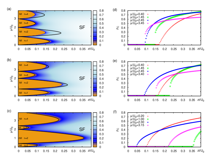
Figure 2: (Color online). Left panels depict the condensate fraction $\rho_{C}$ obtained numerically by the Gutzwiller ansatz for, (a)$U_{2}/U_{0}=0.02$, (b)$U_{2}/U_{0}=0.1$ and (c)$U_{2}/U_{0}=0.3$, in the homogeneous case without disorder, where MI lobes correspond to vanishing $\rho_{C}$ (orange areas). The lobes are compared with the boundaries obtained with the MFPT (solid lines). In the right panels is depicted $\rho_{C}$ as a function of $zt/U_{0}$ for values of $\mu/U_{0}$ corresponding to the lobes’ tips. In the transition between the MI and SF on the tip one can observe a first order transition for the even occupation lobes in panels (d) and (e) (abrupt jump on the condensate fraction) while for lobes corresponding to odd occupation the transition is always of the second order.

The observation of a first order phase transition in the even lobes - where MI is formed by singlets on each site- is not new and has been also pointed out in the mean field analysis of Tsuchiya et al. (2004); Kimura et al. (2005) in 2D, as well as in Quantum Monte Carlo (QMC) calculations Batrouni et al. (2009) in 1D. Recall also that another first order transition between singlet and nematic phases has been predicted within the MI lobes Imambekov et al. (2003) by using a restricted MF ansatz in the effective perturbative Hamiltonian.

Looking at the state provided by the Gutzwiller ansatz near the even lobes’ tips (Fig. 3), we observe that in the MI only the $S=0$ component is relevant, while in the SF phase the state becomes a linear combination of $f(S=2,n)|S=2,m=0,n\rangle+f(S=0,n)|S=0,m=0,n\rangle$ with $|f(S=2,n)|^{2}+|f(S=0,n)|^{2}$ close to $1$. A close inspection of the coefficients of the Gutzwiller ansatz (17) shows that, for $U_{2}/U_{0}<0.1$, $f(S=2,n)$ assumes a finite value abruptly (see Fig.3 (a) (b) (c)). Both states tend to contribute equally in the limit case in which $U_{2}=0$ (scalar case). Notice that this is also the origin of the discrepancy with the MFPT result where only states with $S=0$ are taken into account in the energy corrections. Even if we find that, in the MI, the state is singlet, the second order phase transition indicates a metastability inside the lobe of a nematic phase. A rough explication of this effect can be made for the lobe corresponding to $n=2$, noticing that a configuration with $S=2$ starts to become favorable when the kinetic energy becomes comparable with $E_{0}(S=2,n)-E_{0}(S=0,n)=3U_{2}$, so for $zt_{1}\simeq 6U_{2}$. This value can be compared with the MI tips obtained in the MFPT $zt_{2}=(U_{0}+2U_{2})\left[(2n+3)-\sqrt{4n^{2}+12n}\right]$. If $t_{1}<t_{2}$ the kinetic energy reduces the lobe with respect to the MFPT prediction and, as soon as the metastable nematic state becomes stable, SF phase appears discontinuously. On the other hand, if $t_{2}<t_{1}$ the system becomes SF before the appearance of the $S=2$ contribution and the MI-SF transition is smooth. It is easy to verify that $t_{1}\simeq t_{2}$ for $U_{2}/U_{0}\simeq 0.145$ which is not too far from the $u_{c}\simeq 0.2$ mentioned above. In contrast, for $U_{2}/U_{0}>u_{c}$ Gutzwiller and MFPT approaches coincide and effectively the contribution of the state $S=2$ is irrelevant close to the tip of the lobe (see Fig.3 (d)) and the transition rather than a phase crossing becomes again a second order phase transition.

Figure 3: Coefficients $|f(S=0,n=2)|^{2}$ (triangles) and $|f(S=2,n=2)|^{2}$ (squares) of the Gutzwiller state (17) as a function of $zt/U_{0}$. The value $\mu$ corresponds to the $n=2$ MI lobe’s tip. The panels refer to different values of spin interaction: $U_{2}/U_{0}=0.01$(a), $0.02$(b), $0.1$(c) and $0.3$(d).

III Disorder in Spinor Bose-Hubbard Model

As discussed in the introduction, the presence of disorder in the BH model allows, apart from MI, for another insulating phase, the BG phase. The characteristics of the phase diagram depend on the way the disorder is introduced. Here we will study the effect of two different kinds of disorder: disorder in $\mu$ (Sec. III.2), and disorder in the interactions $U_{2}$ and $U_{0}$ (Sec. III.3).

Diagonal disorder can be taken into account by adding to the Hamiltonian (1) a local term such

$$\hat{H}_{D}=\hat{H}+\sum_{i}\hat{H}_{dis}(\epsilon_{i})$$ (19)

where $\epsilon_{i}$ is a random variable defined for every site $i$ with a given probability distribution $p(\epsilon)$. While, depending on the origin of the disorder, different $p(\epsilon)$ may be considered (see e.g. Delande and Zakrzewski (2009)). Here we consider the simplest uniform distribution with $-\Delta\leq\epsilon_{i}\leq\Delta$ and the cases in which the disorder is equivalent to add a random term to one of the variables $\mu$, $U_{2}$ or $U_{0}$.

Notice that the addition of a site dependent disorder introduces inhomogeneity into the system. Thus, neither the mean field nor the Gutzwiller ansatz reduce to a “single site” effective Hamiltonian. Instead, the mean fields as well as Gutzwiller wave function coefficients become explicitly site dependent.

A Stochastic Mean Field Theory (SMFT), taking into account the inhomogeneity of $\psi_{i\sigma}$, has been proposed in Bissbort and Hofstetter (2009) for the scalar BH. Here we present a more simple MF theory, being a limiting case of SMFT, and compare it with the phase diagram obtained with the Gutzwiller ansatz. Good agreement for the MI boundaries has been found, as in the non disordered case, while the BG can be seen only by the Gutzwiller ansatz.

III.1 Probabilistic Mean Field approach

A first estimation of the MI lobes in the presence of disorder can be obtained by a MFPT, as described in the previous section. The generalization to the disordered case is not straightforward since, as we mentioned, the translational invariance is broken and the order parameter should be associated to a random variable $\psi_{j\sigma}$ defined for each site, with a certain probability distribution $P(\psi_{j\sigma})$. Nevertheless, since the disorder is assumed to be homogeneous on the lattice, we can introduce a simplified MFPT theory taking an average order parameter $\bar{\psi}_{\sigma}=\int d\psi_{j\sigma}P(\psi_{j\sigma})\psi_{j\sigma}$. In doing so, we are neglecting the classical fluctuations of the order parameter induced by the disorder. The self-consistent condition reads $\bar{\psi}_{\sigma}=\overline{\langle{\hat{a}_{i,\sigma}}\rangle}$, where the overbar indicates an ensemble average over the lattice. It is also equivalent, due to the self-averaging properties of the system, to an average over the random distribution. So the structure of the single-site mean field Hamiltonian remains the same, providing that one of the parameters changes according to $\nu\rightarrow\nu+\epsilon_{j}$, where, for a diagonal disorder, $\nu$ can be $\mu$, $U_{2}$ or $U_{0}$.

The minimization of the average ground-state energy which, up to second order corrections, reads

$$\bar{E}(s,n,t,U_{0},U_{2},\mu,\bar{\psi}_{\sigma}) = \bar{E}_{0}(s,n,U_{0},U_{2},\mu)$$

$$+ \bar{E}^{(2)}(s,n,t,U_{0},U_{2},\mu,\bar{\psi}_{\sigma}),$$

determines if $\bar{\psi}_{\sigma}$ is finite or zero. Notice that, since we are neglecting the fluctuations on the order parameter, a vanishing $\bar{\psi}_{\sigma}$ always corresponds to a MI phase, while BG cannot be detected, since it has $\bar{\psi}_{\sigma}=0$ but finite fluctuations. A more complete analysis needs a more complex theory, such as the SMFT Bissbort and Hofstetter (2009); Bissbort et al. (2010) where fluctuations are taken into account and $P(\psi_{j\sigma})$ is determined self-consistently.

In our simplified stochastic approach the MI-SF boundary is calculated using the equations for the MI boundaries (14) and (15) but using the averaged values $\bar{\alpha}_{j}$ and $\bar{\gamma}_{j}$ instead of $\alpha_{j}$ and $\gamma_{j}$.

III.2 Disorder in $\mu$

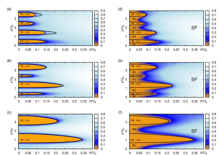
Figure 4: (Color online). Left column panels report the average density fluctuations $\sqrt{\overline{n^{2}}-\overline{n}^{2}}$ obtained from the Gutzwiller MF approach. MI lobes, corresponding to vanishing fluctuations (orange areas), are compared with the probabilistic mean field prediction (solid lines). Right column panels show the corresponding condensate fraction in comparison with the Gutzwiller MI lobes (solid lines). The zero-condensate fraction areas (orange areas) outside the MI lobes correspond to BG phase. For all panels, random disorder in the chemical potential with $\Delta=0.3U_{0}$ is considered. The different panels correspond $U_{2}/U_{0}=0.02$ (a-d), $U_{2}/U_{0}=0.1$ (b-e) and $U_{2}/U_{0}=0.3$ (c-f). Observe the disappearance of the odd filling MI lobes for the largest $U_{2}/U_{0}$ ratio in agreement with the simple estimate given in text.

We consider first the disorder in the chemical potential corresponding to $\hat{H}_{dis}(\epsilon_{i})=\epsilon_{i}\hat{n}_{i}$. To study the phase diagram, we use the Gutzwiller approach with a lattice large enough that self-averaging over the possible disorder realizations is already realized. Now we have to distinguish between three phases: SF, MI and BG. As before the (disorder averaged) condensate fraction helps to find the border between SF and insulator (BG, MI) phases.

For MI, as mentioned in the previous section, both the compressibility and the fluctuations in the average occupation number vanish within the Gutzwiller ansatz approach. The latter simply because the MI is realized as a Fock state with the same occupation at each site. In a BG phase the wavefunction is again a product of Fock states at each site but with different occupations (due to local action of the disorder). Thus for a BG, fluctuations in the average (over sites) occupation number are significant. We have checked that we obtain numerically practically the same border between MI and BG using fluctuations in the average occupation number or by directly calculating the compressibility from its definition (see the previous section).

Let us mention that situation is so simple and unambiguous in Gutzwiller approximation only. For finite tunneling the real MI state is not a Fock state and fluctuations of on site occupation change smoothly across the MI-SF transition (see e.g. Damski and Zakrzewski (2006)). In experimental situation, in addition, atoms are held in an additional trap so the density of atoms depends on the position in the trap. Then, however, one can use directly compressibility measurements for finding MI borders as experimentally shown for fermions Schneider et al. (2008) and also proposed for bosons Delande and Zakrzewski (2009). Standard time of flight interference patterns then allow to determine the condensate fraction.

Fig. 4 shows the results obtained for a fixed amplitude of the disorder, and different values of $U_{2}$. Mott Insulator lobes correspond to vanishing density fluctuations and zero compressibility as shown in the left panels (a-c). The results obtained from MFPT are also displayed in the panels as a solid line for comparison. As in the scalar bosonic case, disorder slightly shrinks and separates the Mott lobes and a BG phase appears between them. The regions in the $(\mu/U_{0},t/U_{0})$ plane associated with the BG phase are obtained by contrasting results obtained from the condensate fraction ($\rho_{C}$) with the zero-density fluctuation regions (MI lobes). The regions associated to bose glass phase correspond to those regions where fluctuations are different from zero (compressible) but have vanishing condensate fraction. These regions are depicted in Fig. 4 (panels d-f). In these regions the single site superfluid parameter can be different from zero but has to vanish on average so to destroy the off-diagonal interference terms of the $\rho_{C}$.

As one can see in Fig. 4 , no BG appears close to the tip of a given lobe, yielding a direct SF-MI transition even in the presence of disorder. This is a limitation of the mean field approach. Recently it has been claimed by means of the noninclusion theorem and supported by QMC calculations, that BG always separates SF from MI phase Pollet et al. (2009).

The MI phase, in the scalar BH model, disappears completely for $\Delta>0.5U_{0}$. This may be easily understood from the fact that the maximal possible gap separating the ground state and first excited states is, in a homogeneous case and in $t\rightarrow 0$ limit, equal to $U_{0}$. Thus disorder spanning $[-U_{0}/2,U_{0}/2]$ interval effectively fills up the gap, producing a disordered gapless medium Fallani et al. (2008). The same argument may be used for odd and even lobes in the spinor case. For the even lobes the maximal gap is $U_{0}+2U_{2}$ when $U_{2}<0.5U_{0}$ while for odd occupation lobes the maximal gap is $U_{0}-2U_{2}$. Thus the critical disorder for the disappearance of the odd occupation lobes is $\Delta_{o}=U_{0}/2-U_{2}$. In Fig. 4 the values of critical disorder are, from top to bottom, $\Delta_{o}=0.48U_{0}$, $0.4U_{0}$ and $0.2U_{0}$. Then, $\Delta>\Delta_{0}$ only for the last case, where we see the disappearance of the odd occupation lobes. It is interesting to note that when the odd filling MI is suppressed, the BG is nematic for $U_{2}/U_{0}<0.5$ while it is formed by singlets for $U_{2}/U_{0}>0.5$. This fact can be seen in Fig. 5 where the averaged $\left\langle\hat{\mathbf{S}}^{2}\right\rangle$ is plotted as a function of $\mu/U_{0}$, for $zt/U_{0}=0.02$ and four different values of $U_{2}$. Comparing this plot with Fig.4, one can see that, for $U_{2}/U_{0}<0.5$, MI phases correspond to constant value of $S$, either $\left\langle\hat{\mathbf{S}}^{2}\right\rangle=2$ (odd lobes) or $\left\langle\hat{\mathbf{S}}^{2}\right\rangle=0$ (even lobes). Outside this constant values the associated phase is BG. For $U_{2}/U_{0}=0.3$, where odd filling lobes exist in the ordered case but are suppressed by the disorder, the BG has $0<S<1$ ($0<\left\langle\hat{\mathbf{S}}^{2}\right\rangle<2$) corresponding to a nematic phase (since $\left\langle\hat{S}^{2}_{z}\right\rangle=0$ and $\left\langle\hat{\mathbf{S}}^{2}\right\rangle\neq 0$). On the other hand, for $U_{2}/U_{0}>0.5$ both, the even filling MI and the BG, have $\left\langle\hat{\mathbf{S}}^{2}\right\rangle=0$, meaning that they are formed by singlets. So disorder can destroy insulator with odd filling, but only for $U_{2}/U_{0}>0.5$ singlet Bose Glass is formed.

Notice that, as in the non-disordered case, the Gutzwiller ansatz closely coincides with the SMFA for the boundaries of the odd occupation lobes while it disagrees for the even ones for sufficiently small $U_{2}$ (Fig.4). Based on the intuition obtained from the case without disorder we may again associate the disagreement with the hidden first order transition. Such a situation occurs for $t<\sqrt{U_{2}U_{0}}$. For larger $U_{2}$ MFPT and the Gutzwiller approach produce practically identical results.

Figure 5: Total spin average $\left\langle\hat{S}^{2}\right\rangle$ as a function of $\mu/U_{0}$ with $zt/U_{0}=0.02$ for $U_{2}/U_{0}=0.02$ (solid triangles), $U_{2}/U_{0}=0.1$ (empty squares), $U_{2}/U_{0}=0.3$ (solid circles) and $U_{2}/U_{0}=0.51$ (crosses).

III.3 Disorder in $U_{2}$ and $U_{0}$

One could imagine that disorder in the on-site interactions $U_{2}$ and $U_{0}$ can be experimentally realized, in principle, using optical Feshbach resonances Fedichev et al. (1996); Bohn and Julienne (1997); Theis et al. (2004); Chin et al. (2010) (the application of magnetic field in a standard Feshbach resonance technique would additionally modify the system due to e.g. Zeeman level splitting). However the optical Feshbach resonance introduces losses dues to spontaneous emission from the intermediate state Bohn and Julienne (1997); Theis et al. (2004) so it is not clear at all whether the timescale for losses would allow for realizing the ground state of the system. Very recently, however, another microwave-Feshbach resonance technique has been suggested Papoular et al. (2010). This method uses resonant microwave driving between ground state sublevels to tune the scattering length. Since excited states are not involved in this method no additional losses due to spontaneous emission are expected. Although this approach is up to now a theoretical proposal, it seems to be a promising candidate for tuning the interactions in a stable way without the application of the magnetic field.

A small local fluctuation in the laser tuning (assuming optical scheme with the reservation discussed above) or the microwave tuning (in the method of Papoular et al. (2010)) $\delta\omega$ introduces fluctuations in $U_{0}$ and $U_{2}$ so, in principle, disorder should be considered in both parameters. Since the variations $\delta a_{S}$ of the two scattering lengths are correlated variables (both being function of $\delta\omega$), we could manage to compensate them so to have an almost vanishing sum or difference. If, for instance, we put the system between the two Feshbach resonances, a small detuning will increase one scattering length and decrease the other one. So, if the condition $\delta a_{0}(\delta\omega)+2\delta a_{2}(\delta\omega)\simeq 0$ holds, only disorder in $U_{2}$ can be considered, on the contrary, if $\delta a_{2}(\delta\omega)-\delta a_{0}(\delta\omega)\simeq 0$ we can consider only disorder in $U_{0}$.

Let us start considering disorder in $U_{2}$, so assuming that for each site $U_{2}^{i}=U_{2}+\epsilon_{i}$ where $\epsilon_{i}$ takes a random value in the interval $[-\Delta,\Delta]$. Throughout this section we assume that $\Delta<|U_{2}|$ so to consider all $U_{2}^{i}$ of the same sign, negative or positive, for the ferromagnetic or the antiferromagnetic cases, respectively.

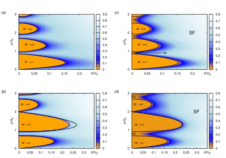
Figure 6: (Color online). Density fluctuations (left panels) and $\rho_{C}$ (right panels) for $U_{2}=\pm 0.1U_{0}$ and disorder in $U_{2}$ $\Delta/U_{0}=0.06$. MI lobes compared with the MF results (solid lines). Vanishing $\rho_{C}$ outside the MI lobes (solid lines), corresponds to the BG phase. Panels (a) and (c) correspond to the ferromagnetic case $U_{2}=-0.1U_{0}$ (a-c). The case $U_{2}=0.1U_{0}$ is reported in panels (b) and (d).

Figure 6 shows the effect of disorder for $U_{2}/U_{0}=\pm 0.1$ and $\Delta/U_{0}=0.06$. In the ferromagnetic case (plots (a) and (c)), disorder in $U_{2}$ has the same effect as the disorder in $\mu$. Similar to the scalar case, MI lobes are shrunk and BG phases appear between them. In contrast new features emerge in the antiferromagnetic case (plots (b) and (d)), where BG is formed only between lobes corresponding to $n$ and $n+1$ occupations with $n$-odd. No effect of disorder is visible between $n$ and $n+1$ MI lobes for $n$-even. A very simple explanation of that behavior may be obtained from Fig. 1. Note that for $U_{2}\in[0,U_{0}/2]$ the border separating $n$ and $n+1$ occupations for $n$-even in the $\mu-U_{2}$ plot is vertical (in $t=0$ limit). Thus changes (e.g. fluctuations) in $U_{2}$ do not modify the chemical potential at which the density changes. For $n$ odd in this range of $U_{2}$ the border is tilted, thus fluctuations in $U_{2}$ for a fixed $\mu$ change the density value which is favored for the ground state. Then, depending on the particular value of $U_{2}$ at a given site the density for the ground state changes. Interestingly, this picture, established for $t=0$, seems to hold also for finite $t$ as no BG is observed between the odd and even lobes. Further inspection of Fig. 1 reveals that in other possible ranges of $U_{2}$ the lines separating different densities are always tilted - indicating possibility of BG creation between the MI lobes. Incidentally, we can also interpret the same figure assuming fixed $U_{2}$ and fluctuating $\mu$ as the case discussed earlier in this paper. There are no horizontal lines in Fig.  1 thus all density borders are vulnerable to fluctuations in $\mu$. This is again consistent with the observation that for disorder in $\mu$ BG appears between all lobes.

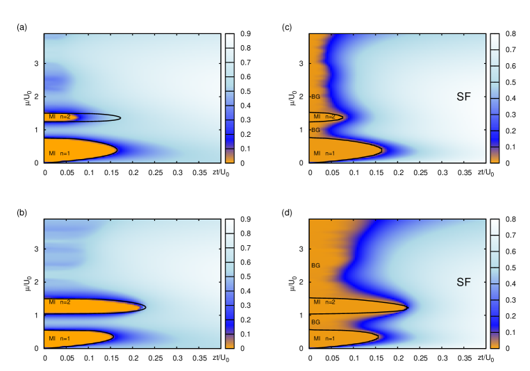
Figure 7: (Color online). Density fluctuations (left panels) and $\rho_{C}$ (right panels) for disorder in $U_{0}$ with $\Delta/U_{0}=0.25$ . MI lobes compared with the MF results (solid lines). Vanishing $\rho_{C}$ outside the MI lobes (solid lines), corresponds to the BG phase. Panels (a) and (c) correspond to $U_{2}/U_{0}=0.0$, (b) and (d) to $U_{2}/U_{0}=0.1$.

Finally, in Fig. 7 we show the result obtained for the disorder in $U_{0}$. As in the previous case we take $U_{0}^{i}=U_{0}+\epsilon_{i}$ with $\epsilon_{i}\in[-\Delta,\Delta]$. The plots report the case with zero and finite value of $U_{2}$ and $\Delta/U_{0}=0.25$. As explained in Gimperlein et al. (2005), in the $U_{2}=0$ case, lobes with occupation $n>(1+\Delta/U_{0})/(2\Delta/U_{0})$ disappear while the first one remains always stable. In our analysis we recover this behavior even for finite $U_{2}$. In both cases lobes separate and BG appears in between.

IV Summary-Open questions

We have analyzed the effects of disorder in the spin-1 BH model in which the spin interaction induces two different regimes, corresponding to a ferromagnetic and antiferromagnetic order, focusing mainly on the antiferromagnetic case, where the phase diagram differs more from the scalar case. We have considered here both, disorder introduced to the chemical potential (corresponding to an offset of energies at different sites) as well as disorder in the atom-atom interactions. As for the scalar bosons, we have observed the appearance of a compressible insulator - the BG phase - its character depending on the $U_{2}/U_{0}$ ratio. For small $U_{2}$ when Mott states with an odd number of atoms per site (also termed nematic since they have the mean value of all components of the spin equal zero, but a non vanishing singlet projection)exist in the absence of disorder, we expect the BG to be also nematic. For large $U_{2}$ however, when odd MI lobes do not exist already in the absence of disorder, we find a BG of singlets, a novel phase peculiar to bosons with spin.

Interestingly enough, in the presence of disorder on spinor coupling $U_{2}$, the system shows robustness against BG creation which does not emerge between $n$ and $n+1$ MI lobes for $n$- even. This is traced back to the insensitivity of the MI borders to changes in $U_{2}$ in the $\mu/U_{0}-U_{2}/U_{0}$ plane observed in the vanishing tunneling limit.

This work is only the first step towards understanding disorder on lattice spinorial bosons. For 1D systems density matrix renormalization group (DMRG) or its variants may be used to go beyond the mean field; work in this direction is in progress. For 2D, similar studies may be undertaken within QMC.

Finally, we remark the suitability of these systems for spin-glass studies. Notice that if one induces disorder in the $U_{2}$ coupling not preserving the ferromagnetic and anti-ferromagnetic character of the two-body interactions, i.e. if $\Delta>|U_{2}|$, a situation resembling frustration will appear in this model with antiferro and ferro sites randomly distributed along the lattice. Last but not least, a more realistic model of fluctuations in the interactions should be considered taking the details of optical Feshbach resonance into account.

References

- Ho (1998) T.-L. Ho, Phys. Rev. Lett. 81, 742 (1998).
- Ohmi and Machida (1998) T. Ohmi and K. Machida, J. Phys. Soc. Jpn. 67, 1822 (1998).
- Law et al. (1998) C. K. Law, H. Pu, and N. P. Bigelow, Phys. Rev. Lett. 81, 5257 (1998).
- Ho and Yip (2000) T.-L. Ho and S. K. Yip, Phys. Rev. Lett. 84, 4031 (2000).
- Fisher et al. (1989) M. P. A. Fisher, P. B. Weichman, G. Grinstein, and D. S. Fisher, Phys. Rev. B 40, 546 (1989).
- Imambekov et al. (2003) A. Imambekov, M. Lukin, and E. Demler, Phys. Rev. A 68, 063602 (2003).
- Tsuchiya et al. (2004) S. Tsuchiya, S. Kurihara, and T. Kimura, Phys. Rev. A 70, 043628 (2004).
- Rizzi et al. (2005) M. Rizzi, D. Rossini, G. De Chiara, S. Montangero, and R. Fazio, Phys. Rev. Lett. 95, 240404 (2005).
- Anderson (1958) P. W. Anderson, Phys. Rev. 109, 1492 (1958).
- Lewenstein et al. (2007) M. Lewenstein, A. Sanpera, V. Ahufinger, B. Damski, A. Sen, and U. Sen, Advances in Physics 56, 243 (2007).
- Horak et al. (1998) P. Horak, J.-Y. Courtois, and G. Grynberg, Phys. Rev. A 58, 3953 (1998).
- Boiron et al. (1999) D. Boiron, C. Mennerat-Robilliard, J. Fournier, L. Guidoni, C. Salomon, and G. Grynberg, Eur. Phys. J. D 7, 373 (1999).
- Roth and Burnett (2003) R. Roth and K. Burnett, Phys. Rev. A 68, 023604 (2003).
- Damski et al. (2003) B. Damski, J. Zakrzewski, L. Santos, P. Zoller, and M. Lewenstein, Phys. Rev. Lett. 91, 080403 (2003).
- Diener et al. (2001) R. B. Diener, G. A. Georgakis, J. Zhong, M. Raizen, and Q. Niu, Phys. Rev. A 64, 033416 (2001).
- Gavish and Castin (2005) U. Gavish and Y. Castin, Phys. Rev. Lett. 95, 020401 (2005).
- Massignan and Castin (2006) P. Massignan and Y. Castin, Phys. Rev. A 74, 013616 (2006).
- Gimperlein et al. (2005) H. Gimperlein, S. Wessel, J. Schmiedmayer, and L. Santos, Phys. Rev. Lett. 95, 170401 (2005).
- Chin et al. (2010) C. Chin, R. Grimm, P. Julienne, and E. Tiesinga, Rev. Mod. Phys. 82, 1225 (2010).
- Ma et al. (1986) M. Ma, B. I. Halperin, and P. A. Lee, Phys. Rev. B 34, 3136 (1986).
- Giamarchi and Schulz (1988) T. Giamarchi and H. J. Schulz, Phys. Rev. B 37, 325 (1988).
- Sanchez-Palencia and Lewenstein (2010) L. Sanchez-Palencia and M. Lewenstein, Nature Physics 6, 87 (2010).
- Ahufinger et al. (2005) V. Ahufinger, L. Sanchez-Palencia, A. Kantian, A. Sanpera, and M. Lewenstein, Phys. Rev. A 72, 063616 (2005).
- Sanpera et al. (2004) A. Sanpera, A. Kantian, L. Sanchez-Palencia, J. Zakrzewski, and M. Lewenstein, Phys. Rev. Lett. 93, 040401 (2004).
- Kimura et al. (2006) T. Kimura, S. Tsuchiya, M. Yamashita, and S. Kurihara, J. Phys. Soc. Jpn. 75, 074601 (2006).
- Jaksch et al. (1998) D. Jaksch, C. Bruder, J. I. Cirac, C. W. Gardiner, and P. Zoller, Phys. Rev. Lett. 81, 3108 (1998).
- Koashi and Ueda (2000) M. Koashi and M. Ueda, Phys. Rev. Lett. 84, 1066 (2000).
- Wu (1996) Y. Wu, Phys. Rev. A 54, 4534 (1996).
- Demler and Zhou (2002) E. Demler and F. Zhou, Phys. Rev. Lett. 88, 163001 (2002).
- Chen and Levy (1973) H. H. Chen and P. M. Levy, Phys. Rev. B 7, 4267 (1973).
- Papanicolaou (1988) N. Papanicolaou, Nuclear Physics B 305, 367 (1988).
- Delande and Zakrzewski (2009) D. Delande and J. Zakrzewski, Phys. Rev. Lett. 102, 085301 (2009).
- Greiner et al. (2002) M. Greiner, O. Mandel, T. Esslinger, T. W. Hänsch, and I. Bloch, Nature 415, 39 (2002).
- Kimura et al. (2005) T. Kimura, S. Tsuchiya, and S. Kurihara, Phys. Rev. Lett. 94, 110403 (2005).
- Batrouni et al. (2009) G. G. Batrouni, V. G. Rousseau, and R. T. Scalettar, Phys. Rev. Lett. 102, 140402 (2009).
- Bissbort and Hofstetter (2009) U. Bissbort and W. Hofstetter, Europhys. Lett. 86, 50007 (2009).
- Bissbort et al. (2010) U. Bissbort, R. Thomale, and W. Hofstetter, Phys. Rev. A 81, 063643 (2010).
- Damski and Zakrzewski (2006) B. Damski and J. Zakrzewski, Phys. Rev. A 74, 043609 (2006).
- Schneider et al. (2008) U. Schneider, L. Hackermüller, S. Will, T. Best, I. Bloch, T. A. Costi, R. W. Helmes, D. Rasch, and A. Rosch, Science 322, 1520 (2008).
- Pollet et al. (2009) L. Pollet, N. V. Prokof’ev, B. V. Svistunov, and M. Troyer, Phys. Rev. Lett. 103, 140402 (2009).
- Fallani et al. (2008) L. Fallani, C. Fort, and M. Inguscio, Adv. At. Mol. Opt. Phys. 56, 119 (2008).
- Fedichev et al. (1996) P. O. Fedichev, Y. Kagan, G. V. Shlyapnikov, and J. T. M. Walraven, Phys. Rev. Lett. 77, 2913 (1996).
- Bohn and Julienne (1997) J. L. Bohn and P. S. Julienne, Phys. Rev. A 56, 1486 (1997).
- Theis et al. (2004) M. Theis, G. Thalhammer, K. Winkler, M. Hellwig, G. Ruff, R. Grimm, and J. H. Denschlag, Phys. Rev. Lett. 93, 123001 (2004).
- Papoular et al. (2010) D. J. Papoular, G. V. Shlyapnikov, and J. Dalibard, Phys. Rev. A 81, 041603 (2010).