The Quasinormal Mode Spectrum of a Kerr Black Hole in the Eikonal Limit

Abstract

It is well established that the response of a black hole to a generic perturbation is characterized by a spectrum of damped resonances, called quasinormal modes; and that, in the limit of large angular momentum ($l\gg 1$), the quasinormal mode frequency spectrum is related to the properties of unstable null orbits. In this paper we develop an expansion method to explore the link. We obtain new closed-form approximations for the lightly-damped part of the spectrum in the large-$l$ regime. We confirm that, at leading order in $l$, the resonance frequency is linked to the orbital frequency, and the resonance damping to the Lyapunov exponent, of the relevant null orbit. We go somewhat further than previous studies to establish (i) a spin-dependent correction to the frequency at order $1/l$ for equatorial ($m=\pm l$) modes, and (ii) a new result for polar modes ($m=0$). We validate the approach by testing the closed-form approximations against frequencies obtained numerically with Leaver’s method.

I Introduction

Quasinormal modes (QNMs) are damped resonances which play a key role in black hole dynamics Kokkotas-Schmidt ; Nollert ; Ferrari-Gualtieri ; Berti-Cardoso-Starinets . For example, after the merger of a pair of black holes, the composite system ‘rings down’ through gravitational wave emission until it settles down into a quiescent axisymmetric Kerr phase. The gravitational wave signal from ringdown is dominated by the least-damped QNM resonances. Chandrasekhar Chandrasekhar was moved to compare the ringdown signal to the dying pure notes sounded by a bell. The analogy is apt; when a bell is struck, the dying tones depend only on the properties of the bell, rather than the hammer used to strike it, which affects only the relative degree of excitation of overtones. Likewise, the QNM spectrum depends only on the underlying properties of the black hole, rather than the complicated details of any initial perturbation.

Physically, a black hole quasinormal mode is a decaying resonance which satisfies a pair of causally-motivated boundary conditions (typically being ingoing at the event horizon, and outgoing at spatial infinity). Mathematically, ‘quasinormal ringing’ emerges from a sum of residues of poles of the Green function in the complex frequency domain Leaver-1986 . Each pole corresponds to a quasinormal mode of a single complex frequency. The real part of the frequency corresponds to the oscillation rate and the (negative) imaginary part corresponds to the damping rate.

In the Kerr spacetime QNMs are labelled by three indices: multipole $l$, azimuthal number $m$ and overtone number $n\geq 0$. The QNM spectrum depends only on the properties of the field (i.e. spin $s$) and the underlying black hole geometry (i.e. mass $M$, charge $Q$, angular momentum $J=aM$). In this paper, we concern ourselves with the most astrophysically-relevant case: the uncharged non-extremal Kerr black hole ($0\leq J<M^{2}$ and $Q=0$).

A wide range of methods have been developed for determining QNMs. A non-exhaustive list Berti includes (i) time domain methods Vishveshwara ; Dorband ; (ii) direct integration in the frequency domain Chandrasekhar-Detweiler ; (iii) inverse potential methods Blome-Mashhoon ; Ferrari-Mashhoon ; (iv) WKB methods Mashhoon-1983 ; Schutz-Will-1985 ; Iyer-Will ; Iyer ; Seidel-Iyer ; Kokkotas ; Konoplya ; (v) phase-integral methods Phase-integral1 ; Phase-integral2 ; Natario-Schiappa ; (vi) continued fraction method Leaver-1985 ; Nollert-1993 ; (vii) a semi-classical expansion method Dolan-Ottewill ; and (viii) an asymptotic iteration method Cho-Cornell-Doukas-Naylor-2009 ; Cho-Cornell-Doukas-Naylor-2010 . Review articles Kokkotas-Schmidt ; Nollert ; Ferrari-Gualtieri ; Berti-Cardoso-Starinets explore some of these methods in greater depth.

The quasinormal frequencies of the Kerr black hole were first computed by Detweiler Detweiler , and later by Leaver Leaver-1985 , Seidel and Iyer Seidel-Iyer , Kokkotas Kokkotas and Onozawa Onozawa (among others). In essence, the problem of accurately determining the QNMs of the Kerr black hole numerically has been ‘solved’ for a quarter of a century; the method introduced by Leaver Leaver-1985 is fast, reliable and accurate, and with certain modifications Nollert-1993 , robust at large overtones $n$ and angular momenta $l,m$. However, a numerical method provides little by way of physical insight. In contrast, approximation methods aim to provide some insight, perhaps at the expense of accuracy and applicability. For example, a body of work on the WKB method Mashhoon-1983 ; Schutz-Will-1985 ; Iyer-Will ; Iyer ; Seidel-Iyer ; Konoplya in spherically-symmetric spacetimes ‘explains’ the relationship between the low-overtone frequencies and the shape of the peak of the radial potential Iyer-Will . The low-overtone QNM spectrum of the Kerr black hole can be obtained via the WKB method Seidel-Iyer ; Kokkotas , although the expansion formulae are somewhat complicated.

It has been known for many years that quasinormal modes are intimately linked to the existence and properties of unstable photon orbits Goebel ; Ferrari-Mashhoon . A quarter-century ago, Mashhoon Mashhoon examined an aggregate of test null rays in orbit in the equatorial plane of a Kerr-Newman ($Q>0$) black hole near the co-rotating circular orbit. Mashhoon’s analysis suggested that, in the eikonal regime ($l\gg 1$), the maximally-corotating mode ($m=l$) has the frequency

$$\omega_{ln}^{m=l}\approx l\omega_{+}-i\lambda_{+}(n+1/2)$$ (1)

where $\omega_{+}$ is the Kepler frequency for null rays on the unstable orbit and $\lambda_{+}$ is the decay rate of the unstable orbit (subsequently identified as the Lyapunov exponent Lyapunov1 ; Lyapunov2 ; Lyapunov3 ). These orbital quantities were plotted as a function of $a$ in Ferrari-Mashhoon-letter ; see also our Fig. 2. The ‘geometric-optics’ approach of Mashhoon is both appealing and insightful. For example, it neatly ‘explains’ why the maximally corotating modes ($m=l$) are faster-oscillation and slower-decaying than the other modes ($m<l$). However, Mashoon’s original analysis was only ‘indirect’, in the sense that the Teukolsky equation, which describes massless perturbations of the Kerr spacetime, was not solved directly. So, for instance, it is not clear from (1) what effect the spin of the perturbing field has on the frequency spectrum.

A recent work by Hod Hod demonstrated that a bridge may be built between “geometric-optics” intuition and “Teukolsky equation” exactitude. By analysizing the Teukolsky equation in the extremal limit ($a\rightarrow M$), Hod showed that (1) is indeed good approximation.

The aim of this paper to show that improved approximations to QNM frequencies may be obtained by directly analysing the Teukolsky equation, without recourse to WKB methods. We go further than other studies (such as Mashhoon Mashhoon and Hod Hod ) to obtain frequency expansions in closed form which include the leading-order effect of the spin of the perturbing field, and which are valid outside the extremal regime (i.e. for all $a$). As well as considering the equatorial modes ($m=\pm l$) we also analyse the ‘polar’ ($m=0$) modes (see Fig. 1 for illustration). We confirm that the expansions provide the correct fits to the numerically-determined spectrum, in the limit $l\gg 1$.

To obtain our new analytic results, we apply a recently-introduced expansion method Dolan-Ottewill . Previously, this method has been applied to a range of spherically-symmetric spacetimes Dolan-Ottewill , and to a simple cylindrically-symmetric system (the ‘draining vortex’) Leandro . In this paper, we extend the method to treat an axisymmetric system for the first time. The key idea behind our approach is that the properties of modes of high angular momentum $l\gg 1$ are related to the properties of the unstable photon orbits of the spacetime (see Fig. 1 and Teo ). This idea is not new Goebel ; the novel ingredient is a ‘semi-classical’ ansatz enables us build a bridge between the classical ‘geodesic’ picture of a battery of null geodesics near the photon orbit Mashhoon , and a perturbative analysis at the level of the Teukolsky equation. This ansatz allows the QNM frequencies and wavefunction to be expanded in inverse powers of $l$.

The remainder of this paper is organized as follows: in Sec. II we describe the Kerr spacetime, null geodesics, and the Teukolsky equation; in Sec. III we develop the expansion method and obtain the key analytic results; in Sec. IV we validate the approach by testing the expansion against numerical results. We conclude in Sec. V with a brief discussion.

II Spacetime, Geodesics and Waves

In this section we lay some groundwork, and give geometrical motivation for the QNM analysis which follows in later sections. In Sec. II.1 we review some properties of the Kerr spacetime; in Sec. II.2 we consider the null geodesics of the spacetime, and the unstable photon orbits Teo ; and in Sec. II.3 we recap the theory of weak-field perturbations of Kerr.

II.1 The Kerr Spacetime

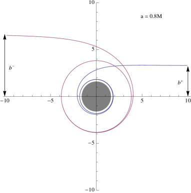
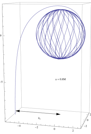
Figure 1: Critical null geodesics for $a=0.8M$. These plots show the special null geodesics which impinge from infinity and asymptote to the unstable photon orbits. The 2D plot (left) shows co- and counter-rotating orbits in the equatorial plane (with the spin axis pointing out of the page). The 3D plot (right) shows a polar orbit, with the spin axis of the BH pointing up the page.

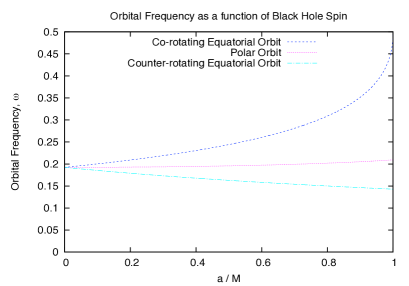
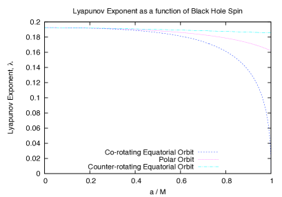
Figure 2: Parameters for Unstable Photon Orbits around a Kerr black hole as a function of $a=J/M$. The left plot shows the orbital frequency with respect to coordinate time $t$ (time measured at spatial infinity). The right plot shows the Lyapunov exponent, which controls the decay rate of QNMs. The lines are for the special cases of prograde and retrograde equatorial orbits (see also Fig. 1 & 2 in Ferrari-Mashhoon-letter ) and the polar orbit, discussed in Sec. II.2. General orbits would correspond to lines between these limits.

The Kerr metric Kerr-1963 describes the spacetime around a rotating uncharged black hole in vacuum (for details see e.g. Chandrasekhar ; MTW ; WiltshireVisserScott ). In the Boyer-Lindquist coordinate system $\{t,r,\theta,\phi\}$ the line element takes the form

$$ds^{2}=-(1-2Mr/\rho^{2})dt^{2}-(4aMr\sin^{2}\theta/\rho^{2})dtd\phi+(\rho^{2}/\Delta)dr^{2}+\rho^{2}d\theta^{2}+\sin^{2}\theta(r^{2}+a^{2}+2Ma^{2}r\sin^{2}\theta/\rho^{2})d\phi^{2},$$ (2)

where $\Delta\equiv r^{2}-2Mr+a^{2}$ and $\rho^{2}\equiv r^{2}+a^{2}\cos^{2}\theta$, and where $M$ and $aM$ are the mass and angular momentum of the black hole. The spacetime has an ergosphere within $r<2M$ and horizons at $r=r_{h\pm}\equiv M\pm\sqrt{M^{2}-a^{2}}$.

II.2 Null Geodesics and Orbits

Killing vector fields (satisfying $\xi_{(a;b)}=0$) associated with time translation $\xi^{a}_{(t)}$ and rotation around the symmetry axis $\xi^{a}_{(\phi)}$ give rise to two constants of motion along a geodesic with tangent vector $u^{a}$: an ‘energy’ $E\equiv-\xi^{a}_{(t)}u_{a}$ and an ‘azimuthal angular momentum’ $L_{z}\equiv\xi^{a}_{(\phi)}u_{a}$. The existence of a Killing tensor $K_{ab}$ satisfying $K_{(ab;c)}=0$ implies a further constant of motion, the ‘Carter constant’ Carter-1968 defined as $\mathcal{Q}=K_{ab}u^{a}u^{b}+L_{z}^{2}-E^{2}$. The Carter constant governs the motion of geodesics in the latitudinal direction. The equations of motion for null rays can be written in first order form Chandrasekhar ; Teo ; MTW ; Drasco-Hughes-2004 as

$$\rho^{2}\dot{t} = \left(\Sigma^{2}E-2MarL_{z}\right)/\Delta,$$ (3)

$$\rho^{2}\dot{\phi} = \left(2MarE+(\rho^{2}-2Mr)\frac{L_{z}}{\sin^{2}\theta}\right)/\Delta$$ (4)

$$\left(\rho^{2}\dot{r}\right)^{2} = E^{2}r^{4}+(a^{2}E^{2}-L_{z}^{2}-\mathcal{Q})r^{2}+2M\left[(aE-L_{z})^{2}+\mathcal{Q}\right]r-a^{2}\mathcal{Q},$$ (5)

$$\left(\rho^{2}\dot{\theta}\right)^{2} = \mathcal{Q}-\left[\frac{L_{z}^{2}}{\sin^{2}\theta}-a^{2}E^{2}\right]\cos^{2}\theta,$$ (6)

where $\Sigma^{2}=(r^{2}+a^{2})^{2}-a^{2}\Delta\sin^{2}\theta$ and an overdot denotes differentiation with respect to an affine parameter. Note that the $r$ and $\theta$ equations may be decoupled into ordinary differential equations by using the ‘Mino time’ Mino ; Drasco-Hughes-2004 parameter $\nu$ defined by $d\nu=d\lambda/\rho^{2}$. For our purposes this is not necessary.

In the following section we consider three sets of constant-$r$ null orbits: prograde and retrograde equatorial orbits with $\mathcal{Q}=0$ and polar orbits with $L_{z}=0$. These orbits are illustrated in Fig. 1. The cases are henceforth distinguished using subscripts $+$, $-$ and $\circ$, respectively; for example, we will denote the orbital radii by $\hat{r}_{+}$, $\hat{r}_{-}$ and $\hat{r}_{\circ}$ and the angular frequencies (with respect to coordinate time $t$) by $\omega_{+}$, $\omega_{-}$ and $\omega_{\circ}$. Figure 2 shows the orbital frequency and Lyapunov exponent for these special orbits as a function of black hole rotation $a$.

II.2.1 Equatorial orbits

Consider first null geodesics in the equatorial plane, with $\mathcal{Q}=0$. The ratio of azimuthal angular momentum to energy defines an impact parameter (see Fig. 1),

$$b=L_{z}/E.$$ (7)

Null geodesics in the equatorial plane are governed by the orbital equation

$$\dot{r}^{2}=\frac{L_{z}^{2}}{b^{2}}\left[1+\frac{a^{2}-b^{2}}{r^{2}}+\frac{2M(b-a)^{2}}{r^{3}}\right]$$ (8)

Perpetual photon orbits are possible if conditions $\dot{r}=0$ and $\ddot{r}=0$ can be satisfied simultaneously. It is straightforward to show that both prograde $(+)$ and retrograde $(-)$ orbits exist, at orbital radii $\hat{r}_{\pm}$,

$$\hat{r}_{\pm}=2M\left[1+\cos\left(\tfrac{2}{3}\cos^{-1}(\mp a/M)\right)\right],$$ (9)

with critical impact parameters $b_{\pm}$ given by

$$b_{\pm}=\pm 3\sqrt{M\hat{r}_{\pm}}-a.$$ (10)

Note that we define the critical impact parameter $b$ so that it is negative for the retrograde trajectory. The orbital frequency $\omega_{\pm}=\dot{\phi}/\dot{t}$ of the circular orbit is obtained from the ratio of the $\phi$ and $t$ equations (3 and 4), and it is straightforward to show that it is simply

$$\omega_{\pm}=\frac{1}{\left|b_{\pm}\right|}=\frac{M^{1/2}}{(\hat{r}_{\pm})^{3/2}\pm aM^{1/2}}.$$ (11)

In the critical case, the orbital equation (8) can be factorized into

$$\dot{r}^{2}=\frac{L_{z}^{2}}{b_{\pm}^{2}}\left(1-\frac{\hat{r}_{\pm}}{r}\right)^{2}\left(1+\frac{2\hat{r}_{\pm}}{r}\right).$$ (12)

In Mashhoon ; Lyapunov1 ; Hod it was established that the decay rate for the equatorial circular orbits is controlled by Lyapunov exponent $\lambda$ (see Eq. (1)). For the equatorial orbits Lyapunov1 , it has been shown that the Lypanov exponent is

$$\lambda_{\pm}=\frac{1-2x_{\pm}}{\left|b_{\pm}\right|\sqrt{1-x_{\pm}^{2}}}$$ (13)

where $x_{\pm}$ is the ratio

$$x_{\pm}\equiv a/b_{\pm}$$ (14)

Note that $b_{-}<0$ and hence $x_{-}<0$.

In the Schwarzschild limit ($a\rightarrow 0$) we recover $\hat{r}_{\pm}=3M$, $b_{\pm}=\sqrt{27}\,M$ and $\omega_{\pm}=\lambda_{\pm}=1/(\sqrt{27}M)$. In the extremal limit ($a\rightarrow M$) we have $\hat{r}_{-}=4M$, $b_{-}=-7M\Rightarrow\omega_{-}=1/(7M)$, $\lambda_{-}=3/(7\sqrt{5}M)$ and $\hat{r}_{+}=M$, $b_{+}=2M\Rightarrow\omega_{+}=1/(2M)$ and $\lambda_{+}=0$. Note that the decay rate of the co-rotating mode tends to zero in the extremal limit (as many authors have previously observed).

II.2.2 Polar orbits

Consider next the special case of trajectories with zero azimuthal angular momentum ($L_{z}=0$), which we will refer to as ‘polar’ geodesics. For polar geodesics we may define the natural impact parameter

$$b^{2}=\mathcal{Q}/E^{2}+a^{2}$$ (15)

which corresponds to the perpendicular distance between the geodesic and the rotation axis (measured at spatial infinity). Note that polar geodesics are parallel to the rotation axis at spatial infinity, as shown in Fig. 1.

Null polar geodesics are governed by the equation

$$\left(E^{-1}\rho^{2}\dot{r}\right)^{2}\equiv R(r)=r^{4}+(2a^{2}-b^{2})r^{2}+2Mb^{2}r+a^{2}(a^{2}-b^{2})$$ (16)

An unstable orbit arises at radius $r=\hat{r}_{\circ}$ where $R(\hat{r}_{\circ})=0$ and $R^{\prime}(\hat{r}_{\circ})=0$, given by

$$\hat{r}_{\circ}=M+2\sqrt{M^{2}-a^{2}/3}\,\cos\left[\frac{1}{3}\cos^{-1}\left(\frac{M(M^{2}-a^{2})}{(M^{2}-a^{2}/3)^{3/2}}\right)\right]$$ (17)

(see e.g. Eq. (14) in Teo ). The critical impact parameter is given by

$${b}_{\circ}^{2}=\frac{(3\hat{r}_{\circ}^{2}-a^{2})(\hat{r}_{\circ}^{2}+a^{2})}{\hat{r}_{\circ}^{2}-a^{2}},$$ (18)

and in the critical case $b=b_{\circ}$, the radial equation (16) can be factorized into

$$R(r)=\left(r-\hat{r}_{\circ}\right)^{2}\left(r^{2}+2\hat{r}_{\circ}r-a^{2}({b}_{\circ}^{2}-a^{2})/\hat{r}_{\circ}^{2}\right).$$ (19)

The period $T_{\circ}$ for a null geodesic on the unstable polar orbit at $r=\hat{r}_{\circ}$ can be found from integrating the ratio of the $t$ and $z=\cos(\theta)$ equations (see Appendix A for details),

$$T_{\circ}=2\int_{-1}^{+1}\frac{dt}{dz}dz=2{d}_{\circ}\int_{-1}^{+1}\left(\frac{1+a^{2}z^{2}/{d}_{\circ}^{2}}{1-z^{2}}\right)^{1/2}dz=4{d}_{\circ}\,\text{ellipE}(ia/{d}_{\circ}).$$ (20)

where we have defined ${d}_{\circ}=\sqrt{{b}_{\circ}^{2}-a^{2}}\equiv\sqrt{Q}/E$, and $\text{ellipE}(\cdot)$ is the complete elliptic integral of the second kind Abramowitz-Stegun (a note of caution: $\text{ellipE}(k)$ is implemented in Maple as $\text{EllipticE}(k)$, but in Mathematica as $\text{EllipticE}(k^{2})$). Hence the orbital frequency is

$$\omega_{\circ}=\frac{\pi}{2{d}_{\circ}\,\text{ellipE}(ia/{d}_{\circ})}.$$ (21)

We expect the imaginary part of the QNM of the polar modes ($L_{z}=0$) to be related to the Lyapunov exponent $\lambda$ for the polar null orbits. In Appendix A it is shown to be

$$\lambda_{\circ}=\frac{\hat{r}_{\circ}}{({d}_{\circ})^{2}}\frac{\text{ellipK}\left(x_{\circ}/\sqrt{1+x_{\circ}^{2}}\right)}{\sqrt{1+x_{\circ}^{2}}\,\text{ellipE}(ix_{\circ})}\left(3-\frac{a^{2}{d}_{\circ}^{2}}{\hat{r}_{\circ}^{4}}\right)^{1/2},$$ (22)

where $\text{ellipK}(\cdot)$ is the complete elliptic integral of the first kind and we have defined the ratio

$$x_{\circ}=a/{d}_{\circ}.$$ (23)

In the extremal limit, $a\rightarrow M$, we have $\hat{r}_{\circ}/M=1+\sqrt{2}\approx 2.4142$ and $b_{\circ}/M\approx 4.8284$ and $M\omega_{\circ}\approx 0.20937$ and $M\lambda\approx 0.162006$. Unlike the corotating modes, the $m=0$ modes are still significantly damped in this limit (as is shown in Fig. 2).

II.2.3 General orbits

Above we considered two limiting cases: equatorial orbits restricted to $\theta=\pi/2$, and polar orbits that explore the full range of polar angles, $0\leq\theta\leq\pi$. A general orbit will explore a more limited range of polar angles, $\pi/2-\Delta\theta\leq\theta\leq\pi/2+\Delta\theta$. The angular range $\Delta\theta$ is a function of the ratio $L_{z}/\sqrt{\mathcal{Q}}$, with limiting cases $\Delta\theta(L_{z}/\sqrt{\mathcal{Q}}\rightarrow\infty)=0$ and $\Delta\theta(L_{z}/\sqrt{\mathcal{Q}}\rightarrow 0)=\pi/2$. It was shown in e.g. Teo that perpetual orbits exist for all ratios $L_{z}/\sqrt{\mathcal{Q}}$. A general analysis is left for future work.

II.3 Perturbations of the Kerr Spacetime

To analyse gravitational dynamics around a rotating black hole, one may examine perturbations of the metric tensor via Einstein’s equations linearized around the Kerr background (assuming the perturbations are “small”). This approach yields a set of coupled partial differential equations, which are difficult to analyze. An alternative approach is to consider perturbations of the Weyl and Ricci scalars using the Newman-Penrose formalism. This was the approach taken by Teukolsky Teukolsky-1972 ; Teukolsky-1973 , who decoupled and separated the equations to reduce them to a single ‘master equation’ for the radial part of the perturbation.

A ‘master equation’ describes massless perturbations of scalar ($|s|=0$), spinor ($|s|=1/2$), electromagnetic ($|s|=1$) and gravitational ($|s|=2$) types. In vacuum, the radial equation is

$$\Delta^{-s}\frac{d}{dr}\left(\Delta^{s+1}\frac{dR}{dr}\right)+\left(\frac{K^{2}-2is(r-M)K}{\Delta}+4is\omega r-\Lambda\right)R=0$$ (24)

(Eq. (4.8) in Teukolsky-1973 ) where $K\equiv(r^{2}+a^{2})\omega-am$. The angular separation constant $\Lambda=A_{lm}-2ma\omega+a^{2}\omega^{2}$ is determined from imposing physical boundary conditions at the poles ($\theta=0,\pi$) on the angular equation

$$\frac{d}{dz}\left[(1-z^{2})\frac{dS}{dz}\right]+\left[a^{2}\omega^{2}z^{2}-2am\omega sz+s+A_{lm}-\frac{(m+sz)^{2}}{1-z^{2}}\right]S=0,\quad\text{where}\;z=\cos\theta,$$ (25)

whose solutions are oblate spin-weighted spheroidal harmonics $S={}_{s}S_{lm}(a\omega;z)$ Abramowitz-Stegun . An expansion of the angular eigenvalue in powers of $a\omega$ is given in Seidel-1989 ; Berti-Cardoso-Casals .

Let us make the substitution $R(r)=r^{-1}\Delta^{-s}u(r)$ to write the radial equation (24) as

$$\frac{d^{2}u}{dr_{\ast}^{2}}-\frac{2s(r-M)}{r^{2}}\frac{du}{dr_{\ast}}+\left[\Omega^{2}-\frac{2is(r-M)\Omega}{r^{2}}-f\left(\frac{\Lambda}{r^{2}}+\frac{f^{\prime}}{r}+\frac{2Ms}{r^{3}}-\frac{4i\omega s}{r}\right)\right]u=0$$ (26)

where

$$f(r)=\Delta/r^{2}=1-2M/r+a^{2}/r^{2}$$ (27)

and

$$\Omega(r)=K(r)/r^{2}=(1+a^{2}/r^{2})\omega-am/r^{2}.$$ (28)

Here we have defined a tortoise coordinate $r_{\ast}$ via

$$\frac{dr_{\ast}}{dr}=f^{-1}.$$ (29)

Note that this definition differs from, e.g., Teukolsky Teukolsky-1973 , who defines instead $\tfrac{dr_{\ast}}{dr}=(r^{2}+a^{2})/\Delta$.

Quasinormal modes are the complex-frequency modes that are purely ingoing at the (outer) horizon ($r=r_{h+}$), and purely outgoing at spatial infinity, satisfying boundary conditions

$$u(r)\sim\left\{\begin{array}[]{ll}\exp(-i[\omega-am/r_{h+}^{2}]r_{\ast}),&r_{\ast}\rightarrow-\infty,\\ \exp(+i\omega r_{\ast}),&r_{\ast}\rightarrow+\infty.\end{array}\right.$$ (30)

III QNM Expansion Method

In this section we extend and develop the QNM expansion method first described in Dolan-Ottewill . The method has three steps: (i) introduce an ansatz for the wavefunction, inspired by the null geodesics near the perpetual orbit, (ii) expand the wavefunction and frequency in inverse powers of $m$ (or $l$), (iii) impose a continuity condition at the perpetual orbit radius (i.e. $r=\hat{r}_{\pm}$ or $r=\hat{r}_{\circ}$) to recover the expansion coefficients.

III.1 Equatorial modes of scalar field

Let us illustrate the method by considering first the maximally corotating modes, $m=l$, of the scalar wave equation ($s=0$). We seek solutions to (26) that satisfy the QNM boundary conditions (30). Step (i) is to propose an ansatz of the form

$$u(r)=\exp\left(i\int\beta(r)dr_{\ast}\right)v(r).$$ (31)

We demand that $\beta(r)$ has three properties. First, $\beta(r)$ should have a root at the circular orbit $r=\hat{r}_{+}$, so that $\beta$ changes sign here, and the solution passes smoothly from outgoing behaviour at infinity to ingoing behaviour at the horizon. Second, $\beta^{2}$ should be such that, upon insertion into Eq. (26), the resulting equation has an overall factor of $f$. That is,

$$-\beta^{2}+\Omega^{2}\propto f,$$ (32)

Third, $\beta$ should ensure that the QNM boundary conditions are satisfied, provided $v$ is regular at both horizon and infinity.

The third property suggests that $\beta$ has an overall factor of $\Omega(r)$ (defined in Eq. (28)), and the first property suggests that we take inspiration from the factorized form of the orbital equation (12) to write

$$\beta(r)=\Omega(r)\left(1-\frac{a(b-a)}{r^{2}}\right)^{-1}\left(1-\frac{\hat{r}_{+}}{r}\right)\left(1+\frac{2\hat{r}_{+}}{r}\right)^{1/2}$$ (33)

where $b=b_{+}$, defined in (10). It is straightforward to confirm that the second property (32) is satisfied,

$$-\beta^{2}+\Omega^{2}=f(r)\,\Omega^{2}\frac{(b-a)^{2}}{r^{2}}\left[1-\frac{a(b-a)}{r^{2}}\right]^{2}.$$ (34)

and that the QNM boundary conditions are satisfied if $v(r)$ is regular at the horizon and infinity. Upon substitution of the ansatz (31) into (26), and after dividing through by $f$, we reach the new radial equation

$$\frac{d}{dr}\left(f\frac{dv}{dr}\right)+2i\beta\frac{dv}{dr}+\left[\Omega^{2}\frac{(b-a)^{2}}{r^{2}}\left(1-\frac{a(b-a)}{r^{2}}\right)^{-2}+i\beta^{\prime}-\frac{\Lambda}{r^{2}}-\frac{f^{\prime}}{r}\right]v=0.$$ (35)

Step (ii) is to expand the wavefunction, frequency and angular eigenvalue in inverse powers of $m=l$, in the following manner,

$$b\,\omega = \varpi_{-1}m+\varpi_{0}+\varpi_{1}m^{-1}+\ldots$$ (36)

$$v(r) = \exp\left(S_{0}(r)+m^{-1}S_{1}(r)+\ldots\right)$$ (37)

$$\Lambda = \Lambda_{-2}m^{2}+\Lambda_{-1}m+\Lambda_{0}+\ldots$$ (38)

Here, $\{\varpi_{-1},\varpi_{0},\ldots\}$ and $\{\Lambda_{-2},\Lambda_{-1},\ldots\}$ are coefficients to be determined, and $\{S_{0}(r),S_{1}(r),\ldots\}$ are regular functions of $r$. Inserting (36, 37, 38) into (26) and grouping together like powers of $m$ leads to a system of equations,

$$\mathcal{O}(m^{2})\,:\; \frac{(b-a)^{2}}{b^{2}}\left[\left(1+\frac{a^{2}}{r^{2}}\right)\varpi_{-1}-\frac{ab}{r^{2}}\right]^{2}\left(1-\frac{a(b-a)}{r^{2}}\right)^{-2}-\Lambda_{-2}=0$$ (39)

$$\mathcal{O}(m^{1})\,:\; 2i\beta_{0}\frac{dS_{0}}{dr}+i\beta_{0}^{\prime}-\frac{\Lambda_{-1}}{r^{2}}+2\left(1+\frac{a^{2}}{r^{2}}\right)\varpi_{0}\frac{(b-a)^{2}}{b^{2}r^{2}}=0$$ (40)

$$\mathcal{O}(m^{0})\,:\; \ldots$$ (41)

Here $\beta_{0}(r)=(\varpi_{-1}/b)(1-a(b-a)/r^{2})^{-1}(1-\hat{r}_{+}/r)(1+2\hat{r}_{+}/r)^{1/2}$ and $b=b_{+}$ given in Eq. (10). A major difference with the Schwarzschild case is that the angular expansion coefficients $\Lambda_{k}$ is also dependent on frequency, through $a\omega$. This challenge is not insurmountable. First we note that $\Lambda_{-2}=(1-a\varpi_{-1}/b)^{2}$. It is trivial to then show that the choice $\varpi_{-1}=1$ satisfies Eq. (39). To find higher-order coefficients, we may use the series expansion of the eigenvalue given in Seidel-1989 ; Berti-Cardoso-Casals . We find

$$\Lambda_{-2} = (1-x)^{2}$$ (42)

$$\Lambda_{-1} = \mathcal{S}_{1}-2x(1-x)\varpi_{0}$$ (43)

$$\Lambda_{0} = -2s^{2}x\mathcal{S}_{2}+\frac{3x^{2}}{4}\mathcal{S}_{3}+x\frac{d\mathcal{S}_{1}}{dx}\varpi_{0}$$ (44)

where $x=a/b$ and

$$\mathcal{S}_{1}=1-\tfrac{1}{2}x^{2}-\tfrac{1}{8}x^{4}-\tfrac{1}{16}x^{6}+\mathcal{O}(x^{8}) \doteq \left(1-x^{2}\right)^{1/2}$$ (45)

$$\mathcal{S}_{2}=1+x+x^{2}+x^{3}+x^{4}+x^{5}+\mathcal{O}(x^{6}) \doteq (1-x)^{-1}$$ (46)

$$\mathcal{S}_{3}=1+x^{2}+x^{4}+\mathcal{O}(x^{6}) \doteq (1-x^{2})^{-1}$$ (47)

Though Seidel Seidel-1989 provides an expansion to sixth order in $a\omega$, this provides only the first few terms of a (presumably) infinite series. Above, we used intuition to ‘guess’ a closed form from the first few terms of the series expansion (the results to the right of the $\doteq$ symbol). Mathematica can be used to obtain further terms in the expansion of the spheroidal eigenvalue in the scalar case ($s=0$); the higher terms are consistent with the assumption. In Sec. IV we test the resulting frequencies against numerical results and find the expected agreement.

Next we demand that the radial function $S_{0}(r)$, which features in the expansion of the wavefunction (37), is continuous at $r=\hat{r}_{+}$ (where $\beta(\hat{r}_{+})=0$). After inserting result (43) into (40) and evaluating at $r=\hat{r}_{+}$ and rearranging, we obtain the coefficient

$$\varpi_{0}=\frac{1-2x}{2\sqrt{1-x^{2}}}(1-i)$$ (48)

The function $S_{0}$ may then be determined by substituting (48) back into (40) and rearranging to find $S_{0}^{\prime}$, then integrating.

In principle, we may continue in this fashion to determine the higher-order coefficients $\varpi_{1},\varpi_{2},\ldots$ and phase functions $S_{1}(r),S_{2}(r),\ldots$, with the help of a symbolic algebra package. In practice it is a challenge to continue the expansion beyond $\mathcal{O}(m^{-2})$, due to the frequency dependence of the angular eigenvalue. Results to this order are given in Eq. (51).

To look for higher modes ($n>0$) one must first modify the ansatz for the wavefunction (37), as shown in Dolan-Ottewill . This technique follows through to the axisymmetric case without additional difficulties, although the calculation is not pursued here.

III.2 Equatorial modes of higher spin

Let us now show how one may generalise the previous analysis to treat fields of higher spin ($s\neq 0$). As in Sec. III.1, we start with Eq. (26) and once again propose an ansatz of the form (31). As in Sec. III.1, we demand that $\beta$ obeys three conditions, but now the second condition (32) becomes

$$-\left(\beta+\frac{is(r-M)}{r^{2}}\right)^{2}+\left(\Omega-\frac{is(r-M)}{r^{2}}\right)^{2}\propto f,$$ (49)

The conclusion is that

$$\beta+\frac{is(r-M)}{r^{2}}=\left(\Omega-\frac{is(r-M)}{r^{2}}\right)\left(1-\frac{a(b-a)}{r^{2}}\right)^{-1}\left(1-\frac{\hat{r}_{+}}{r}\right)\left(1+\frac{2\hat{r}_{+}}{r}\right)^{1/2}.$$ (50)

It is straightforward to verify that $\beta$ satisfies the QNM boundary conditions at the horizon and at infinity.

The method proceeds through step (ii) and (iii) as in the scalar case. The method was automated using a symbolic algebra package. We now present the key results for the equatorial modes.

III.3 Equatorial Modes: Key Results

Applying the method described above, we find that the fundamental ($n=0$) maximally co-rotating ($m=l$) frequency $\omega^{(m=l)}_{n=0}$ has the following ‘eikonal’ expansion :

$$b_{+}\,\omega^{(m=l)}_{l,n=0}=m+\frac{(1-2x)}{2\sqrt{1-x^{2}}}(1-i)+\frac{(1-2x)}{216m(1-x^{2})^{2}}\left[(7+44x+127x^{2})-72s^{2}(1+x)^{2}\right]+\mathcal{O}(m^{-2})$$ (51)

where here $x=x_{+}\equiv a/b_{+}$ and the critical impact parameter $b_{+}$ was defined in (10). We established in Eq. (11) that $1/b_{+}$ is equal to the Kepler orbital frequency $\omega_{+}$ for null rays in corotating circular orbit. Furthermore, the leading-order imaginary component is equal to one-half of the Lyapunov exponent given in (13) (and Refs. Mashhoon ; Lyapunov1 ).

To leading order, our result is consistent with the outcome of the geodesic analysis of Mashhoon Mashhoon , Cardoso et al. Lyapunov1 and Hod (Hod , Eq. 3 and 4), and with the wave-equation analysis of Hod in the extremal regime. Note however that result (51) goes two steps further. Firstly, it includes a spin-independent correction to the real part of frequency at order $\mathcal{O}(m^{0})$, which has not been previously obtained. Secondly, it also includes the spin-dependent correction at order $\mathcal{O}(m^{-1})$ for the first time. In Sec. IV we compare result (51) against numerically-determined frequencies, to verify that both new terms are correct.

The expansion of the fundamental ($n=0$) maximally counter-rotating ($m=-l$) frequency $\omega_{n=0}^{(m=-l)}$ is

$$b_{-}\,\omega^{(m=-l)}_{l,n=0}=m-\frac{(1-2x)}{2\sqrt{1-x^{2}}}(1-i)+\frac{(1-2x)}{216m(1-x^{2})^{2}}\left[(7+44x+127x^{2})-72s^{2}(1+x)^{2}\right]+O(m^{-2})$$ (52)

where here $x=x_{-}\equiv a/b_{-}$. Note that the counter-rotating impact parameter $b_{-}$ given by (10) is negative, as is $x$ (for positive $a$). Result (52) may be obtained from result (51) via the simultaneous replacements $b_{+}\rightarrow b_{-}$, $x_{+}\rightarrow x_{-}$, $m\rightarrow-m$ and $\omega_{n=0}^{(m=l)}\rightarrow-\omega_{n=0}^{(m=-l)}$.

The QNM spectrum has the following symmetry property:

$$\omega_{lmn}=-\omega_{l,-m,n}^{\ast}.$$ (53)

Therefore frequencies with negative real part may be obtained by applying (53) to Eqs. (52) and (51).

III.4 QNMs of polar modes ($m=0$)

In Sec. II.2.2 we considered ‘polar’ geodesics, which have zero azimuthal angular momentum $L_{z}=0$ and pass through the north and south poles $\theta=0,\pi$. Here we apply the expansion method to the Teukolsky equation to find the corresponding $m=0$ QNM frequencies.

For brevity, let us consider scalar waves ($s=0$) here, as it turns out that the leading order terms (at $l^{1}$ and $l^{0}$) are not spin-dependent. The appropriate ansatz for the polar modes is again of the form (31), with condition (ii) (Eq. (32)) suggesting the choice

$$\beta^{2}=\Omega^{2}-f(r)\frac{\omega^{2}b_{\circ}^{2}}{r^{2}}=\frac{\omega^{2}R(r)}{r^{4}},$$ (54)

where $b_{\circ}$ is the critical impact parameter (18) and $R(r)$ is the quartic defined in Eq. (16), with factorization given by Eq. (19).

Inserting the ansatz (54) into (26) leads to

$$\left(fv^{\prime}\right)^{\prime}+2i\beta(r)v^{\prime}+\left[i\beta^{\prime}+\frac{\omega^{2}b_{c}^{2}-\Lambda}{r^{2}}-\frac{f^{\prime}}{r^{2}}\right]v=0.$$ (55)

Next we expand in inverse powers of $L=l+1/2$,

$$b_{\circ}\omega = \varpi_{-1}L+\varpi_{0}+\varpi_{1}L^{-1}+\ldots$$ (56)

$$v(r) = \exp\left(S_{0}(r)+S_{1}(r)L^{-1}+\ldots\right)$$ (57)

$$\Lambda = \Lambda_{-2}L^{2}+\Lambda_{-1}L+\Lambda_{0}+\ldots$$ (58)

Now group terms in (55) order-by-order in $L$,

$$\frac{\varpi_{-1}^{2}-\Lambda_{-2}}{r^{2}} = 0$$ (59)

$$\frac{2i\varpi_{-1}\left(r^{2}+2r\hat{r}_{\circ}-a^{2}d^{2}/\hat{r}_{\circ}^{2}\right)}{r^{2}}(r-\hat{r}_{\circ})S^{\prime}_{0}(r)+\frac{2\varpi_{-1}\varpi_{0}}{r^{2}}+i\beta_{0}^{\prime}-\frac{\Lambda_{-1}}{r^{2}} = 0$$ (60)

$$\ldots = 0$$ (61)

Once again, there remains an obstacle to progress: the frequency-dependence of the angular eigenvalue $\Lambda$. The angular eigenvalue of the scalar field ($s=0$) for the polar mode $\Lambda_{l,m=0}$ has the following expansion:

$$\Lambda_{l,m=0}=L^{2}+\left(\frac{c^{2}}{2}-\frac{1}{4}\right)+\frac{c^{4}-4c^{2}}{32L^{2}}+\frac{5}{64}\frac{c^{4}-8c^{2}}{L^{4}}+\frac{5c^{8}-160c^{6}+2256c^{4}-1024c^{2}}{8192L^{6}}+c^{2}\mathcal{O}\left(\frac{c^{8}}{L^{8}}\right),$$ (62)

where $c=a\omega$ and $L=l+1/2$. This result is given in Ref. Rokhlin-Xiao , Theorem 10. For higher spin fields $s\neq 0$ we may use the expansions given in Seidel-1989 ; Berti-Cardoso-Casals :

$$\Lambda = L^{2}\left[1+\frac{1}{2}\frac{c^{2}}{L^{2}}+\frac{1}{32}\frac{c^{4}}{L^{4}}+0+\mathcal{O}\left(\frac{c^{8}}{L^{8}}\right)\right]$$ (63)

$$\;+\left[-s(s+1)-1/4+\left(-\frac{1}{8}+s^{2}\right)\frac{c^{2}}{L^{2}}+\left(\frac{5}{64}-\frac{3s^{2}}{8}\right)\frac{c^{4}}{L^{4}}+\left(\frac{-5}{256}+\frac{5s^{2}}{32}\right)\frac{c^{6}}{L^{6}}+\mathcal{O}\left(\frac{c^{8}}{L^{8}}\right)\right]$$

This expansion allows us to write $\Lambda_{-2}$ and $\Lambda_{-1}$ as power series in $\alpha\varpi_{-1}$, where

$$\Lambda_{-2} = 1+\frac{1}{2}(\alpha\varpi_{-1})^{2}+\frac{1}{32}(\alpha\varpi_{-1})^{4}+0+\frac{5}{8192}(\alpha\varpi_{-1})^{8}+\mathcal{O}((\alpha\varpi_{-1})^{10}),$$ (64)

$$\Lambda_{-1} = (\alpha\varpi_{-1})(\alpha\varpi_{0})\left[1+\frac{1}{8}(\alpha\varpi_{-1})^{2}+0+\frac{5}{1024}(\alpha\varpi_{-1})^{6}+\mathcal{O}((\alpha\varpi_{-1})^{8})\right],$$ (65)

and

$$\alpha\equiv a/b_{\circ}.$$ (66)

Hence to find $\varpi_{-1}$ we must solve a non-linear equation. This is straightforward to do iteratively. We may obtain a converging sequence of estimates $\{\varpi_{-1}^{[0]}=1,\varpi_{-1}^{[1]},\varpi_{-1}^{(2)},\ldots\}$ using

$$\varpi_{-1}^{[k+1]}=\left(1+\frac{1}{2}(\alpha\varpi_{-1}^{[k]})^{2}+\frac{1}{32}(\alpha\varpi_{-1}^{[k]})^{4}+0+\frac{5}{8192}(\alpha\varpi_{-1}^{[k]})^{8}+\mathcal{O}((\alpha\varpi_{-1})^{10})\right)^{1/2}$$ (67)

To find $\varpi_{0}$ we impose a continuity condition on $S_{0}(r)$ at $r=\hat{r}_{\circ}$, and solve to obtain

$$\varpi_{0}=\frac{-i(3\hat{r}_{\circ}^{2}-a^{2}{d}_{\circ}^{2}/\hat{r}_{\circ}^{2})^{1/2}}{2b_{\circ}}\left[1-\frac{\alpha^{2}}{2}\left(1+\frac{1}{8}(\alpha\varpi_{-1})^{2}+0+\frac{5}{1024}(\alpha\varpi_{-1})^{6}+\ldots\right)\right]^{-1}$$ (68)

Note that $\varpi_{-1}$ is purely real and $\varpi_{0}$ is purely imaginary.

It is unfortunate that closed-form results are not so easily obtained in the polar ($m=0$) case. However, we may compare Eq. (67) with Eq. (21), and Eq. (68) with Eq. (22), by evaluating numerically for a given rotation parameter $a$. It turns out that the numerical values are in precise agreement. For example, for $a=0.8M$ we have $\hat{r}_{\circ}\approx 2.67062M$, ${b}_{\circ}\approx 4.98488M$ and ${d}_{\circ}\approx 4.92027M$. Iteration of Eq. (67) leads to $\varpi_{-1}/{b}_{\circ}\approx 0.20191308580895\,795M^{-1}$, which should be compared with $\omega_{\circ}\approx 0.20191308580895\,903M^{-1}$ from Eq. (21), i.e. agreement to 14 significant figures. Equation (68) leads to $\varpi_{0}/{b}_{\circ}=-0.0893785765669\,3478iM^{-1}$, which should be compared with $-i\lambda_{\circ}/2=-0.0893785765669\,4054iM^{-1}$ from Eq. (22), i.e. agreement to 12 significant figures.

We conclude that the polar ($m=0$) modes have the following frequency expansion:

$$\omega_{l,n=0}^{(m=0)} = \omega_{\circ}(l+1/2)-i\lambda_{\circ}/2+\mathcal{O}(m^{-1})$$ (69)

$$= (\varpi_{-1}/b_{\circ})(l+1/2)+(\varpi_{0}/b_{\circ})(2n+1)+\mathcal{O}(m^{-1})$$

where $\{\omega_{\circ},\lambda_{\circ}\}$ are given in Eq. (21) and (22), and $\{\varpi_{-1},\varpi_{0}\}$ are given in Eq. (67) and (68). In Sec. IV we compare this estimate against numerically-determined frequencies.

IV Validation

In this section we test the key results (51), (52) and (69) by comparing with numerically-determined frequencies. A fast and accurate numerical method for determining QNM frequencies for the Kerr black hole was introduced by Leaver Leaver-1985 many years ago. We have implemented our own version of the continued-fraction algorithm that Leaver described. Other implementations are available in the public domain Berti-webpage ; Berti-Cardoso-Starinets .

IV.0.1 Equatorial Modes

Table 1 shows the fundamental ($n=0$) frequencies for scalar-field ($s=0$) modes with $|m|=l=2,4,6,8,10$ at $a=0.8M$. For each $l$, the upper row gives the numerically-determined frequency. The lower rows give the approximations at 0th ($m^{1}$), 1st ($m^{0}$) and 2nd ($m^{1}$) orders, obtained from Eq. (51) and (52). Previous approximations Mashhoon ; Lyapunov1 ; Hod only supplied the real part to order $m^{1}$ (0th), and the imaginary part to order $m^{0}$ (1st). The table shows that including the higher-order corrections to the real part improves the accuracy of the estimate substantially. In fact, even at relatively low $l$, Eq. (51) and (52) are surprisingly accurate estimates of the scalar-field frequencies. For example, at $l=2$ the estimate of the real part is accurate to $0.3\%$ (co-rotating) and $0.06\%$ (counter-rotating). The estimate of the imaginary part is accurate to $1.1\%$ (co-rotating) and $0.6\%$ (counter-rotating).

Table 2 shows the fundamental ($n=0$) frequencies for the gravitational field ($|s|=2$) at $a=0.8M$. Again, it is clear that including the higher-order corrections improves the accuracy of the estimate. However, the magnitude of the error in the estimate is significantly greater than for the scalar field, implying that field spin has a non-negligible effect outside the eikonal regime (i.e. at small or moderate $l$). For example, the real part of the $l=2$ estimate is in error by $10.4\%$ (co-rotating) and $2.2\%$ (counter-rotating), and by $6.6\%$ and $5.9\%$ for the imaginary part. In the low-$l$ regime the expansion is substantially less accurate than the WKB method Seidel-Iyer ; Kokkotas .

		Prograde	$(m=l)$	Retrograde	$(m=-l)$
$|m|$		Re($M\omega$)	Im($M\omega$)	Re($M\omega$)	Im($M\omega$)
$|m|=2$,	exact	0.70682338	-0.08152026	0.39573382	-0.09428527
	2nd	0.70892744		0.39550921
	1st	0.69841410	-0.08061490	0.39393550	-0.09374776
	0th	0.61779920		0.30018774
$|m|=4$,	exact	1.32089554	-0.08088308	0.69498056	-0.09393068
	2nd	1.32146997		0.69491010
	1st	1.31621330	-0.08061490	0.69412324	-0.09374776
	0th	1.23559839		0.60037549
$|m|=6$,	exact	1.93725163	-0.08074051	0.99486912	-0.09383851
	2nd	1.93751694		0.99483556
	1st	1.93401249	-0.08061490	0.99431099	-0.09374776
	0th	1.85339759		0.90056323
$|m|=8$,	exact	2.55428739	-0.08068741	1.29491167	-0.09380178
	2nd	2.55444002		1.29489216
	1st	2.55181169	-0.08061490	1.29449873	-0.09374776
	0th	2.47119678		1.20075097
$|m|=10$,	exact	3.17161440	-0.08066204	1.59501395	-0.09378355
	2nd	3.17171355		1.59500121
	1st	3.16961088	-0.08061490	1.59468647	-0.09374776
	0th	3.08899598		1.50093872

Table 1: Equatorial Modes: Scalar Field. For each $|m|$, the top row is the numerically-determined QNM frequency of the fundamental mode, for $m=l$ (left) and $m=-l$ (right). The lower rows give the estimates from Eq. (51) and (52) at orders $m^{1}$ (0th), $m^{0}$ (1st) and $m^{-1}$.

		Prograde	$(m=l)$	Retrograde	$(m=-l)$
$|m|$		Re($M\omega$)	Im($M\omega$)	Re($M\omega$)	Im($M\omega$)
$|m|=2$,	exact	0.58601697	-0.07562955	0.30331342	-0.08851224
	2nd	0.52518088		0.29659659
	1st	0.69841410	-0.08061490	0.39393550	-0.09374776
	0th	0.61779920		0.30018774
$|m|=4$,	exact	1.24754701	-0.07812549	0.64854056	-0.09258611
	2nd	1.22959668		0.64545379
	1st	1.31621330	-0.08061490	0.69412324	-0.09374776
	0th	1.23559839		0.60037549
$|m|=6$,	exact	1.88474955	-0.07927839	0.96349484	-0.09323669
	2nd	1.87626808		0.96186468
	1st	1.93401249	-0.08061490	0.99431098	-0.09374776
	0th	1.85339759		0.90056323
$|m|=8$,	exact	2.51341639	-0.07979031	1.27116161	-0.09345939
	2nd	2.50850338		1.27016400
	1st	2.55181169	-0.08061490	1.29449873	-0.09374776
	0th	2.47119678		1.20075097
$|m|=10$,	exact	3.13816080	-0.08005731	1.57589011	-0.09356231
	2nd	3.13496424		1.57521869
	1st	3.16961088	-0.08061490	1.59468647	-0.09374776
	0th	3.08899598		1.50093872

Table 2: Equatorial Modes: Gravitational Field. As Table 1 but for the gravitational QNMs.

Figure 3 shows the ‘error’ (defined as difference between the estimate given in Sec. III and the numerically-determined frequency) as a function of $m$, on a log-log scale. It provides strong evidence that the estimates given in (51) and (52) are indeed correct to the stated order in $m$. The upper plots show the error in the real part of frequency for the scalar (left) and gravitational (right) cases, for co-rotating orbits. The middle plots show the same for the counter-rotating orbits. The data set marked “0th” shows the error using only the order $m^{1}$ estimate. The data sets marked “1st” and “2nd” show the effect on error on including the order $m^{0}$ and order $m^{-1}$ corrections. The plots shows that the error scales as $m^{0}$ (0th), $m^{-1}$ (1st) and $m^{-2}$ (2nd) in the large-$m$ regime (this may be inferred by examining the ‘slope’ of the respective data sets in the log-log plot, and confirming that it tends to $0$, $-1$ and $-2$ in the large-$l$ limit, for 0th, 1st and 2nd approximations). Comparing the left and right plots, it is clear that the absolute error is significantly greater for the gravitational field than for the scalar field.

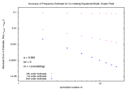
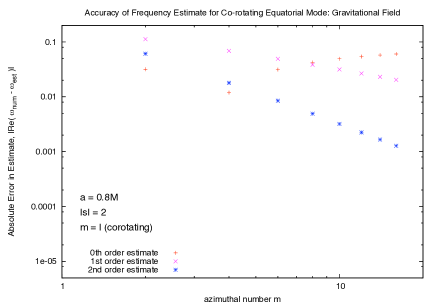
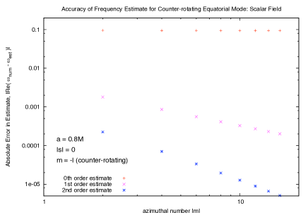
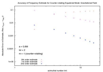
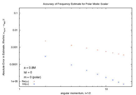
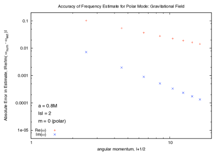
Figure 3: Accuracy of the QNM Frequency Estimates. These log-scale plots show the difference between the numerically-determined QNM frequency and the estimates obtained in this paper, as function of angular momentum $l$. The left plots show the scalar field, and the right plots show the gravitational field. The upper ($m=l$) and middle ($m=-l$) plots show the difference in the real part of the frequency, for approximations (51) and (52) truncated at orders $l^{1}$ (0th order), $l^{0}$ (1st) and $l^{-1}$ (2nd). At large $l$, the slopes of the data sets on the log-log scale approach $0$, $-1$ and $-2$, as expected. The lower plots show the difference for the real and imaginary parts of the polar ($m=0$) frequencies. The gradients tend to -1 [red, real] and -2 [blue, imaginary], implying that the approximation is accurate up to order $\mathcal{O}(L^{-1})$ for the real part and $\mathcal{O}(L^{-2})$ for the imaginary part.

IV.0.2 Polar Modes

Table 3 compares numerically-determined polar ($m=0$) frequencies for scalar and gravitational fields, with the approximation of Eq. (69). The approximation is closer to the scalar QNM frequency than to the gravitational QNM frequency. In the lower plots of Fig. 3, the error in the real and imaginary part of frequency is shown. It is clear from the gradients of the two data sets that the next-order correction to (69) is at $\mathcal{O}(l^{-1})$ for the real part, and $\mathcal{O}(l^{-2})$ for the imaginary part.

$l$		Re($M\omega$)	Im($M\omega$)
$l=2$,	scalar	0.50712267	-0.08966931
	gravitational	0.40191735	-0.08215627
	estimate	0.50478271	-0.08937858
$l=4$,	scalar	0.90990916	-0.08947052
	gravitational	0.85459105	-0.08741415
	estimate	0.90860889	-0.08937858
$l=6$,	scalar	1.31333515	-0.08942290
	gravitational	1.27557678	-0.08848090
	estimate	1.31243506	-0.08937858
$l=8$,	scalar	1.71694949	-0.08940455
	gravitational	1.68823375	-0.08886365
	estimate	1.71626123	-0.08937858
$l=10$,	scalar	2.12064455	-0.08939561
	gravitational	2.09746074	-0.08904433
	estimate	2.12008740	-0.08937858

Table 3: Polar Modes. The table compares the numerically-determined values of the ‘polar’ ($m=0$) modes (top two rows) with the lowest-order estimate (69). Note that at leading order the estimate is spin-independent.

V Discussion and Conclusions

In this paper we have obtained new closed-form approximations for the fundamental ($n=0$) Kerr QNM frequencies of the equatorial ($m=\pm l$) and polar ($m=0$) modes of arbitrary spin, valid in the regime $l\gg|s|$; see Eq. (51), (52) and (69). The result for the corotating modes improves upon previous approximations Mashhoon ; Lyapunov1 ; Hod in two regards, giving: (i) a spin-independent correction to the real part of the frequency at order $m^{0}$, (ii) a spin-dependent correction to the real part at order $m^{-1}$. The result for the polar modes is (we believe) substantially new. We demonstrated that the approximations fit the numerical data in the asymptotic regime. We have sought to improve understanding of the link between the asymptotic structure of the QNM spectrum and the properties of the unstable photon orbits (see also Goebel ; Mashhoon ; Lyapunov1 ; Hod ).

Let us conclude by suggesting some possible extensions to this work: (i) it is simple to extend the analysis to higher overtones ($n>0$) following Dolan-Ottewill ; (ii) it should be straightforward to extend the analysis to the Kerr-Newman ($Q\geq 0$) black hole (though here coupling between electromagnetic and gravitational perturbations may complicate the issue Kokkotas-1993 ; Kokkotas-Berti-2005 ); (iii) here we have considered only the limiting cases of equatorial ($|m|=l$) and polar ($m=0$) modes here; extension to general modes ($m=\mu l$, $-1\leq\mu\leq 1$) remains an open challenge. We expect the real and imaginary parts to again be linked to the orbital frequency and Lyapunov exponent on the relevant null orbit (i.e. the general orbits considered in Teo ), although we also expect some non-trivial correction at $\mathcal{O}(l^{0})$, such as appears in (51); (iv) The expansion method detailed here could also be applied to find the Regge poles of the Kerr black hole in the eikonal regime Decanini-Folacci-2010a ; Decanini-Folacci-2010b ; (v) The expansion method can also be applied to compute QNM excitation factors Leaver-1986 ; Berti-Cardoso-2006 , which are needed to tackle the question ‘how much QNM ringing is excited by a given perturbation?’ We hope to pursue this calculation in the near future.

Appendix A Period and Lyapunov Exponent for Polar Orbit

Here we derive expressions for the orbital frequency and Lyapunov exponent for the polar orbit. The period $T_{\circ}$ with respect to the coordinate time is

$$T_{\circ}=2\int_{-1}^{1}\frac{\dot{t}}{\dot{z}}\,dz,$$ (70)

where, from Eq. (3) and (6),

$$\dot{t}=\left.\frac{\Sigma^{2}}{\rho^{2}\,\Delta}\right|_{r=\hat{r}_{\circ}},\quad\quad\quad\dot{z}=\left.\rho^{-2}({d}_{\circ}^{2}+a^{2}z^{2})^{1/2}(1-z^{2})^{1/2}\right|_{r=\hat{r}_{\circ}}.$$ (71)

and ${d}_{\circ}=\sqrt{b_{\circ}-a^{2}}\equiv\sqrt{\mathcal{Q}}/E$. The $\dot{t}$ expression can be simplified with the use of the identities

$$\hat{r}_{\circ}={d}_{\circ}\left(\frac{\hat{r}_{\circ}^{2}-a^{2}}{3\hat{r}_{\circ}^{2}+a^{2}}\right)^{1/2},\quad\quad M=\hat{r}_{\circ}\left(\frac{\hat{r}_{\circ}^{2}+a^{2}}{3\hat{r}_{\circ}^{2}-a^{2}}\right),$$ (72)

to obtain

$$\dot{t}=\rho^{-2}\left({d}_{\circ}^{2}+a^{2}z^{2}\right)$$ (73)

Hence the period is

$$T_{\circ}=2\int_{-1}^{1}\frac{\left({d}_{\circ}^{2}+a^{2}z^{2}\right)^{1/2}}{\left(1-z^{2}\right)^{1/2}}dz$$ (74)

which evaluates to result (20).

The Lyapunov exponent $\lambda_{\circ}$ can be found from taking an orbital average,

$$\lambda_{\circ}=\frac{2}{T_{\circ}}\int_{-1}^{1}\bar{\lambda}\,\left(\frac{\dot{t}}{\dot{z}}\right)dz.$$ (75)

of the expression Lyapunov1 ,

$$\bar{\lambda}=\left.\dot{t}^{-1}\sqrt{\frac{1}{2}\frac{d^{2}V_{r}}{dr^{2}}}\right|_{r=\hat{r}_{\circ}}$$ (76)

where $V_{r}\equiv\dot{r}^{2}=\rho^{-4}(r-\hat{r}_{\circ})^{2}(r^{2}+2r\hat{r}_{\circ}-a^{2}{d}_{\circ}^{2}/\hat{r}_{\circ}^{2})$. Using $V_{r}^{\prime\prime}=2\rho^{-4}(3\hat{r}_{\circ}^{2}-a^{2}{d}_{\circ}^{2}/\hat{r}_{\circ}^{2})$ gives

$$\lambda_{\circ}=\frac{2(3\hat{r}_{\circ}^{2}-a^{2}{d}_{\circ}^{2}/\hat{r}_{\circ}^{2})^{1/2}}{T_{\circ}}\int_{-1}^{1}\frac{dz}{\left({d}_{\circ}^{2}+a^{2}z^{2}\right)^{1/2}\left(1-z^{2}\right)^{1/2}}.$$ (77)

which leads directly to result (22).