Statistical mechanics approach to the probability distribution of money

Abstract

This Chapter reviews statistical models for the probability distribution of money developed in the econophysics literature since the late 1990s. In these models, economic transactions are modeled as random transfers of money between the agents in payment for goods and services. Starting from the initially equal distribution of money, the system spontaneously develops a highly unequal distribution of money analogous to the Boltzmann-Gibbs distribution of energy in physics. Boundary conditions are crucial for achieving a stationary distribution. When debt is permitted, it destabilizes the system, unless some sort of limit is imposed on maximal debt.

“Money, it’s a gas.” Pink Floyd, Dark Side of the Moon

I Introduction

In this Chapter, the probability distribution of money in a system of economic agents is studied using methods of statistical physics. This study originates from the interdisciplinary field known as econophysics Stanley et al. (1996), which applies mathematical methods of statistical physics to social, economical, and financial problems Stauffer (2004).

One of the most puzzling social problems is the persistent wide range of economic inequality among the population in any society. In statistical physics, it is very well known that identical (“equal”) molecules in a gas spontaneously develop a widely unequal distribution of energies as a result of random energy transfers in collisions between the molecules. Using similar principles, this Chapter shows how a very unequal probability distribution of money among economic agents develops spontaneously as a result of money transfers between them.

The literature on social and economic inequality is enormous Kakwani (1980). Many papers in the economic literature Gibrat (1931); Kalecki (1945); Champernowne (1953) use a stochastic process to describe dynamics of individual wealth or income and to derive their probability distributions. One might call this a one-body approach, because wealth and income fluctuations are considered independently for each economic agent. Inspired by Boltzmann’s kinetic theory of collisions in gases, we introduce an alternative, two-body approach, where agents perform pairwise economic transactions and transfer money from one agent to another. We start with a simple pairwise-transfer model proposed by Drăgulescu and Yakovenko (2000). This model is the most closely related to the traditional statistical mechanics, which we briefly review first. Then we discuss other money-transfer models and further developments. For a more detailed and systematic review of the progress in this field, see the recent review by Yakovenko and Rosser (2009), as well as reviews by Richmond, Repetowicz, Hutzler, and Coelho (2006); Richmond, Hutzler, Coelho, and Repetowicz (2006); Chatterjee and Chakrabarti (2007) and a popular article by Hayes (2002).

Interestingly, the study of pairwise money transfer and the resulting statistical distribution of money have virtually no counterpart in the modern economic literature. Only the search theory of money Kiyotaki and Wright (1993) is somewhat related to it. However, a probability distribution of money among the agents within the search-theoretical approach was only recently obtained numerically by the economist Miguel Molico (2006).

II The Boltzmann-Gibbs distribution of energy

The fundamental law of equilibrium statistical mechanics is the Boltzmann-Gibbs distribution. It states that the probability $P(\varepsilon)$ of finding a physical system or subsystem in a state with the energy $\varepsilon$ is given by the exponential function

$$P(\varepsilon)=c\,e^{-\varepsilon/T},$$ (1)

where $T$ is the temperature, and $c$ is a normalizing constant Wannier (1987). Here we set the Boltzmann constant $k_{B}$ to unity by choosing the energy units for measuring the physical temperature $T$. Then, the expectation value of any physical variable $x$ can be obtained as

$$\langle x\rangle=\frac{\sum_{k}x_{k}e^{-\varepsilon_{k}/T}}{\sum_{k}e^{-\varepsilon_{k}/T}},$$ (2)

where the sum is taken over all states of the system. Temperature is equal to the average energy per particle: $T\sim\langle\varepsilon\rangle$, up to a numerical coefficient of the order of 1.

Eq. (1) can be derived in different ways Wannier (1987). All derivations involve the two main ingredients: statistical character of the system and conservation of energy $\varepsilon$. One of the shortest derivations can be summarized as follows. Let us divide the system into two (generally unequal) parts. Then, the total energy is the sum of the parts: $\varepsilon=\varepsilon_{1}+\varepsilon_{2}$, whereas the probability is the product of probabilities: $P(\varepsilon)=P(\varepsilon_{1})\,P(\varepsilon_{2})$. The only solution of these two equations is the exponential function (1).

A more sophisticated derivation, proposed by Boltzmann, uses the concept of entropy. Let us consider $N$ particles with the total energy $E$. Let us divide the energy axis into small intervals (bins) of width $\Delta\varepsilon$ and count the number of particles $N_{k}$ having the energies from $\varepsilon_{k}$ to $\varepsilon_{k}+\Delta\varepsilon$. The ratio $N_{k}/N=P_{k}$ gives the probability for a particle to have the energy $\varepsilon_{k}$. Let us now calculate the multiplicity $W$, which is the number of permutations of the particles between different energy bins such that the occupation numbers of the bins do not change. This quantity is given by the combinatorial formula in terms of the factorials

$$W=\frac{N!}{N_{1}!\,N_{2}!\,N_{3}!\,\ldots}.$$ (3)

The logarithm of multiplicity is called the entropy $S=\ln W$. In the limit of large numbers, the entropy per particle can be written in the following form using the Stirling approximation for the factorials

$$\frac{S}{N}=-\sum_{k}\frac{N_{k}}{N}\ln\left(\frac{N_{k}}{N}\right)=-\sum_{k}P_{k}\ln P_{k}.$$ (4)

Now we would like to find what distribution of particles among different energy states has the highest entropy, i.e., the highest multiplicity, provided the total energy of the system, $E=\sum_{k}N_{k}\varepsilon_{k}$, has a fixed value. Solution of this problem can be easily obtained using the method of Lagrange multipliers Wannier (1987), and the answer is given by the exponential distribution (1).

The same result can be also derived from the ergodic theory, which says that the many-body system occupies all possible states of a given total energy with equal probabilities. Then it is straightforward to show López-Ruiz et al. (2008) that the probability distribution of the energy of an individual particle is given by Eq. (1).

III Conservation of money

The derivations outlined in Sec. II are very general and only use the statistical character of the system and the conservation of energy. So, one may expect that the exponential Boltzmann-Gibbs distribution (1) would apply to other statistical systems with a conserved quantity.

The economy is a big statistical system with millions of participating agents, so it is a promising target for applications of statistical mechanics. Is there a conserved quantity in the economy? Drăgulescu and Yakovenko (2000) argued that such a conserved quantity is money $m$. Indeed, the ordinary economic agents can only receive money from and give money to other agents. They are not permitted to “manufacture” money, e.g., to print dollar bills. Let us consider an economic transaction between agents $i$ and $j$. When the agent $i$ pays money $\Delta m$ to the agent $j$ for some goods or services, the money balances of the agents change as follows

$$m_{i}\;\rightarrow\;m_{i}^{\prime}=m_{i}-\Delta m,$$

$$m_{j}\;\rightarrow\;m_{j}^{\prime}=m_{j}+\Delta m.$$ (5)

The total amount of money of the two agents before and after transaction remains the same

$$m_{i}+m_{j}=m_{i}^{\prime}+m_{j}^{\prime},$$ (6)

i.e., there is a local conservation law for money. The rule (5) for the transfer of money is analogous to the transfer of energy from one molecule to another in molecular collisions in a gas, and Eq. (6) is analogous to conservation of energy in such collisions. Conservative models of this kind are also studied in some economic literature Kiyotaki and Wright (1993); Molico (2006).

We should emphasize that, in the model of Drăgulescu and Yakovenko (2000) [as in the economic models of Kiyotaki and Wright (1993); Molico (2006)], the transfer of money from one agent to another represents payment for goods and services in a market economy. However, the model of Drăgulescu and Yakovenko (2000) only keeps track of money flow, but does not keep track of what goods and service are delivered. One reason for this is that many goods, e.g., food and other supplies, and most services, e.g., getting a haircut or going to a movie, are not tangible and disappear after consumption. Because they are not conserved, and also because they are measured in different physical units, it is not very practical to keep track of them. In contrast, money is measured in the same unit (within a given country with a single currency) and is conserved in local transactions (6), so it is straightforward to keep track of money flow. It is also important to realize that an increase in material production does not produce an automatic increase in money supply. The agents can grow apples on trees, but cannot grow money on trees. Only a central bank has the monopoly of changing the monetary base $M_{b}$ McConnell and Brue (1996). (Debt and credit issues are discussed separately in Sec. VI.)

Enforcement of the local conservation law (6) is the key feature for successful functioning of money. If the agents were permitted to “manufacture” money, they would be printing money and buying all goods for nothing, which would be a disaster. The purpose of the conservation law is to ensure that an agent can buy goods and products from the society (the other agents) only if he or she contributes something useful to the society and receives money payment for these contributions. Thus, money is an accounting device, and, indeed, all accounting systems are based on the conservation law (5). The physical medium of money is not essential as long as the local conservation law is enforced. The days of gold standard are long gone, so money today is truly the fiat money, declared to be money by the central bank. Money may be in the form of paper currency, but today it is more often represented by digits on computerized accounts. So, money is nothing but bits of information, and monetary system represents an informational layer of the economy. Monetary system interacts with physical system (production and consumption of material goods), but the two layers cannot be transformed into each other because of their different nature.

Unlike, ordinary economic agents, a central bank or a central government can inject money into the economy, thus changing the total amount of money in the system. This process is analogous to an influx of energy into a system from external sources, e.g., the Earth receives energy from the Sun. Dealing with these situations, physicists start with an idealization of a closed system in thermal equilibrium and then generalize to an open system subject to an energy flux. As long as the rate of money influx from central sources is slow compared with relaxation processes in the economy and does not cause hyperinflation, the system is in quasi-stationary statistical equilibrium with slowly changing parameters. This situation is analogous to heating a kettle on a gas stove slowly, where the kettle has a well-defined, but slowly increasing, temperature at any moment of time. A flux of money may be also produced by international transfers across the boundaries of a country. This process involves complicated issues of multiple currencies in the world and their exchange rates McCauley (2008). Here we consider an idealization of a closed economy for a single country with a single currency.

Another potential problem with conservation of money is debt. This issue will be discussed in Sec. VI. As a starting point, Drăgulescu and Yakovenko (2000) considered simple models, where debt is not permitted, which is also a common idealization in some economic literature Kiyotaki and Wright (1993); Molico (2006). This means that money balances of the agents cannot go below zero: $m_{i}\geq 0$ for all $i$. Transaction (5) takes place only when an agent has enough money to pay the price: $m_{i}\geq\Delta m$, otherwise the transaction does not take place. If an agent spends all money, the balance drops to zero $m_{i}=0$, so the agent cannot buy any goods from other agents. However, this agent can still receive money from other agents for delivering goods or services to them. In real life, money balance dropping to zero is not at all unusual for people who live from paycheck to paycheck.

Macroeconomic monetary policy issues, such as money supply and money demand Friedman and Hahn (1990), are outside of the scope of this Chapter. Our goal is to investigate the probability distribution of money among economic agents. For this purpose, it is appropriate to make the simplifying macroeconomic idealizations, as described above, in order to ensure overall stability of the system and existence of statistical equilibrium. The concept of “equilibrium” is a very common idealization in economic literature, even though the real economies might never be in equilibrium. Here we extend this concept to a statistical equilibrium, which is characterized by a stationary probability distribution of money $P(m)$, in contrast to a mechanical equilibrium, where the “forces” of demand and supply balance each other.

IV The Boltzmann-Gibbs distribution of money

Having recognized the principle of local money conservation, Drăgulescu and Yakovenko (2000) argued that the stationary distribution of money $P(m)$ should be given by the exponential Boltzmann-Gibbs function analogous to Eq. (1)

$$P(m)=c\,e^{-m/T_{m}}.$$ (7)

Here $c$ is a normalizing constant, and $T_{m}$ is the “money temperature”, which is equal to the average amount of money per agent: $T=\langle m\rangle=M/N$, where $M$ is the total money, and $N$ is the number of agents.

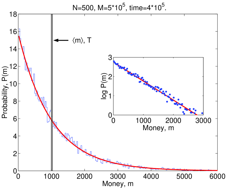
Figure 1: Histogram and points: Stationary probability distribution of money $P(m)$ obtained in additive random-exchange models. Solid curves: Fits to the exponential Boltzmann-Gibbs law (7). Vertical line: The initial distribution of money. From Drăgulescu and Yakovenko (2000).

To verify this conjecture, Drăgulescu and Yakovenko (2000) performed agent-based computer simulations of money transfers between agents. Initially all agents were given the same amount of money, say, $1000. Then, a pair of agents $(i,j)$ was randomly selected, the amount $\Delta m$ was transferred from one agent to another, and the process was repeated many times. Time evolution of the probability distribution of money $P(m)$ is illustrated in computer animation videos by Chen and Yakovenko (2007) and by Wright (2007). After a transitory period, money distribution converges to the stationary form shown in Fig. 1. As expected, the distribution is well fitted by the exponential function (7).

Several different rules for $\Delta m$ were considered by Drăgulescu and Yakovenko (2000). In one model, the transferred amount was fixed to a constant $\Delta m=\$1$. Economically, it means that all agents were selling their products for the same price $\Delta m=\$1$. Computer animation Chen and Yakovenko (2007) shows that the initial distribution of money first broadens to a symmetric Gaussian curve, characteristic for a diffusion process. Then, the distribution starts to pile up around the $m=0$ state, which acts as the impenetrable boundary, because of the imposed condition $m\geq 0$. As a result, $P(m)$ becomes skewed (asymmetric) and eventually reaches the stationary exponential shape, as shown in Fig. 1. The boundary at $m=0$ is analogous to the ground-state energy in statistical physics. Without this boundary condition, the probability distribution of money would not reach a stationary state. Computer animations Chen and Yakovenko (2007); Wright (2007) also show how the entropy of money distribution, defined as $S/N=-\sum_{k}P(m_{k})\ln P(m_{k})$, grows from the initial value $S=0$, where all agents have the same money, to the maximal value at the statistical equilibrium.

While the model with $\Delta m=1$ is very simple and instructive, it is not realistic, because all prices are taken to be the same. In another model considered by Drăgulescu and Yakovenko (2000), $\Delta m$ in each transaction is taken to be a random fraction of the average amount of money per agent, i.e., $\Delta m=\nu(M/N)$, where $\nu$ is a uniformly distributed random number between 0 and 1. The random distribution of $\Delta m$ is supposed to represent the wide variety of prices for different products in the real economy. Computer simulation of this model produces the same stationary distribution (7). Drăgulescu and Yakovenko (2000) also considered a model with firms, which hire agents to produce and sell products. This process results in a many-body transfer of money, as opposed to pairwise transfer discussed above. Computer simulation of this model also generates the same exponential distribution (7).

These ideas were further developed by Scalas et al. (2006); Garibaldi et al. (2007). The Boltzmann distribution was independently applied to social sciences by the physicist Jürgen Mimkes (2000); Mimkes and Willis (2005) using the Lagrange principle of maximization with constraints. The exponential distribution of money was also found by the economist Martin Shubik (1999) using a Markov chain approach to strategic market games. A long time ago, Benoit Mandelbrot (1960, p 83) observed:

“There is a great temptation to consider the exchanges of money which occur in economic interaction as analogous to the exchanges of energy which occur in physical shocks between gas molecules.”

He realized that this process should result in the exponential distribution, by analogy with the barometric distribution of density in the atmosphere. However, he discarded this idea, because it does not produce the Pareto power law Pareto (1897), and proceeded to study the stable Lévy distributions. Ironically, the actual economic data Yakovenko and Rosser (2009) do show the exponential distribution for the majority of the population. Moreover, the data have a finite variance, so the stable Lévy distributions are not applicable because of their infinite variance.

V Proportional money transfers and saving propensity

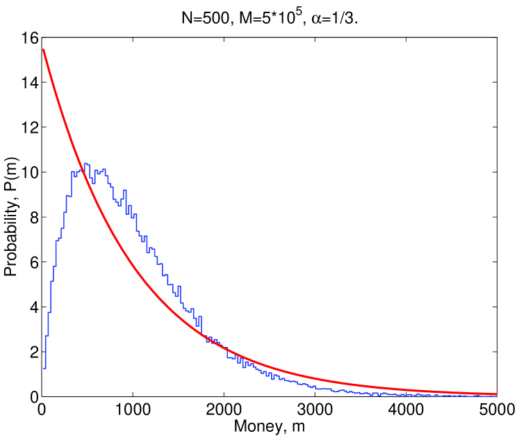
Figure 2: Histogram: Stationary probability distribution of money in the multiplicative random-exchange model (8) for $\gamma=1/3$. Solid curve: The exponential Boltzmann-Gibbs law. From Drăgulescu and Yakovenko (2000).

In the models of money transfer discussed in Sec. IV, the transferred amount $\Delta m$ is typically independent of the money balances of the agents involved. A different model was introduced earlier by the physicists Ispolatov, Krapivsky, and Redner (1998) and called the multiplicative asset exchange model. This model also satisfies the conservation law, but the transferred amount of money is a fixed fraction $\gamma$ of the payer’s money in Eq. (5):

$$\Delta m=\gamma m_{i}.$$ (8)

The stationary distribution of money in this model, compared in Fig. 2 with an exponential function, is similar, albeit not exactly equal, to the Gamma distribution:

$$P(m)=c\,m^{\beta}\,e^{-m/T}.$$ (9)

Eq. (9) differs from Eq. (7) by the power-law prefactor $m^{\beta}$. For $\beta>0$, the population with low money balances is reduced, and $P(0)=0$, as shown in Fig. 2.

Essentially the same model Lux (2005), called the inequality process, has been introduced and studied much earlier by the sociologist John Angle (1986, 1992, 1993, 1996, 2002, 2006). Angle (1986) associated the proportionality rule (8) with the surplus theory of social stratification Engels (1972), which argues that inequality in human society develops when people can produce more than necessary for minimal subsistence. This additional wealth (surplus) can be transferred from original producers to other people, thus generating inequality. Angle found a Gamma-like distribution (9) in numerical simulations of his models. Independently, the economist Miguel Molico (2006) studied conservative exchange models (5) where agents bargain over prices in their transactions. He also found a stationary Gamma-like distribution of money in numerical simulations.

Another model with an element of proportionality was proposed by Chakraborti and Chakrabarti (2000). In this model, the agents set aside (save) some fraction of their money $\lambda m_{i}$, whereas the rest of their money balance $(1-\lambda)m_{i}$ becomes available for random exchanges. Thus, the rule of exchange (5) becomes

$$m_{i}^{\prime}=\lambda m_{i}+\xi(1-\lambda)(m_{i}+m_{j}),$$

$$m_{j}^{\prime}=\lambda m_{j}+(1-\xi)(1-\lambda)(m_{i}+m_{j}).$$ (10)

Here the coefficient $\lambda$ is called the saving propensity, and the random variable $\xi$ is uniformly distributed between 0 and 1. Computer simulations by Chakraborti and Chakrabarti (2000) of the model (10) found a stationary distribution close to the Gamma distribution (9). With $\lambda\neq 0$, agents always keep some money, so their balances never drop to zero, thus $P(0)=0$.

In the subsequent papers by the Kolkata school and related papers, the case of random saving propensity was studied. In these models, the agents are assigned random parameters $\lambda$ drawn from a uniform distribution between 0 and 1 Chatterjee, Chakrabarti, and Manna (2004). It was found that this model produces a power-law tail $P(m)\propto 1/m^{2}$ at high $m$. The reasons for stability of this law were understood using the Boltzmann kinetic equation Das and Yarlagadda (2005); Chatterjee, Chakrabarti, and Stinchcombe (2005); Repetowicz, Hutzler, and Richmond (2005), but most elegantly in the mean-field theory Mohanty (2006); Bhattacharyya, Chatterjee, and Chakrabarti (2007); Chatterjee and Chakrabarti (2007). The fat tail originates from the agents whose saving propensity is close to 1, who hoard money and do not give it back Patriarca et al. (2005); Patriarca, Chakraborti, and Germano (2006). A more rigorous mathematical treatment of the problem was given by Düring, Matthes, and Toscani (2008); Matthes and Toscani (2008); Düring and Toscani (2007).

As a further extension, Drăgulescu and Yakovenko (2000) considered a model with taxation, which also has an element of proportionality. The Gamma distribution was also studied for conservative models within a simple Boltzmann approach by Ferrero (2004, 2005) and, using more complicated rules of exchange motivated by political economy, by Scafetta, Picozzi, and West (2004a, b). Another extension of these studies includes not only money transfers, but also transfers of a commodity, for which money is paid Chakraborti, Pradhan, and Chakrabarti (2001); Chatterjee and Chakrabarti (2006); Ausloos and Pekalski (2007); Silver, Slud, and Takamoto (2002); Lux (2009). For a more detailed review of these models, see Yakovenko and Rosser (2009).

The stationary distribution of money (9) is different from the simple exponential formula (7). The origin of this difference can be understood from the Boltzmann kinetic equation Wannier (1987); Lifshitz and Pitaevskii (1981). This equation describes time evolution of the distribution function $P(m)$ due to pairwise interactions:

$$\frac{dP(m)}{dt}=\int\!\!\!\!\int\{-f_{[m,m^{\prime}]\to[m-\Delta,m^{\prime}+\Delta]}P(m)P(m^{\prime})$$ (11)

$$+f_{[m-\Delta,m^{\prime}+\Delta]\to[m,m^{\prime}]}P(m-\Delta)P(m^{\prime}+\Delta)\}\,dm^{\prime}\,d\Delta.$$

Here $f_{[m,m^{\prime}]\to[m-\Delta,m^{\prime}+\Delta]}$ is the probability of transferring money $\Delta$ from an agent with money $m$ to an agent with money $m^{\prime}$ per unit time. This probability, multiplied by the occupation numbers $P(m)$ and $P(m^{\prime})$, gives the rate of transitions from the state $[m,m^{\prime}]$ to the state $[m-\Delta,m^{\prime}+\Delta]$. The first term in Eq. (11) gives the depopulation rate of the state $m$. The second term in Eq. (11) describes the reversed process, where the occupation number $P(m)$ increases. When the two terms are equal, the direct and reversed transitions cancel each other statistically, and the probability distribution is stationary: $dP(m)/dt=0$. This is the principle of detailed balance.

In physics, the fundamental microscopic equations of motion obey the time-reversal symmetry. This means that the probabilities of the direct and reversed processes are exactly equal:

$$f_{[m,m^{\prime}]\to[m-\Delta,m^{\prime}+\Delta]}=f_{[m-\Delta,m^{\prime}+\Delta]\to[m,m^{\prime}]}.$$ (12)

When Eq. (12) is satisfied, the detailed balance condition for Eq. (11) reduces to the equation $P(m)P(m^{\prime})=P(m-\Delta)P(m^{\prime}+\Delta)$, because the factors $f$ cancels out. The only solution of this equation is the exponential function $P(m)=c\exp(-m/T_{m})$, so the Boltzmann-Gibbs distribution is the stationary solution of the Boltzmann kinetic equation (11). Notice that the transition probabilities (12) are determined by the dynamical rules of the model, but the equilibrium Boltzmann-Gibbs distribution does not depend on the dynamical rules at all. This is the origin of the universality of the Boltzmann-Gibbs distribution. We see that it is possible to find the stationary distribution without knowing details of the dynamical rules (which are rarely known very well), as long as the symmetry condition (12) is satisfied.

The models considered in Sec. IV have the time-reversal symmetry. The model with the fixed money transfer $\Delta$ has equal probabilities (12) of transferring money from an agent with the balance $m$ to an agent with the balance $m^{\prime}$ and vice versa. This is also true when $\Delta$ is random, as long as the probability distribution of $\Delta$ is independent of $m$ and $m^{\prime}$. Thus, the stationary distribution $P(m)$ is always exponential in these models. On the other hand, in the model (8), the time-reversal symmetry is broken. Indeed, when an agent $i$ gives a fixed fraction $\gamma$ of his money $m_{i}$ to an agent with balance $m_{j}$, their balances become $(1-\gamma)m_{i}$ and $m_{j}+\gamma m_{i}$. If we try to reverse this process and appoint the agent $j$ to be the payer and to give the fraction $\gamma$ of her money, $\gamma(m_{j}+\gamma m_{i})$, to the agent $i$, the system does not return to the original configuration $[m_{i},m_{j}]$. As emphasized by Angle (2006), the payer pays a deterministic fraction of his money, but the receiver receives a random amount from a random agent, so their roles are not interchangeable. Because the proportional rule typically violates the time-reversal symmetry, the stationary distribution $P(m)$ in multiplicative models is not exponential.

These examples show that the Boltzmann-Gibbs distribution does not necessarily hold for any conservative model. However, it is universal in a limited sense for a broad class of models that have time-reversal symmetry. In the absence of detailed knowledge of real microscopic dynamics of economic exchanges, the semiuniversal Boltzmann-Gibbs distribution (7) is a natural starting point. Moreover, the assumption of Drăgulescu and Yakovenko (2000) that agents pay the same prices $\Delta m$ for the same products, independent of their money balances $m$, seems very appropriate for the modern anonymous economy, especially for purchases over the Internet. There is no particular empirical evidence for the proportional rules (8) or (10). By further modifying the rules of money transfer and introducing more parameters in the models, it is possible to obtain even more complicated distributions Scafetta and West (2007). However, parsimony is the virtue of a good mathematical model, not the abundance of additional assumptions and parameters, whose correspondence to reality is hard to verify.

VI Models with debt

Now let us discuss how the results change when debt is permitted. From the standpoint of individual economic agents, debt may be considered as negative money. When an agent borrows money from a bank (considered here as a big reservoir of money), the cash balance of the agent (positive money) increases, but the agent also acquires a debt obligation (negative money), so the total balance (net worth) of the agent remains the same. Thus, the act of borrowing money still satisfies a generalized conservation law of the total money (net worth), which is now defined as the algebraic sum of positive (cash $M$) and negative (debt $D$) contributions: $M-D=M_{b}$, where $M_{b}$ is the original amount of money in the system, the monetary base McConnell and Brue (1996). After spending some cash in pairwise transactions (5), the agent still has the debt obligation (negative money), so the total money balance $m_{i}$ of the agent (net worth) becomes negative. We see that the boundary condition $m_{i}\geq 0$, discussed in Sec. III, does not apply when debt is permitted, so $m=0$ is not the ground state any more. The consequence of permitting debt is not a violation of the conservation law (which is still preserved in the generalized form for net worth), but a modification of the boundary condition by permitting agents to have negative balances $m_{i}<0$ of net worth. A more detailed discussion of positive and negative money and the book-keeping accounting from the econophysics point of view was presented by the physicist Dieter Braun (2001) and Fischer and Braun (2003a, b).

Now we can repeat the simulation described in Sec. IV without the boundary condition $m\geq 0$ by allowing agents to go into debt. When an agent needs to buy a product at a price $\Delta m$ exceeding his money balance $m_{i}$, the agent is now permitted to borrow the difference from a bank and, thus, to buy the product. As a result of this transaction, the new balance of the agent becomes negative: $m_{i}^{\prime}=m_{i}-\Delta m<0$. Notice that the local conservation law (5) and (6) is still satisfied, but it involves negative values of $m$. If the simulation is continued further without any restrictions on the debt of the agents, the probability distribution of money $P(m)$ never stabilizes, and the system never reaches a stationary state. As time goes on, $P(m)$ keeps spreading in a Gaussian manner unlimitedly toward $m=+\infty$ and $m=-\infty$. Because of the generalized conservation law discussed above, the first moment $\langle m\rangle=M_{b}/N$ of the algebraically defined money $m$ remains constant. It means that some agents become richer with positive balances $m>0$ at the expense of other agents going further into debt with negative balances $m<0$, so that $M=M_{b}+D$.

Common sense, as well as the experience with the current financial crisis, tells us that an economic system cannot be stable if unlimited debt is permitted. In this case, agents can buy any goods without producing anything in exchange by simply going into unlimited debt. Arguably, the current financial crisis was caused by the enormous debt accumulation in the system, triggered by subprime mortgages and financial derivatives based on them. A widely expressed opinion is that the current crisis is not the problem of liquidity, i.e., a temporary difficulty in cash flow, but the problem of insolvency, i.e., the inherent inability of many participants to pay back their debts.

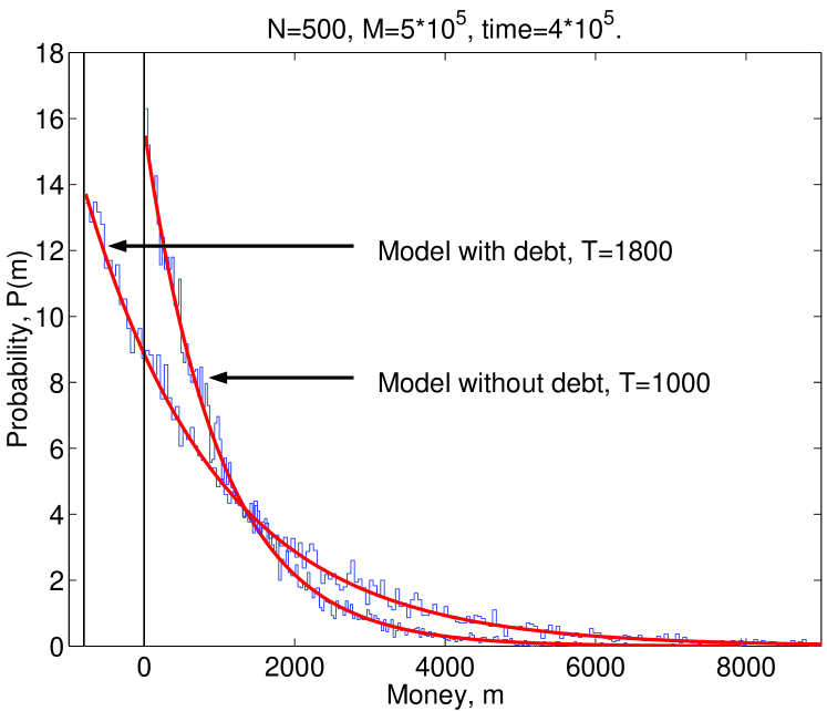
Figure 3: Histograms: Stationary distributions of money with and without debt. The debt is limited to $m_{d}=800$. Solid curves: Fits to the Boltzmann-Gibbs laws with the “money temperatures” $T_{m}=1800$ and $T_{m}=1000$. From Drăgulescu and Yakovenko (2000).

Detailed discussion of the current economic situation is not a subject of this paper. Going back to the idealized model of money transfers, one would need to impose some sort of modified boundary conditions in order to prevent unlimited growth of debt and to ensure overall stability of the system. Drăgulescu and Yakovenko (2000) considered a simple model where the maximal debt of each agent is limited to a certain amount $m_{d}$. This means that the boundary condition $m_{i}\geq 0$ is now replaced by the condition $m_{i}\geq-m_{d}$ for all agents $i$. Setting interest rates on borrowed money to be zero for simplicity, Drăgulescu and Yakovenko (2000) performed computer simulations of the models described in Sec. IV with the new boundary condition. The results are shown in Fig. 3. Not surprisingly, the stationary money distribution again has the exponential shape, but now with the new boundary condition at $m=-m_{d}$ and the higher money temperature $T_{d}=m_{d}+M_{b}/N$. By allowing agents to go into debt up to $m_{d}$, we effectively increase the amount of money available to each agent by $m_{d}$. So, the money temperature, which is equal to the average amount of effectively available money per agent, increases correspondingly.

Xi, Ding, and Wang (2005) considered another, more realistic boundary condition, where a constraint is imposed not on the individual debt of each agent, but on the total debt of all agents in the system. This is accomplished via the required reserve ratio $R$, which is briefly explained below McConnell and Brue (1996). Banks are required by law to set aside a fraction $R$ of the money deposited into bank accounts, whereas the remaining fraction $1-R$ can be loaned further. If the initial amount of money in the system (the money base) is $M_{b}$, then, with repeated loans and borrowing, the total amount of positive money available to the agents increases to $M=M_{b}/R$, where the factor $1/R$ is called the money multiplier McConnell and Brue (1996). This is how “banks create money”. Where does this extra money come from? It comes from the increase in the total debt in the system. The maximal total debt is given by $D=M_{b}/R-M_{b}$ and is limited by the factor $R$. When the debt is maximal, the total amounts of positive, $M_{b}/R$, and negative, $M_{b}(1-R)/R$, money circulate among the agents in the system, so there are two constraints in the model considered by Xi, Ding, and Wang (2005). Thus, we expect to see the exponential distributions of positive and negative money characterized by two different temperatures: $T_{+}=M_{b}/RN$ and $T_{-}=M_{b}(1-R)/RN$. This is exactly what was found in computer simulations by Xi, Ding, and Wang (2005), as shown in Fig. 4. Similar two-sided distributions were also found by Fischer and Braun (2003a).

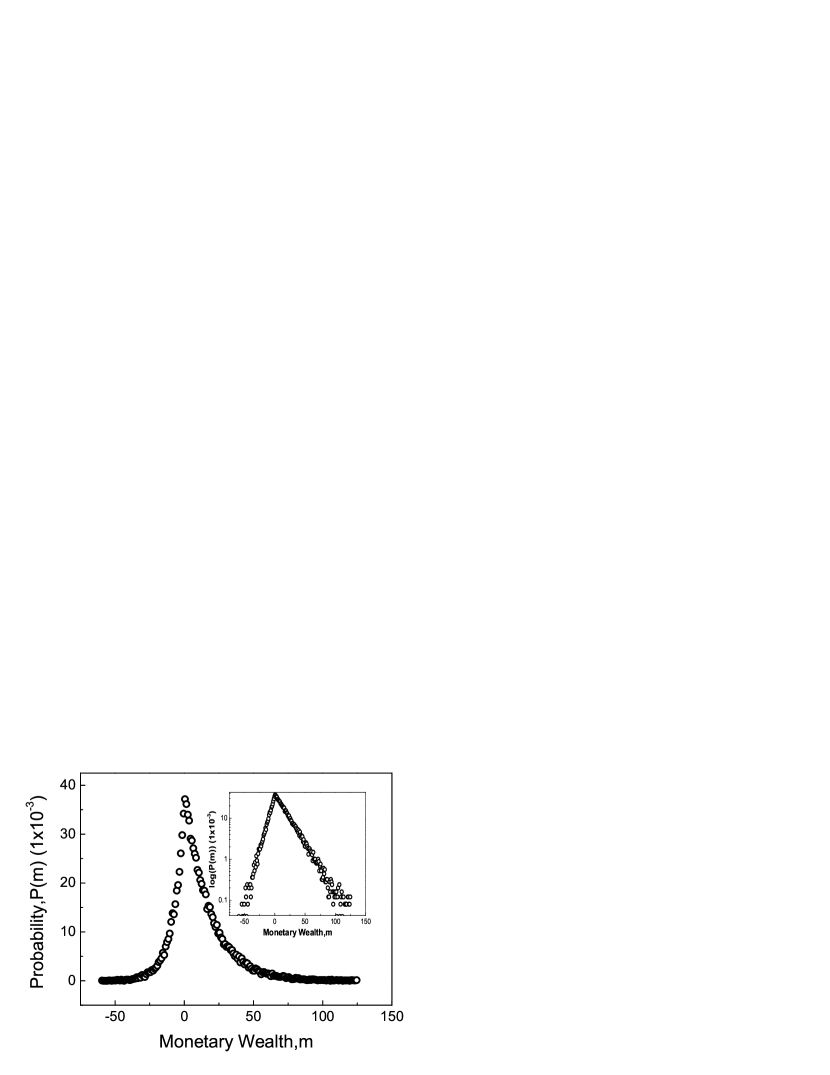
Figure 4: The stationary distribution of money for the required reserve ratio $R=0.8$. The distribution is exponential for both positive and negative money with different “temperatures” $T_{+}$ and $T_{-}$, as illustrated by the inset on log-linear scale. From Xi, Ding, and Wang (2005).

However, in the real economy, the reserve requirement is not effective in stabilizing total debt in the system, because it applies only to deposits from general public, but not from corporations. Moreover, there are alternative instruments of debt, including derivatives and various unregulated “financial innovations”. As a result, the total debt is not limited in practice and can potentially reach catastrophic proportions. Here we briefly discuss several models with non-stationary debt. Thus far, we did not consider the interest rates. Drăgulescu and Yakovenko (2000) studied a simple model with different interest rates for deposits into and loans from a bank. Computer simulations found that money distribution among the agents is still exponential, but the money temperature slowly changes in time. Depending on the choice of parameters, the total amount of money in circulation either increases or decreases in time. Interest amplifies destabilizing effect of debt, because positive balances become even more positive and negative even more negative due to accruement of interest. A more sophisticated macroeconomic model studied by the economist Steve Keen (1995, 2000) exhibits debt-induced breakdown, where all economic activity stops under the burden of heavy debt and cannot be restarted without a “debt moratorium”. The interest rates were fixed in these models and not adjusted self-consistently. Cockshott and Cottrell (2008) proposed a mechanism, where the interest rates are set to cover probabilistic withdrawals of deposits from a bank. In an agent-based simulation of the model, Cockshott and Cottrell (2008) found that money supply first increases up to a certain limit, and then the economy experiences a spectacular crash under the weight of accumulated debt.

In the absence of a nominal limit on maximal debt, bankruptcy provides a mechanism for debt stabilization. When the debt of an agent becomes too large, the agent will not be able to borrow any more money and will not be able to pay the debt back, so he or she will have to declare bankruptcy. Bankruptcy erases the debt of the agent (the negative money) and resets the balance to zero. However, somebody else (a bank or a lender) counted this debt as a positive asset, which also becomes erased. In the language of physics, creation of debt is analogous to particle-antiparticle generation (creation of positive and negative money), whereas cancellation of debt by repayment or by bankruptcy corresponds to particle-antiparticle annihilation (annihilation of positive and negative money). The former process dominates during economic bubbles (booms) and represents monetary expansion, whereas the latter dominates during the subsequent recessions (busts) and represents monetary contraction. Bankruptcy is the crucial mechanism for stabilizing money distribution, but it is often overlooked by the economists. Interest rates are meaningless without a mechanism specifying when bankruptcy is triggered.

After lending money out, the lender has the burden of collecting the debt from the debtor. Thus, the act of lending creates a persistent link (a string) between the lender and the borrower, as emphasized in the Chapter by Heiner Ganssmann in this Volume. This is in contrast to payments by positive money for goods and services, which are final and do not leave any persistent link between the agents after the transaction. Invention of the infamous collateralized debt obligations (CDO) obscured connections between lenders and borrowers by randomizing and anonymizing their pools. It destabilized the system by inviting unsustainable debt and made bankruptcy proceedings extremely difficult because of the scrambled identities of lenders and borrowers.

As argued above, boundary conditions are crucial for stabilizing money distribution. Typically, a lower bound is imposed, but not an upper bound (in a capitalist, as opposed to a socialist, society). This asymmetry is very important for stability of a monetary system. Numerous attempts were made to create alternative community money from scratch and most of them failed. In such a system, when an agent provides goods or services to another agent, their accounts are credited with positive and negative tokens, as in Eq. (5). However, because the initial global money balance is zero in this case, the probability distribution of money $P(m)$ is symmetric with respect to positive and negative $m$. Unless a boundary condition is imposed on the lower side, $P(m)$ will never stabilize. Some agents will accumulate unlimited negative balance by consuming goods and services and not contributing anything in return, thus undermining the system. In contrast, when a central government creates positive money by fiat and forces its usage by demanding that taxes are paid with this money, it creates a viable monetary system, as discussed in the Chapter by Randall Wray in this Volume. Thus, taxation is an essential ingredient for vitality of a monetary system.

VII Conclusions and perspectives

In this Chapter, we have demonstrated that random transfers of money in economic transactions between otherwise equal economic agents produce a broad and highly unequal probability distribution of money among the agents. In additive models, the probability distribution of money is exponential and similar to the Boltzmann-Gibbs distribution of energy in statistical physics. Multiplicative models produce a Gamma-like distribution and a power-law tail for random saving propensity. Local conservation of money in transactions between agents is crucial for the accounting function of money. Ordinary economic agents can only receive and give money, but cannot produce it. Boundary conditions are necessary in order to achieve a stable probability distribution of money. Without debt, zero money balance is the boundary. When debt is permitted, some sort of restriction on the negative money balances must be imposed, either by limiting individual or collective debt or by setting up conditions for bankruptcy. When debt is unlimited, the system is unstable and does not have a stationary state.

It would be very interesting to compare these theoretical conclusions with empirical data on money distribution. Unfortunately, it is very difficult to obtain such data. The probability distribution of balances on deposit accounts in a big enough bank would be a reasonable approximation for money distribution among the population. However, such data are not publicly available. In contrast, plenty of data are available on income distribution from the tax agencies. Quantitative analysis of such data for the USA Yakovenko and Rosser (2009) shows that the population consists of two distinct social classes. Income distribution follows the exponential law for the lower class (about 97% of population) and the power law for the upper class (about 3% of population). Although social classes have been known since Karl Marx, it is interesting that they can be recognized by fitting the empirical data with simple mathematical functions. Using sophisticated models of interacting economic agents, the computer scientist Ian Wright (2005, 2009) demonstrated emergence of two classes in agent-based simulations of initially equal agents. This work has been further developed in the book by Cockshott, Cottrell, Michaelson, Wright, and Yakovenko (2009), integrating economics, computer science, and physics.

Nowadays, money is typically represented by data bits on computer accounts, which constitute the informational layer of the economy. In contrast, material standards of living are determined by the physical layer of the economy. In the modern society, physical standards of living are largely determined by the level of energy consumption and are widely different around the globe. Banerjee and Yakovenko (2010) found that the probability distribution of energy consumption per capita around the world approximately follows the exponential law. So, it is likely that the energy consumption inequality is governed by the same principles as the money inequality. The energy/ecology and financial/economic crises are the biggest challenges faced by the mankind today. There is an urgent need to find ways for a manageable and realistic transition from the current breakneck growth-oriented economy, powered by ever-expanding use of fossil energy fuels, to a stable and sustainable society, based on renewable energy and balance with the Nature. Undoubtedly, both money and energy will be the key factors shaping up the future of human civilization.

References

- Angle (1986) Angle, J., 1986, “The surplus theory of social stratification and the size distribution of personal wealth,” Social Forces 65, 293–326.
- Angle (1992) Angle, J., 1992, “The inequality process and the distribution of income to blacks and whites,” Journal of Mathematical Sociology 17, 77–98.
- Angle (1993) Angle, J., 1993, “Deriving the size distribution of personal wealth from ‘the rich get richer, the poor get poorer’,” Journal of Mathematical Sociology 18, 27–46.
- Angle (1996) Angle, J., 1996, “How the Gamma Law of income distribution appears invariant under aggregation,” Journal of Mathematical Sociology 21, 325–358.
- Angle (2002) Angle, J., 2002, “The statistical signature of pervasive competition on wage and salary incomes,” Journal of Mathematical Sociology 26, 217–270.
- Angle (2006) Angle, J., 2006, “The Inequality Process as a wealth maximizing process,” Physica A 367, 388–414.
- Ausloos and Pekalski (2007) Ausloos, M., and A. Pekalski, 2007, “Model of wealth and goods dynamics in a closed market,” Physica A 373, 560–568.
- Banerjee and Yakovenko (2010) Banerjee, A., and V. M. Yakovenko, 2010, “Universal patterns of inequality,” to be published in New Journal of Physics, arXiv:0912.4898.
- Bhattacharyya, Chatterjee, and Chakrabarti (2007) Bhattacharyya, P., A. Chatterjee, and B. K. Chakrabarti, 2007, “A common mode of origin of power laws in models of market and earthquake,” Physica A 381, 377–382.
- Braun (2001) Braun, D., 2001, “Assets and liabilities are the momentum of particles and antiparticles displayed in Feynman-graphs,” Physica A 290, 491–500.
- Chakrabarti, Chakraborti, and Chatterjee (2006) Chakrabarti, B. K., A. Chakraborti, and A. Chatterjee, 2006, Eds., Econophysics and Sociophysics: Trends and Perspectives (Wiley-VCH, Berlin).
- Chakraborti and Chakrabarti (2000) Chakraborti A., and B. K. Chakrabarti, 2000, “Statistical mechanics of money: how saving propensity affects its distribution,” The European Physical Journal B 17, 167–170.
- Chakraborti, Pradhan, and Chakrabarti (2001) Chakraborti, A., S. Pradhan, and B. K. Chakrabarti, 2001, “A self-organising model of market with single commodity,” Physica A 297, 253–259.
- Champernowne (1953) Champernowne, D. G., 1953, “A model of income distribution,” The Economic Journal 63, 318–351.
- Chatterjee and Chakrabarti (2006) Chatterjee, A., and B. K. Chakrabarti, 2006, “Kinetic market models with single commodity having price fluctuations,” The European Physical Journal B 54, 399–404.
- Chatterjee and Chakrabarti (2007) Chatterjee, A., and B. K. Chakrabarti, 2007, “Kinetic exchange models for income and wealth distributions,” The European Physical Journal B 60, 135–149.
- Chatterjee, Chakrabarti, and Manna (2004) Chatterjee, A., B. K. Chakrabarti, and S. S. Manna, 2004, “Pareto law in a kinetic model of market with random saving propensity,” Physica A 335, 155-163.
- Chatterjee, Chakrabarti, and Stinchcombe (2005) Chatterjee, A., B. K. Chakrabarti, and R. B. Stinchcombe, 2005, “Master equation for a kinetic model of a trading market and its analytic solution,” Physical Review E 72, 026126.
- Chatterjee, Yarlagadda, and Chakrabarti (2005) Chatterjee, A., S. Yarlagadda, and B. K. Chakrabarti, 2005, Eds., Econophysics of Wealth Distributions (Springer, Milan).
- Chen and Yakovenko (2007) Chen, J., and V. M. Yakovenko, 2007, Computer animation videos of money-transfer models, http://www2.physics.umd.edu/~yakovenk/econophysics/animation.html.
- Cockshott and Cottrell (2008) Cockshott, P., and A. Cottrell, 2008, “Probabilistic political economy and endogenous money,” talk presented at the conference Probabilistic Political Economy, Kingston University (UK), July 2008, available at http://www.dcs.gla.ac.uk/publications/PAPERS/8935/probpolecon.pdf.
- Cockshott, Cottrell, Michaelson, Wright, and Yakovenko (2009) Cockshott, W. P., A. F. Cottrell, G. J. Michaelson, I. P. Wright, and V. M. Yakovenko, 2009, Classical Econophysics (Routledge, Oxford).
- Das and Yarlagadda (2005) Das, A., and S. Yarlagadda, 2005, “An analytic treatment of the Gibbs-Pareto behavior in wealth distribution,” Physica A 353, 529–538.
- Drăgulescu and Yakovenko (2000) Drăgulescu, A. A., and V. M. Yakovenko, 2000, “Statistical mechanics of money,” The European Physical Journal B 17, 723–729.
- Düring, Matthes, and Toscani (2008) Düring, B., D. Matthes, and G. Toscani, 2008, “Kinetic equations modelling wealth redistribution: A comparison of approaches,” Physical Review E 78, 056103.
- Düring and Toscani (2007) Düring, B., and G. Toscani, 2007, “Hydrodynamics from kinetic models of conservative economies,” Physica A 384, 493–506.
- Engels (1972) Engels, F., 1972, The Origin of the Family, Private Property and the State, in the Light of the Researches of Lewis H. Morgan (International Publishers, New York).
- Ferrero (2004) Ferrero, J. C., 2004, “The statistical distribution of money and the rate of money transference,” Physica A 341, 575–585.
- Ferrero (2005) Ferrero, J. C., 2005, “The monomodal, polymodal, equilibrium and nonequilibrium distribution of money,” in Chatterjee, Yarlagadda, and Chakrabarti (2005), pp. 159–167.
- Fischer and Braun (2003a) Fischer, R., and D. Braun, 2003a, “Transfer potentials shape and equilibrate monetary systems,” Physica A 321, 605–618.
- Fischer and Braun (2003b) Fischer, R., and D. Braun, 2003b, “Nontrivial bookkeeping: a mechanical perspective,” Physica A 324, 266–271.
- Friedman and Hahn (1990) Friedman, B. M., and F. H. Hahn, 1990, Eds., Handbook of Monetary Economics (North-Holland, Amsterdam), Vol. 1 and Vol. 2.
- Garibaldi et al. (2007) Garibaldi, U., E. Scalas, and P. Viarengo, 2007, “Statistical equilibrium in simple exchange games II: The redistribution game,” The European Physical Journal B 60, 241–246.
- Gibrat (1931) Gibrat, R., 1931, Les Inégalités Economiques (Sirely, Paris).
- Hayes (2002) Hayes, B., 2002, “Follow the money,” American Scientist 90, 400–405.
- Ispolatov, Krapivsky, and Redner (1998) Ispolatov S., P. L. Krapivsky, and S. Redner, 1998, “Wealth distributions in asset exchange models,” The European Physical Journal B 2, 267–276.
- Kakwani (1980) Kakwani, N., 1980, Income Inequality and Poverty (Oxford University Press, Oxford).
- Kalecki (1945) Kalecki, M., 1945, “On the Gibrat distribution,” Econometrica 13, 161–170.
- Keen (1995) Keen, S., 1995, “Finance and economic breakdown: Modeling Minsky’s ‘financial instability hypothesis’,” Journal of Post Keynesian Economics 17, 607–635.
- Keen (2000) Keen, S., 2000, “The nonlinear economics of debt deflation,” in Commerce, Complexity, and Evolution, edited by W. A. Barnett et al. (Cambridge University Press, Cambridge), pp. 87–117.
- Kiyotaki and Wright (1993) Kiyotaki, N., and R. Wright, 1993, “A search-theoretic approach to monetary economics,” The American Economic Review 83, 63–77.
- Lifshitz and Pitaevskii (1981) Lifshitz, E. M., and L. P. Pitaevskii, 1981, Physical Kinetics (Pergamon, Oxford).
- López-Ruiz et al. (2008) López-Ruiz, R., J. Sañudo, and X. Calbet, 2008, “Geometrical derivation of the Boltzmann factor,” American Journal of Physics 76, 780–781.
- Lux (2005) Lux, T., 2005, “Emergent statistical wealth distributions in simple monetary exchange models: a critical review,” in Chatterjee, Yarlagadda, and Chakrabarti (2005), pp. 51–60.
- Lux (2009) Lux, T., 2009, “Applications of statistical physics in finance and economics,” in Handbook of Research on Complexity, edited by J. B. Rosser (Edward Elgar, Cheltenham, UK and Northampton, MA).
- Mandelbrot (1960) Mandelbrot, B., 1960, “The Pareto-Lévy law and the distribution of income,” International Economic Review 1, 79–106.
- Matthes and Toscani (2008) Matthes, D., and G. Toscani, 2008, “On steady distributions of kinetic models of conservative economies,” Journal of Statistical Physics 130, 1087–1117.
- McCauley (2008) McCauley, J. L., 2008, “Nonstationarity of efficient finance markets: FX market evolution from stability to instability,” International Review of Financial Analysis 17, 820–837.
- McConnell and Brue (1996) McConnell, C. R., and S. L. Brue, 1996, Economics: Principles, Problems, and Policies (McGraw-Hill, New York).
- Mimkes (2000) Mimkes, J., 2000, “Society as a many-particle system,” Journal of Thermal Analysis and Calorimetry 60, 1055–1069.
- Mimkes and Willis (2005) Mimkes, J., and G. Willis, 2005, “Lagrange principle of wealth distribution,” in Chatterjee, Yarlagadda, and Chakrabarti (2005), pp. 61–69.
- Mohanty (2006) Mohanty, P. K., 2006, “Generic features of the wealth distribution in ideal-gas-like markets,” Physical Review E 74, 011117.
- Molico (2006) Molico, M., 2006, “The distribution of money and prices in search equilibrium,” International Economic Review 47, 701–722.
- Pareto (1897) Pareto, V., 1897, Cours d’Économie Politique (L’Université de Lausanne).
- Patriarca, Chakraborti, and Germano (2006) Patriarca, M., A. Chakraborti, and G. Germano, 2006, “Influence of saving propensity on the power-law tail of the wealth distribution,” Physica A 369, 723–736.
- Patriarca, Chakraborti, and Kaski (2004a) Patriarca, M., A. Chakraborti, and K. Kaski, 2004a, “Gibbs versus non-Gibbs distributions in money dynamics,” Physica A 340, 334–339.
- Patriarca, Chakraborti, and Kaski (2004b) Patriarca, M., A. Chakraborti, and K. Kaski, 2004b, “Statistical model with a standard Gamma distribution,” Physical Review E 70, 016104.
- Patriarca et al. (2005) Patriarca, M., A. Chakraborti, K. Kaski, and G. Germano, 2005, “Kinetic theory models for the distribution of wealth: Power law from overlap of exponentials,” in Chatterjee, Yarlagadda, and Chakrabarti (2005), pp. 93–110.
- Repetowicz, Hutzler, and Richmond (2005) Repetowicz, P., S. Hutzler, and P. Richmond, 2005, “Dynamics of money and income distributions,” Physica A 356, 641–654.
- Richmond, Hutzler, Coelho, and Repetowicz (2006) Richmond, P., S. Hutzler, R. Coelho, and P. Repetowicz, 2006, “A review of empirical studies and models of income distributions in society,” in Chakrabarti, Chakraborti, and Chatterjee (2006).
- Richmond, Repetowicz, Hutzler, and Coelho (2006) Richmond, P., P. Repetowicz, S. Hutzler, and R. Coelho, 2006, “Comments on recent studies of the dynamics and distribution of money,” Physica A 370, 43–48.
- Scafetta, Picozzi, and West (2004a) Scafetta, N., S. Picozzi, and B. J. West, 2004a, “An out-of-equilibrium model of the distributions of wealth,” Quantitative Finance 4, 353–364.
- Scafetta, Picozzi, and West (2004b) Scafetta, N., S. Picozzi, and B. J. West, 2004b, “A trade-investment model for distribution of wealth,” Physica D 193, 338–352.
- Scafetta and West (2007) Scafetta, N., and B. J. West, 2007, “Probability distributions in conservative energy exchange models of multiple interacting agents,” Journal of Physics Condensed Matter 19, 065138.
- Scalas et al. (2006) Scalas, E., U. Garibaldi, and S. Donadio, 2006, “Statistical equilibrium in simple exchange games I: Methods of solution and application to the Bennati-Drăgulescu-Yakovenko (BDY) game,” The European Physical Journal B 53, 267–272.
- Shubik (1999) Shubik, M., 1999, The Theory of Money and Financial Institutions (The MIT Press, Cambridge), Vol. 2, p. 192.
- Silver, Slud, and Takamoto (2002) Silver, J., E. Slud, and K. Takamoto, 2002, “Statistical equilibrium wealth distributions in an exchange economy with stochastic preferences,” Journal of Economic Theory 106, 417–435.
- Soddy (1933) Soddy, F., 1933, Wealth, Virtual Wealth and Debt, 2nd ed. (Dutton, New York).
- Stanley et al. (1996) Stanley, H. E., et al., 1996, “Anomalous fluctuations in the dynamics of complex systems: from DNA and physiology to econophysics,” Physica A 224, 302–321.
- Stauffer (2004) Stauffer, D., 2004, “Introduction to statistical physics outside physics,” Physica A 336, 1–5.
- Wannier (1987) Wannier, G. H., 1987, Statistical Physics (Dover, New York).
- Wright (2005) Wright, I., 2005, “The social architecture of capitalism,” Physica A 346, 589–620.
- Wright (2007) Wright, I., 2007, Computer simulations of statistical mechanics of money in Mathematica, http://demonstrations.wolfram.com/StatisticalMechanicsOfMoney/.
- Wright (2009) Wright, I., 2009, “Implicit microfoundations for macroeconomics,” Economics (e-journal) 3, 2009-19, http://www.economics-ejournal.org/economics/journalarticles/2009-19
- Xi, Ding, and Wang (2005) Xi, N., N. Ding, and Y. Wang, 2005, “How required reserve ratio affects distribution and velocity of money,” Physica A 357, 543–555.
- Yakovenko and Rosser (2009) Yakovenko, V. M., and Rosser J. B., 2009, “Colloquium: Statistical mechanics of money, wealth, and income,” Reviews of Modern Physics 81, 1703–1725.