Nonleptonic $B$ meson decays in collinear pQCD at twist-3: Effects of dynamical masses of gluons and quarks

Abstract

We compute the amplitudes for non-leptonic annihilation decays of $B$ mesons into two particles within the pQCD collinear approach. The end point divergences are regulated with the help of an infrared finite gluon propagator characterized by a non-perturbative dynamical gluon mass consistent with recent lattice simulations. The divergences at twist-3 are regulated by a dynamical quark mass. Our results fit quite well the existent data of $B^{0}\to D_{s}^{-}K^{+}$ and $B^{0}\to D_{s}^{-*}\bar{K}^{+}$ for the expected range of dynamical gluon masses. We also make predictions for the rare decays $\bar{B}^{0}\to K^{-}K^{+}$, $\bar{B}^{0}_{s}\to\pi^{-}\pi^{+},\pi^{0}\pi^{0}$, $B^{+}\to D_{s}^{(*)+}\bar{K}^{0}$, $B^{0}\to D_{s}^{\pm(*)}K^{\mp}$ and $B_{s}^{0}\to D^{\pm(*)}\pi^{\mp},D^{0}\pi^{0}$.

I Introduction

Perturbative QCD has been largely applied in the study of $B$ meson decays, specially in non-leptonic decays which requires the calculation of hadronic matrix elements. In such processes the long distance interactions between the initial and final state mesons impose a difficult obstacle in amplitudes calculations. In the pQCD approach the calculation of the matrix elements can be performed since the perturbative dynamics can be factorized from the non-perturbative dynamics by applying the hard exclusive scattering Brodsky and Lepage’s approach brodsky2 ; brodsky . In this procedure the non-perturbative contribution in exclusive hadronic processes are contained in the wave functions that describe the hadrons as bound states of quarks. The employment of pQCD is justified due to the large scale involved in the strong interactions, since the energy of gluons exchanged in such processes are of the order of the $B$ meson mass brodsky1 .

There are some problems in this approach. One of them is the occurrence of soft divergences for the vanishing gluon momentum, as well as collinear divergences when the momentum of the gluon is parallel to the momentum of a massless quarks (since the masses of quarks $u,d,s$ are usually neglected). Double logarithmic divergences also occur with both soft and collinear divergences. Usually, these divergences can be absorbed into the meson wave functions and the factorization is preserved. However in the amplitude calculation of $B$ meson decays may appear endpoint divergences that can not absorbed into the wave functions. This happens when there are non-factorisable contributions related to interactions with the spectator quark and for annihilation interactions, respectively at twist-3 and twist-2. These contributions, in general, are power suppressed and are negligible in front of the factorisable contributions. However, it is important to have a reliable calculation of the annihilation diagrams since they can generate strong phases that are relevant in the determination of the CP violation parameters, as well as in the evaluation of decays that occurs through pure annihilation processes.

In order to deal with these divergences several approaches have being proposed in recent years. In pQCD approach by H. N. Li et. al pqcd ; pqcd1 ; pqcd3 ; Lu:2000em ; pqcd2 a $k_{T}$ factorization is performed, where the transversal momentum of the quarks are taken into account. The large logarithms are then resumed resulting in Sudakov factors that suppress the soft dynamics. In the QCD factorization approach (QCDF) proposed by Beneke et. al beneke ; beneke1 ; beneke2 ; beneke3 , the perturbative QCD is used at some extent. The authors argue that the transition form factors, that enter in the calculation of $B$ meson decays, cannot be obtained through perturbative methods because they are dominated by “soft” interactions, and the Sudakov factors are not enough to suppress them. On the other hand, it is considered that the non-factorisable contributions are dominated by hard gluon exchanges. Therefore, in QCDF the terms that are dependent on the transition form factors are parameterized as in the naive factorization, and the non-factorisable contributions are perturbatively calculated in the collinear approximation. The endpoint divergences in non-factorisable diagrams, are treated with a phenomenological and model dependent parameterization as in the following equation

$$\int\frac{dx}{x}=\ln\frac{m_{B}}{\Lambda_{h}}(1+\rho e^{\imath\varphi}),\,\,\,\,0\leq\rho\leq 1.$$ (1)

Although this computation is an ad hoc one it allow us to use this approach to estimate the contributions of the non-factorisable diagrams.

One third possibility that has been successfully applied several times in order to deal with the divergences in the collinear pQCD approach is the use of an IR finite gluon propagator yang ; yang1 ; yang2 ; zanetti ; yang3 ; yang4 , which appears as a non-perturbative solution of the gluonic Schwinger-Dyson equations (SDE) cornwall and has been confirmed by lattice simulation of pure QCD abp . This gluon propagator is characterized by a dynamical gluon mass, which naturally provides a self-consistent and model independent calculation. This approach works well at leading twist zanetti , but at twist-3 collinear divergences may also appear. These divergences occur in the massless quark approximation. Of course such divergences may be cured introducing current quark masses, which lead to an unnatural strong contribution from the fermion propagators of the light $u$ and $d$ quarks at twist-3. Moreover for consistency with the gluon dressing we cannot neglect the fermion dressing that gives dynamical masses of order $\Lambda_{QCD}$ to the light quarks.

In this work, we will study the regulation of the divergences occurring in the collinear factorization of pQCD. We focus on pure annihilation $B$ meson decays, in which the dependence on the regulation will be more evident. We calculate the branching ratios of several pure annihilation channels of $B^{0}_{d}$, $B^{+}$ and $B^{0}_{d}$. Our main goal is to revisit and improve our previous calculations at twist-2 zanetti , using an infrared gluon propagator in agreement with the most recent QCD lattice simulations and performing the twist-3 calculation. In order to deal with the collinear divergences that appear at twist-3 we will use the dynamical masses of the light quarks. This approach is mandatory if we want consistency with the use of dynamical gluon masses. We study the following decay channels into pseudo-scalar particles: $B_{s}^{0}\to\pi^{+}\pi^{-},\,D^{\pm}\pi^{\mp}$, $B_{d}^{0}\to K^{+}K^{-},\,D_{s}^{\pm}K^{\mp}$ and $B^{+}\to D_{s}^{+}\bar{K}^{0}$; and also the decay into a pseudo-scalar and a vector particle, $B_{d}^{0}\to D_{s}^{*\mp}K^{\pm}$, $B_{d}^{0}\to D_{s}^{*\mp}K^{\pm}$ and $B^{+}\to D_{s}^{*+}\bar{K}^{0}$. We will then compare our results with the available data. We have to mention that these decays are quite rare, and most of them are beyond the present experimental limits. It is expected however that they can be detected with the advent of LHCb (LHC, CERN), or even earlier by the experiment CDF (Tevatron, Fermilab).

The distribution of the paper is the following: In Sec. II we present the basic expressions of the pQCD approach to calculate the amplitudes of $B$ meson decays. In Sec. III we show the annihilation amplitudes for the different $B$ decays. In Sec. IV we discuss few aspects of dynamical mass generation and the regulation of the divergences. Section V contains our numerical results and Section VI is devoted to our conclusions.

II Perturbative QCD approach

Weak decays of $B$ mesons are described by an effective Hamiltonian at a renormalization scale $\mu\ll M_{W}$. This effective Hamiltonian is formally obtained using the Operator Product Expansion (OPE), describing effective interactions through four-quark operators, and is given by buras :

$${\mathcal{H}}_{\mathrm{eff}}=\frac{G_{F}}{\sqrt{2}}V_{\mathrm{CKM}}\sum_{i}C_{i}(\mu)\,Q_{i}(\mu),$$ (2)

where $G_{F}$ is the Fermi constant, $V_{\mathrm{CKM}}$ are Cabibbo-Kobayashi-Maskawa factors, $Q_{i}$ are the four-quarks operators contributing to the decay and $C_{i}(\mu)$ are the Wilson coefficients . The amplitude of the decay $B\to f$ is then obtained from:

$${\mathcal{A}}(B\to f) = \langle f|{\mathcal{H}}_{\mathrm{eff}}|B\rangle$$ (3)

$$= \frac{G_{F}}{\sqrt{2}}\sum_{i}V_{\mathrm{CKM}}^{i}C_{i}(\mu)\langle Q_{i}\rangle\,,$$

where $\langle Q_{i}\rangle=\langle f|Q_{i}|B\rangle$ are the hadronic matrix elements between the initial and final states.

To compute the amplitudes we use the pQCD formalism in the collinear approximation, where the hadronic matrix elements are obtained through a convolution of the hard scattering kernel and the distribution amplitudes of the mesons involved in the process. In the case of a two-body non-leptonic decay $B$ $\to$ $M_{1}M_{2}$, the matrix element of the operator $Q_{i}$ is given by:

$$\langle Q_{i}\rangle=\int\mathrm{d}{x}\,\mathrm{d}{y}\,\mathrm{d}{z}\,T_{i}(x,y,z)\,\Phi_{M_{1}}(x)\,\Phi_{M_{2}}(y)\,\Phi_{B}(z),$$ (4)

where $x,y,z$ are the momentum fractions, $\Phi_{\mathrm{M}}(x)$ are the light-cone distribution amplitudes for the quark-antiquark states of the mesons, which are non-perturbative functions of the momentum fraction carried by the partons; $T_{i}$ is the hard scattering kernel that can be perturbatively computed as function of the light-cone momenta of collinear partons. The branching ratio is then calculated from

$${\mathcal{B}}(B\to M_{1}M_{2})=\frac{\tau_{B}p_{c}}{8\pi m_{B}^{2}}|\mathcal{A}(B\to M_{1}M_{2})|^{2},$$ (5)

where $\tau_{B}$ is the $B$ meson lifetime, $p_{c}$ is the momentum of the final state particles with masses $m_{1}$ and $m_{2}$ in the $B$ meson rest frame,

$$p_{c}=\frac{1}{2m_{B}}\sqrt{(m_{B}^{2}-(m_{1}+m_{2})^{2})(m_{B}^{2}-(m_{1}-m_{2})^{2}))}.$$ (6)

As usual, it is used the light-cone distribution amplitudes decomposed in terms of spin structure. The decomposition of the wave functions of the $B$ mesons are expressed in terms of two Lorentz scalar wave functions:

$$\Phi_{B,(\alpha\beta)}(x) = \frac{i}{\sqrt{2N_{c}}}[(\not{P}\gamma_{5})_{\alpha\beta}+m_{B}(\gamma_{5})_{\alpha\beta}]\times$$ (7)

$$\times \left(\phi_{B}(x)+\frac{\not{n}}{\sqrt{2}}\bar{\phi}_{B}(x)\right)\,,$$

where the normalization of the scalar functions are the following:

$$\int_{0}^{1}dx\,\phi_{B}(x)=\frac{f_{B}}{2\sqrt{6}}\,;\qquad\int_{0}^{1}dx\,\bar{\phi}_{B}(x)=0\,.$$ (8)

However, as it was shown in Refs. Lu:2002ny ; Kurimoto , the contribution from the first wave function is dominant, therefore in our calculations we will consider only the first term of the Lorentz structure.

For the $D$ pseudoscalar mesons we use the following decomposition Kurimoto :

$$\Phi_{D(\alpha\beta)}(x)=\frac{i}{\sqrt{2N_{c}}}\left[(\gamma_{5}\not{P})_{\alpha\beta}+m_{D}(\gamma_{5})_{\alpha\beta}\right]\phi_{D}(x)\,.$$ (9)

The light pseudo-scalars mesons are represented by the following wave function

$$\Phi_{K,\pi(\alpha\beta)} = \frac{i}{\sqrt{2N_{c}}}[\gamma_{5}\not{P}\phi_{A}(x)+m_{0P}\gamma_{5}\phi_{P}(x)+$$ (10)

$$+m_{0P}\gamma_{5}(\not{n}\not{v}-1)\phi_{T}(x)]_{\alpha\beta},$$

where the wave function $\phi_{A}(x)$ is the twist-2 wave function and $\phi_{P}(x),\phi_{T}(x)$ are twist-3 wave functions, and $m_{0P}=M_{P}^{2}/(m_{q1}+m_{q2})$ ($m_{0\pi}=1.5\mbox{ GeV},\,m_{0K}=1.6\mbox{ GeV}$). The vectors $n,v$ are light-like vectors: for a meson moving in the direction $P\propto(1,0,{\bf 0}_{T})$, the vector $n=(1,0,{\bf 0}_{T})$ defines the direction of motion of the meson, and we define $v=(0,1,{\bf 0}_{T})$. For a meson moving with momentum defined along the $v$ direction, the third term of Eq. (10), we have that $\not{n}\not{v}$ is replaced by $\not{v}\not{n}$.

For the heavy vector mesons ($D_{(s)}^{*\pm}$), only the longitudinal part of the wave function contributes to the amplitude, due to the conservation of angular momentum. We use the following expression:

$$\Phi_{D^{*},\alpha\beta}(x)=\frac{i}{\sqrt{2N_{c}}}\not{\epsilon}[(\not{P}\gamma_{5})_{\alpha\beta}+m_{D^{*}}(\gamma_{5})_{\alpha\beta}]\phi_{D^{*}}(x),$$ (11)

where $\epsilon=\frac{1}{\sqrt{2}r}(1,-r^{2},\vec{0}_{T})$ is the longitudinal polarization of the vector meson, with $r=m_{D}/m_{B}$.

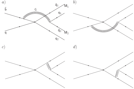
Figure 1: Feynman diagrams contributing to the amplitude of annihilation non-leptonic decay channels. The non-factorisable diagrams are a) and b), and the factorisable ones are c) and d).

III Annihilation Amplitudes

Annihilation decays are processes that occur at $\alpha_{s}$ order in perturbative QCD. A typical annihilation decay of a B meson is shown in Fig. 1, where the bottom quark decays through the W exchange or via a penguin process and a quark-antiquark pair is created in the final state through a gluon emission by any of the quarks involved in the process. The channels with these characteristics that we shall analyze are the following:

• Charmless channels :

  $\bar{B}^{0}_{s}\to\pi^{+}\pi^{-},\pi^{0}\pi^{0}$; $\bar{B}^{0}_{d}\to K^{+}K^{-}$;

• Charmed channels:

  $B^{0}\rightarrow D_{s}^{\pm(*)}K^{\mp}$; $B^{+}\rightarrow D_{s}^{+(*)}\bar{K}^{0}$;

  $B_{s}^{0}\rightarrow D^{\pm(*)}\pi^{\mp},D^{0}\pi^{0},\bar{D}^{0}\pi^{0}$.

In the following we present the analytical formulas for the computation of the amplitudes for the non-leptonic decays of B mesons.

III.1 Charmless channels

We present the amplitudes for the diagrams of Fig. 1, obtained with the help of Eq. (4). The diagrams that actually contribute for the amplitude of charmless decays are the non-factorisable diagrams shown in Figs. 1a and 1b, since the contributions from the factorisable ones (Figs. 1c and 1d) cancel among themselves. The full amplitude for the decays $\bar{B}\to\pi\pi,KK$ is given by

$${\mathcal{A}}(\bar{B}\to M_{1}M_{2}) = \frac{G_{F}}{\sqrt{2}}\,f_{B}f_{M_{1}}f_{M_{2}}(V_{ub}\,V_{uq}^{*}\,{\mathcal{A}}_{\mathrm{Tree}}$$ (12)

$$-V_{tb}\,V_{tq}^{*}\,{\mathcal{A}}_{\mathrm{Penguin}}),$$

with $q=d$ and $q=s$ for the decays of the $B_{d}^{0}$ and $B_{s}^{0}$ mesons, respectively. In particular the amplitude for the decay mode $\bar{B}_{s}^{0}\to\pi^{0}\pi^{0}$ relates to the one of the mode $\pi^{+}\pi^{-}$ as ${\mathcal{A}}(\bar{B}_{s}^{0}\to\pi^{0}\pi^{0})=\frac{1}{\sqrt{2}}{\mathcal{A}}(\bar{B}_{s}^{0}\to\pi^{+}\pi^{-})$.

We consider the $B$ meson at the rest frame, with momentum $P_{B}=\frac{m_{B}}{\sqrt{2}}(1,1,{\bf 0}_{T})$ in light-cone coordinates $(p^{+},$ $p^{-},{\bf p}_{T})$, with $p^{\pm}={1\over\sqrt{2}}(p^{0}\pm p^{3})$ and ${\bf p}_{T}=(p^{1},p^{2})$ (${\bf p}_{T}=\bf{0}_{T}$ in the collinear approximation). The mesons $M_{1}$ and $M_{2}$ have momenta defined as $P_{1}=\frac{m_{B}}{\sqrt{2}}(0,1,{\bf 0}_{T})\propto v$ and $P_{2}=\frac{m_{B}}{\sqrt{2}}(1,0,{\bf 0}_{T})\propto n$, hence $P_{B}=P_{1}+P_{2}$. We also define the momenta of the quarks in the mesons $B,M_{1},M_{2}$ respectively as $q=(zP_{B}^{+},0,{\bf 0}_{T})$, $q_{1}=(0,xP_{1}^{-},{\bf 0}_{T})$, $q_{2}=(yP_{2}^{+},0,{\bf 0}_{T})$ (the momentum of the antiquarks are given by $\bar{q}=P-q$).

The tree level and penguin amplitudes are

$${\mathcal{A}}_{\mathrm{Tree}}=C_{2}\,{\mathcal{A}}_{1}\,,$$ (13)

$${\mathcal{A}}_{\mathrm{Penguin}}=\left(2\,C_{4}+\frac{C_{10}}{2}\right)\,{\mathcal{A}}_{1}+\left(2\,C_{6}+\frac{C_{8}}{2}\right)\,{\mathcal{A}}_{2}.$$ (14)

The functions ${\mathcal{A}}_{1}$ and ${\mathcal{A}}_{2}$ are the contributions from operators of the type $(V-A)\otimes(V-A)$ and $(V-A)\otimes(V+A)$, respectively, and are given by

$${\mathcal{A}}_{1}=\frac{32\pi m_{B}^{4}C_{F}}{\sqrt{2N_{C}}}\int_{0}^{1}dx\,dy\,dz\,{\phi_{B}}(z)\biggl{\{}h_{b}(x,y,z)\times$$ (15)

$$\times \biggr{[}{-\bar{x}\phi_{A}}(x){\phi_{A}}(y)+\mu_{0P}^{2}\biggl{(}-4{\phi_{P}}(x){\phi_{P}}(y)+\left(\bar{z}-y\right)\times$$

$$\times ({\phi_{P}}(x)+{\phi_{T}}(x)({\phi_{P}}(y)-{\phi_{T}}(y))+x({\phi_{P}}(x)-{\phi_{T}}(x))\times$$

$$\times ({\phi_{P}}(y)+{\phi_{T}}(y))\biggr{)}\biggr{]}+h_{q}(x,y,z)\biggl{[}(y-z)\phi_{A}(x)\phi_{A}(y)+$$

$$+ \mu_{0P}^{2}\biggl{(}\bar{x}({\phi_{P}}(x)+{\phi_{T}}(x))({\phi_{P}}(y)-{\phi T}(y))+$$

$$+ (y-z)({\phi_{P}}(x)-{\phi_{T}}(x))({\phi_{P}}(y)+{\phi_{T}}(y))\biggr{)}\biggr{]}\biggr{\}},$$

and

$${\mathcal{A}}_{2}=\frac{32\pi m_{B}^{4}C_{F}}{\sqrt{2N_{C}}}\int_{0}^{1}dx\,dy\,dz\,{\phi_{B}}(z)\biggl{\{}h_{b}(x,y,z)\times$$ (16)

$$\times \biggl{[}\left(-y+\bar{z}-1\right){\phi_{A}}(x){\phi_{A}}(y)+\mu_{0P}^{2}\biggl{(}-4{\phi_{P}}(x){\phi_{P}}(y)+$$

$$+ x({\phi_{P}}(x)+{\phi_{T}}(x))({\phi_{P}}(y)-{\phi_{T}}(y))+\left(\bar{z}-y\right)({\phi_{P}}(x)+$$

$$- {\phi_{T}}(x))({\phi_{P}}(y)+{\phi_{T}}(y))\biggr{)}\biggr{]}+h_{q}(x,y,z)\biggl{[}\bar{x}{\phi_{A}}(x){\phi_{A}}(y)+$$

$$+{\mu_{0P}^{2}}\biggl{(}(y-z)({\phi)_{P}}(x)+{\phi_{T}}(x))({\phi_{P}}(y)-{\phi_{T}}(y))+$$

$$+\bar{x}({\phi_{P}}(x)-{\phi_{T}}(x))({\phi_{P}}(y)+{\phi_{T}}(y))\biggr{)}\biggr{]}\biggr{\}}.$$

Where $\mu_{0P}=m_{0P}/m_{B}$, and the functions $h(x,y,z)$ are

$$h_{b}(x,y,z) = \alpha(\mu)D_{b}(x,y,z)D_{g}(x,y)$$

$$h_{q}(x,y,z) = \alpha(\mu_{h})D_{q}(x,y,z)D_{g}(x,y),$$ (17)

and the quarks and gluon perturbative propagators are defined as:

$$D_{b}^{-1}(x,y,z) = m_{B}^{2}x(\bar{z}-y)-m_{b}^{2}$$

$$D_{q}^{-1}(x,y,z) = m_{B}^{2}\bar{x}(y-z)-m_{q}^{2}$$

$$D_{g}^{-1}(x,y) = (k_{g}^{2})^{-1}=m_{B}^{2}y\bar{x}$$ (18)

The scales adopted in the calculations are $\mu=m_{b}$ for the contribution from the diagram shown in Fig. 1a where the gluon is emitted from the $b$ quark, and $\mu_{h}=\sqrt{\Lambda_{h}m_{b}}$ for the contribution shown in Fig. 1b where the gluon is emitted from the spectator quark, with $\Lambda_{h}=500$ MeV beneke . When the effective scale is $\mu<m_{b}$ we use $\Lambda_{QCD}=225$ MeV and when $\mu=m_{b}$ we use $\Lambda_{QCD}=300$ MeV, and the difference is to match the values of the coupling constant due to different quark thresholds.

III.2 Charmed channels

The charmed decay channels occur through $W$ exchange processes, and there is no contribution from penguin diagrams. The full amplitude for the general processes $B\to D^{\mp}M^{\pm}$ (with $B=B_{d},B_{s}^{0},B^{+}$; $D,M={D_{(s)}^{\pm(*)},K,\pi}$) will be calculated from

$${\mathcal{A}}(B\to D^{-}M^{+}) = \frac{G_{F}}{\sqrt{2}}V_{uq}V_{cb}^{*}\,{\mathcal{M}}({B\to D^{-}M^{+}})\,,$$

$${\mathcal{A}}(B\to D^{+}M^{-}) = \frac{G_{F}}{\sqrt{2}}V_{cq}V_{ub}^{*}\,{\mathcal{M}}({B\to D^{+}M^{-}})\,,$$ (19)

where $q=d$ for the decays of $B^{0}$ and $B^{+}$, and $q=s$ for $B_{s}^{0}$.

We consider the $B$ meson at the rest frame, with momentum $P_{B}=\frac{m_{B}}{\sqrt{2}}(1,1,{\bf 0}_{T})$. The light mesons $M=\pi,K$ have momenta defined as $P_{M}=\frac{m_{B}}{\sqrt{2}}(0,1-r^{2},{\bf 0}_{T})\propto v$, and for the charmed mesons the momentum is $P_{D}=\frac{m_{B}}{\sqrt{2}}(1,r^{2},{\bf 0}_{T})$, hence $P_{B}=P_{M}+P_{D}$. The momentum of the quarks are defined analogously to the charmless case.

The functions ${\mathcal{M}}$ in the previous Eqs. (19) are the sum of factorisable and non-factorisable contributions, ${\mathcal{M}}={\mathcal{M}}_{\mathrm{fac}}+{\mathcal{M}}_{\mathrm{nfac}}$. The analytical formulas for these contributions for the decays with two pseudo-scalar particles in the final state, are the following:

• ${B^{0}\to D^{-}M^{+}}$:

$${\mathcal{M}}_{\mathrm{fac}}({{B^{0}\to D^{-}M^{+}}})=\frac{8\pi m_{B}^{4}C_{F}}{\sqrt{2N_{C}}}\int_{0}^{1}{dx}\,{dy}\,{dz}$$ (20)

$$\times \phi_{B}(z)\phi_{D}(y)\biggr{\{}-\biggr{(}(1-r^{2})y\phi_{A}(x)-2r\mu_{0P}(1-r^{2}+y)\phi_{P}(x)\biggl{)}\times$$

$$\times h_{l}(x,y,z)-\biggr{(}(1-r^{2})(r^{2}-(1-r^{2})\bar{x})\phi_{A}(x)-r\mu_{0P}(3-r^{2}+$$

$$- 2(1-r^{2})x)\phi_{P}(x)-(1-r^{2})(1-2x)\phi_{T}(x)\biggl{)}h_{c}(x,y,z)\biggl{\}}\,,$$

$${\mathcal{M}}_{\mathrm{nfac}}({{B^{0}\to D^{-}M^{+}}})=\frac{32\pi m_{B}^{4}C_{F}}{\sqrt{2N_{C}}}\int_{0}^{1}{dx}\,{dy}\,{dz}\phi_{B}(z)\phi_{D}(y)\times$$ (21)

$$\times \biggr{\{}-\biggr{(}(1-r^{2})((1+r^{2})(y-\bar{z})-1)\phi_{A}(x)-r\mu_{0P}\bigr{(}(2+y+z+$$

$$+ (1-r^{2})\bar{x})\phi_{P}(x)+(-y+z+(1-r^{2})\bar{x})\phi_{T}(x)\bigl{)}\biggl{)}h_{b}(x,y,z)+$$

$$+ \biggr{(}(1-r^{2})((y-z)r^{2}+(1-r^{2})\bar{x})\phi_{A}(x)+r\mu_{0P}\bigr{(}(y-z+$$

$$+ (1-r^{2})\bar{x})\phi_{P}(x)+(y-z-(1-r^{2})\bar{x})\phi_{T}(x)\bigl{)}\biggl{)}h_{q}(x,y,z)\biggl{\}}\,.$$

• ${B^{0}\to D^{+}M^{-}}$:

$${\mathcal{M}}_{\mathrm{fac}}({{B^{0}\to D^{+}M^{-}}})=-{\mathcal{M}}_{fac}({{B^{0}\to D^{-}M^{+}}})$$ (22)

$${\mathcal{M}}_{\mathrm{nfac}}({{B^{0}\to D^{+}M^{-}}})=\frac{32\pi m_{B}^{4}C_{F}}{\sqrt{2N_{C}}}\int_{0}^{1}{dx}\,{dy}\,{dz}\times$$ (23)

$$\times \phi_{B}(z)\phi_{D}(y)\biggr{\{}-\biggr{(}(1-r^{2})((1-r^{2})\bar{x}+(y-\bar{z})r^{2})\phi_{A}(x)+$$

$$- r\mu_{0P}\bigr{(}(2+y+z+(1-r^{2})\bar{x})\phi_{P}(x)+((1-r^{2})\bar{x}+$$

$$+ y+z)\phi_{T}(x)\bigl{)}\biggl{)}h_{b}(x,y,z)+\biggr{(}(1-r^{4})(y-z)\phi_{A}(x)+$$

$$+ r\mu_{0P}\bigr{(}(y-z+(1-r^{2})\bar{x})\phi_{P}(x)+$$

$$+ (-y+z+(1-r^{2})\bar{x})\phi_{T}(x)\bigl{)}\biggl{)}h_{q}(x,y,z)\biggl{\}}$$

For decays with one vector plus one pseudo-scalar particles in the final state, the analytical formulas are the following:

• ${B^{0}\to D^{*-}M^{+}}$:

$${\mathcal{M}}_{\mathrm{fac}}({{B^{0}\to D^{*-}M^{+}}})=\frac{8\pi m_{B}^{4}C_{F}}{\sqrt{2N_{C}}}\int_{0}^{1}{dx}\,{dy}\,{dz}\phi_{B}(z)\times$$ (24)

$$\times \phi_{D}(y)\biggr{\{}\biggr{(}(1-r^{2})y\phi_{A}(x)-2r\mu_{0P}(1-r^{2}-yy)\phi_{P}(x)\biggl{)}\times$$

$$\times h_{l}(x,y,z)-\biggr{(}(1-r^{2})(1-(1-r^{2})x)\phi_{A}(x)+$$

$$+ r\mu_{0P}((1-r^{2}))\phi_{P}(x)-(1+r^{2})\phi_{T}(x)\biggl{)}h_{c}(x,y,z)\biggl{\}}$$

$${\mathcal{M}}_{{\mathrm{nfac}}}({{B^{0}\to D^{*-}M^{+}}})=\frac{32\pi m_{B}^{4}C_{F}}{\sqrt{2N_{C}}}\int_{0}^{1}{dx}\,{dy}\,{dz}\,\times$$ (25)

$$\times \phi_{B}(z)\phi_{D}(y)\biggr{\{}-\biggr{(}(1-r^{2})((1-r^{2})(y+z)+r^{2})\phi_{A}(x)+$$

$$-r\mu_{0P}\bigr{(}(y+z-(1-r^{2})\bar{x})\phi_{P}(x)+(y+z-2r^{2}+$$

$$- (1-r^{2})(1+x))\phi_{T}(x)\bigl{)}\biggl{)}h_{b}(x,y,z)+$$

$$+ \biggr{(}(1-r^{2})((1-r^{2})-r^{2}(y-z)\bar{x})\phi_{A}(x)+$$

$$- r\mu_{0P}\bigr{(}(y-z-(1-r^{2})\bar{x})\phi_{P}(x)+$$

$$+ (y-z+(1-r^{2})\bar{x})\phi_{T}(x)\bigl{)}\biggl{)}h_{q}(x,y,z)\biggl{\}}$$

• ${B^{0}\to D^{*+}M^{-}}$:

$${\mathcal{M}}_{\mathrm{fac}}({{B^{0}\to D^{*+}M^{-}}})=-{\mathcal{M}}_{fac}({{B^{0}\to D^{*-}M^{+}}})$$ (26)

$${\mathcal{M}}_{\mathrm{nfac}}({{B^{0}\to D^{*+}M^{-}}})=\frac{32\pi m_{B}^{4}C_{F}}{\sqrt{2N_{C}}}\int_{0}^{1}{dx}\,{dy}\,{dz}\times$$

$$\times\phi_{B}(z)\,\phi_{D}(y)\,\biggr{\{}-\biggr{(}(1-r^{2})(1-(y+z)r^{2}-(1-r^{2})x)\times$$

$$\times\phi_{A}(x)+r\mu_{0P}\bigr{(}(y+z-(1-r^{2})\bar{x})\phi_{P}(x)-(y+z+$$

$$-2r^{2}-(1-r^{2})(1+x))\phi_{T}(x)\bigl{)}\biggl{)}h_{b}(x,y,z)+$$

$$+\biggr{(}(1-2r^{2})(y-z)\bar{x})\phi_{A}(x)+r\mu_{0P}\bigr{(}(y-z-(1-r^{2})\bar{x})\times$$

$$\times\phi_{P}(x)-(y-z+(1-r^{2})\bar{x})\phi_{T}(x)\bigl{)}\biggl{)}h_{q}(x,y,z)\biggl{\}}$$ (27)

In the charged decay modes $B^{+}\to D_{s}^{(*)+}\bar{K}^{0}$ the analytical formulas for the amplitudes are easily obtained from the ones of the neutral modes $B^{0}\to D_{s}^{(*)+}K^{-}$, given in Eqs. (20),(21),(24) and (25). The simpler way to see this, is that the operators that contributes to the neutral decay modes are related to the ones that contributes to the charged modes by replacing the spectator quark of the $B$ meson $d\to u$ (i.e., $\bar{b}d\to\bar{b}u$), and the light quark from the $K$ meson is also replaced $u\to d$ (i.e., $\bar{u}s\to\bar{d}s$). The final result in the calculation of the amplitudes of the charged modes are equivalent to the neutral mode, with the replacement of the distribution, $\phi_{B^{0}}\to\phi_{B^{+}}$ and $\phi_{K}\to\phi_{K^{0}}$. Also the analytical expression of the distribution amplitudes are equivalent, with the use of the respective mass and decay constant of each meson. Besides that, the amplitudes of decay modes which involves two neutral pseudoscalar mesons in the final states are related to the modes of charged pseudoscalars as

$${\mathcal{A}}(B\to M_{1}^{0}M_{2}^{0})=\frac{1}{\sqrt{2}}{\mathcal{A}}(B\to M_{1}^{+}M_{2}^{-})$$

In Eqs. (20) to (III.2) we define the following functions:

$$h_{c}(x,y,z)=D_{c}(x)\,D_{g}(x,y)\alpha_{s}(\mu_{f})\bigl{(}C_{1}(\mu_{f})+{C_{2}(\mu_{f})}/{3}\bigr{)}\,;$$

$$h_{l}(x,y,z)=D_{l}(x)D_{g}(x,y)\alpha_{s}(\mu_{f})\bigl{(}C_{1}(\mu_{f})+C_{2}(\mu_{f})/3\bigr{)}\,;$$

$$h_{q}(x,y,z)=D_{q}(x)D_{g}(x,y)\alpha_{s}(\mu_{h})C_{2}(\mu_{h})\,;$$

$$h_{b}(x,y,z)=D_{b}(x)D_{g}(x,y)\alpha_{s}(\mu)C_{2}(\mu)\,,$$ (28)

where the functions $D_{b}(x,y,z),\,D_{d}(x,y,z),\,D_{u}(y)$ and $D_{c}=D_{c}(x)$ and $D_{g}(x,y)$ are the quarks and gluon propagators, given by:

$$D_{b}^{-1}(x,y,z) = m_{B}^{2}((y-\bar{z})(1-\bar{x}(1-r^{2})))-m_{b}^{2};$$

$$D_{q}^{-1}(x,y,z) = m_{B}^{2}\bar{x}(z-y)(1-r^{2});$$

$$D_{c}^{-1}(x) = m_{B}^{2}(r^{2}+\bar{x}(1-r^{2}))-m_{c}^{2}\,;$$

$$D_{l}^{-1}(y) = m_{B}^{2}y(1-r^{2})\,$$

$$D_{g}^{-1}(x,y) = k_{g}^{2}=m_{B}^{2}y\,(1-x)\,(1-r^{2}).$$ (29)

For the charged modes, the Wilson coefficients that appear in Eqs. (28) are exchanged by $C_{1}(\mu_{f})/3+{C_{2}(\mu_{f})}$ for the first two lines, and by $C_{1}(\mu)$ for the last two lines.

Note that the perturbative propagators are going to be substituted by the non-perturbative ones discussed in the next section. The scales adopted in the calculations are the same as the charmless case: $\mu=m_{b}$ for the contribution of the diagram where the gluon is emitted from the $b$ quark, and $\mu_{h}=\sqrt{\Lambda_{h}m_{b}}$ for the contribution where the gluon is emitted from the “spectator” quark, with $\Lambda_{h}=500$ MeV. For the diagrams of Fig. 1c and 1d where the gluon is emitted from the quarks in the final state, we use the scale $\mu_{f}=\mu/2=m_{b}/2$. The QCD scales are also the same as the charmless case.

IV Regulation of the divergences

The annihilation amplitudes have both soft and collinear divergences. The soft divergences occur with the vanishing of the gluon momentum, and this one has been treated with an ad hoc cutoff as shown in Eq.(1). In our work this procedure is exchanged by the introduction of an IR finite gluon propagator obtained through the solution of Schwinger-Dyson equations (SDE) cornwall ; bp ; ap ; an2 ; cornwall2 and consistent with recent lattice data abp . As for the collinear divergences, we can include the dynamical mass of the light quarks, which are also necessary to keep the consistency with the introduction of dynamical gluon masses. The poles of the (massive) propagators will give the imaginary part of the amplitudes. Therefore, the basic point in the regulation of divergences is based on the use of non-perturbative IR information (or dressed propagators) in the context of the perturbative expansion. We will discuss this regulation scheme in detail in the following.

IV.1 IR finite gluon propagator

A prescription of how non-perturbative SDE solutions can be inserted into the perturbative QCD expansion was proposed by Pagels and Stokar many years ago, in the approach denominated dynamical perturbation theory (DPT) pagels . In their scheme the amplitudes that do not vanish to all orders in perturbation theory are given by their free field values, while amplitudes that vanish as $\lambda\propto e^{-1/g^{2}}$ are retained, and possibly dealt with in an expansion in $g^{n}\lambda$. The work of Ref.pagels was particularly concerned with the effect of a dynamically generated quark mass, but from SDE cornwall ; bp ; ap ; an2 ; cornwall2 and lattice simulations abp we now know that the gluon and coupling constant also have an infrared finite value, and the Pagels and Stokar formulation can be extended and generalized for the perturbative expansion using the quark and gluon propagators with a dynamical mass and the IR finite coupling constant. Actually we expect that any infrared finite gluon propagator leads to a freezing of the infrared coupling constant natale2 , meaning that the use of an infrared finite gluon propagator must be accompanied by an IR finite coupling constant. All these facts indicate that we should perform perturbation theory with the dressed quark and gluon propagators and the effective charge (dependent on the gluon mass).

The SDE solution and the lattice result that we shall use were discussed at length in the following references abp ; trento , therefore we will not enter into further details about the solutions and will just present the gluon propagator and coupling constant in the case that QCD generates a dynamical gluon mass. We consider a gluon propagator that will have the form

$$\imath{{\Delta}}_{\mu\nu}(q)=P_{\mu\nu}{\Delta}(q)+\xi\frac{q_{\mu}q_{\nu}}{q^{4}}\,\,;\,\,P_{\mu\nu}=-g_{\mu\nu}+\frac{q_{\mu}q_{\nu}}{q^{2}}\,\,,$$ (30)

where ${\Delta}(q)$ is the gauge invariant scalar part of the gluon propagator, which in Euclidean space has the form

$${\Delta}(Q^{2})\propto\frac{1}{Q^{2}+m_{g}^{2}(Q^{2})}\,\,.$$ (31)

The gluonic SDE solutions allow us to write a new propagator ${\hat{\Delta}}^{-1}(Q^{2})$ which absorbs all the renormalization group logs, exactly as happens in QED with the photon self-energy, and form the product ${\hat{d}}(Q^{2})=g^{2}{\hat{\Delta}}(Q^{2})$ which is a renormalization group invariant. The dynamical gluon mass ($m_{g}^{2}(Q^{2})$) cornwall is given by

$$m_{g}^{2}(Q^{2})=m_{g}^{2}\left[\frac{\mathrm{ln}\left(\frac{q^{2}+4m_{g}^{2}}{\Lambda^{2}}\right)}{\mathrm{ln}\left(\frac{4m_{g}^{2}}{\Lambda^{2}}\right)}\right]^{-\frac{12}{11}},$$ (32)

where the gluon mass scale $m_{g}$ has typical values cornwall ; several

$$m_{g}=500\pm 200\,\mathrm{MeV}\,\,\,.$$ (33)

As this is a complicated expression to take into account when performing the numerical integration, in practical calculations, the best we can do is to assume $m_{g}^{2}(Q^{2})\approx m_{g}^{2}$. In this work the dynamical gluon mass is calculated at the same scales described in the end of the Section III. There is no significant difference in the results if we neglect the running of the masses, since slightly away from the mass value the effect of momentum dependence takes over the full propagator effect”.

A simple fit for the coupling constant that is factored out in this procedure is given by cornwall

$${\bar{\alpha}}_{sd}(q^{2})=\frac{1}{4\pi b\ln[(4m_{g}^{2}-q^{2}-\imath\epsilon)/\Lambda^{2}]}\,\,,$$ (34)

where $b=(33-2n_{f})/48\pi^{2}$. Eq.(34) clearly shows the existence of the IR fixed-point as $q^{2}\rightarrow 0$. It must be stressed that the fixed point does not depend on a specific process, it is uniquely obtained as we fix $\Lambda$ and, in principle, it should be exactly determined if we knew how to solve QCD. Several examples of the use of DPT with the propagator and coupling constant discussed above can be found in Ref.several .

IV.2 Dynamical quark masses

The dressed quark propagator can be written as

$$S(p)=\frac{Z(p^{2})}{\imath\gamma\cdot p+M(p^{2})}\,\,,$$ (35)

where $Z(p^{2})$ is the Lorentz scalar quark wave function renormalization and $M(p^{2})$ is the quark dynamical mass. At large momenta, and in the chiral limit, it is known that that the dynamical mass is related to the quark condensate ($<{\bar{q}}q>$) as rob

$$M(p^{2})\propto\frac{<{\bar{q}}q>}{p^{2}}\,\,.$$ (36)

The many estimates of the dynamical quark mass ($M(0)$) (among them we have $M(0)\propto<{\bar{q}}q>^{1/3}$) give values between $250\mbox{ MeV}$ and $300\mbox{ MeV}$ rob ; maris , whereas we can safely assume $Z(p^{2})\approx 1$. The decrease of the mass with the momentum shown in Eq.(36) is not going to be considered, since the mass function has a plateau at low momenta and decreases (in the chiral limit) very fast at high momenta maris , where the propagator is dominated by the $\imath\gamma\cdot p$ term, in such a way that our calculation is not affected if we take the quark propagator as $S(p)={1}/({\imath\gamma\cdot p+M(0))}$.

V Numerical Results

We perform the numerical calculation considering the gluon mass scale with values $m_{g}=400\mbox{ MeV},500\mbox{ MeV}$. The dynamical masses of the light quarks are $M(0)=m_{u}=m_{d}$, in the interval $250\mbox{ MeV}<M(0)<300\mbox{ MeV}$, and the same value is assumed for the $s$ quark, although it has been argued that the constituent $s$ quark mass may be slightly higher maris . For the the light mesons, pions and kaons, we use the asymptotic expression for the wave functions

$$\phi^{A}(x)\,=\frac{f_{P}}{2\sqrt{2N_{C}}}6\,x\,(1-x),\qquad\phi^{P}(x)=\frac{f_{P}}{2\sqrt{2N_{C}}}$$

$$\phi^{T}(x)=\frac{f_{P}}{2\sqrt{2N_{C}}}(2x-1)$$ (37)

while for the $D(D^{*})$ mesons we use

$$\Phi_{D}(x)\,=\frac{f_{D}}{2\sqrt{2N_{C}}}6\,x\,(1-x)\,[1+a_{D}(1-2x)],$$ (38)

with $a_{D}=0.8$ for $D$ and $a_{D}=0.3$ for $D_{s}$ mesons Lu:2002iv ; Li:2005vu . The momentum of the $B$ meson is carried almost all by the $b$ quark, and the light quark carries a momentum of the order $\Lambda_{QCD}$. Providing that we assume $z\sim\Lambda_{QCD}/m_{b}$ and $x,y\gg z$, at leading order the integration over the $B$ meson wave function is trivial, yielding to the decay constant according to the Eq. (8). This procedure has been adopted in annihilation decay calculations by Beneke et. al beneke .

The Wilson’s coefficients are computed using the equations given in the appendices of Ref. Lu:2000em . We also use the following parameters Amsler:2008zzb :

• Masses:

  $m_{B}=5.28$ GeV, $m_{B_{s}}=5.37$ GeV, $m_{D}=1.87$ GeV, $m_{D_{s}}=1.97$ GeV, $m_{D^{*}}=2.01$ GeV, $m_{D_{s}^{*}}=2.10$ GeV, $m_{b}=4.7$ GeV. $m_{c}=1.27$ GeV.

• Lifetimes:

  $\tau_{B_{d}}=1.54$ ps, $\tau_{B_{s}}=1.466$ ps, $\tau_{B^{+}}=1.638$ ps .

• CKM parameters:

  $A=0.814$, $\lambda=0.2257$, $\bar{\rho}=0.135$, $\bar{\eta}=0.349$.

• Decay constants stone ; fdlattice :

  $f_{B}=190\mbox{ MeV}$, $f_{B_{s}}=236\mbox{ MeV}$ ; $f_{D}=206\mbox{ MeV}$, $f_{D_{s}}=257\mbox{ MeV}$, $f_{\pi}=130\mbox{ MeV}$, $f_{K}=156\mbox{ MeV}$; $f_{D^{*}}=245\mbox{ MeV}$, $f_{D_{s}^{*}}=272\mbox{ MeV}$.

In Table 1 we show the results obtained and the experimental data available for each decay channel.

Table 1: Branching ratios for $B$ decays. The error correspond to the variation of the dynamical quark mass, $250\mbox{ MeV}<m_{q}<300\mbox{ MeV}$. We show the results for the gluon mass scale $m_{g}=400\mbox{ MeV}$ and $500\mbox{ MeV}$. In the last column are shown the available experimental data.

Channel	$m_{g}=400\mbox{ MeV}$	$m_{g}=500\mbox{ MeV}$	Experimental Data Amsler:2008zzb
$\bar{B}^{0}\to K^{+}K^{-}$	$(4.31\pm 0.50)\times 10^{-8}$	$(3.20\pm 0.01)\times 10^{-8}$	$<4.1\times 10^{-7}$
$\bar{B}_{s}^{0}\to\pi^{+}\pi^{-}$	$(10.42\pm 1.00)\times 10^{-7}$	$(5.32\pm 0.25)\times 10^{-7}$	$<1.7\times 10^{-6}$
$\bar{B}_{s}^{0}\to\pi^{0}\pi^{0}$	$(5.21\pm 0.05)\times 10^{-7}$	$(2.66\pm 0.13)\times 10^{-7}$	$<2.1\times 10^{-6}$
$B^{0}\to D_{s}^{-}K^{+}$	$(6.12\pm 0.78)\times 10^{-5}$	$(3.07\pm 0.17)\times 10^{-5}$	$2.9\pm 0.5$
$B^{0}\to D_{s}^{+}K^{-}$	$(6.15\pm 0.71)\times 10^{-8}$	$(2.92\pm 0.23)\times 10^{-8}$
$B^{+}\to D_{s}^{+}\bar{K^{0}}$	$(0.89\pm 0.16)\times 10^{-8}$	$(0.32\pm 0.11)\times 10^{-8}$	$<9\times 10^{-4}$
$B_{s}^{0}\to D^{-}\pi^{+}$	$(1.72\pm 0.04)\times 10^{-6}$	$(1.18\pm 0.40)\times 10^{-6}$
$B_{s}^{0}\to\bar{D}^{0}\pi^{0}$	$(0.86\pm 0.02)\times 10^{-6}$	$(0.61\pm 0.17)\times 10^{-6}$
$B_{s}^{0}\to D^{+}\pi^{-}$	$(5.80\pm 0.60)\times 10^{-7}$	$(2.51\pm 0.96)\times 10^{-7}$
$B_{s}^{0}\to D^{0}\pi^{0}$	$(2.90\pm 0.30)\times 10^{-7}$	$(1.26\pm 0.48)\times 10^{-7}$
$B^{0}\to D_{s}^{*-}K^{+}$	$(2.85\pm 0.18)\times 10^{-5}$	$(1.90\pm 0.06)\times 10^{-5}$	$2.2\pm 0.6$
$B^{0}\to D_{s}^{*+}K^{-}$	$(6.23\pm 0.50)\times 10^{-8}$	$(2.68\pm 0.07)\times 10^{-8}$
$B^{+}\to D_{s}^{*+}\bar{K^{0}}$	$(1.71\pm 0.52)\times 10^{-8}$	$(1.28\pm 0.22)\times 10^{-8}$	$<9\times 10^{-4}$
$B_{s}^{0}\to D^{*-}\pi^{+}$	$(3.36\pm 0.06)\times 10^{-6}$	$(1.88\pm 0.21)\times 10^{-6}$
$B_{s}^{0}\to D^{*+}\pi^{-}$	$(3.26\pm 0.29)\times 10^{-8}$	$(3.92\pm 1.31)\times 10^{-8}$

VI Conclusion

We have studied some decay channels of $B^{0}_{s},\,B^{0}_{d},\,B^{+}$ mesons which occur through the annihilation diagrams. We have argued that infrared finite gluon propagators and running coupling constants obtained as solutions of the QCD Schwinger-Dyson equations, may serve as a natural cutoff for the end-point divergences that appear in the calculation of these decays. Also, we use the constituent quark mass for the light quarks in the propagators to be able to perform the twist-3 calculation of the amplitudes.

Comparing to the data available, our calculations are very satisfactory, notably for the two channels with actual measurements $B^{0}\to D_{s}^{-}K^{+}$ and $B^{0}\to D_{s}^{-*}{K}^{+}$. The results are also reasonably compatible with some predictions of the pQCD in the $k_{T}$ factorization, see for example Refs. Chen:2000ih ; Lu:2002iv ; Li:2003wg ; Li:2005vu ; Ali:2007ff ; Li:2008ts ; Zou:2009zza .

We can see from the results that the variation on the dynamical mass of the quarks generally introduces only a small error. The numerical results are more dependent on the gluon mass scale, as we can see a more significant variation of the results with this mass scale. Comparing to the available data it is possible to narrow the interval for the gluon mass scale for values closer to $m_{g}=500\mbox{ MeV}$. This value for the gluon mass scale is in accordance with previous calculations several . Future measurements for the other decay modes, besides $B^{0}\to D_{s}^{-}K^{+}$ and $B^{0}\to D_{s}^{-*}{K}^{+}$, can establish a more precise value for the $m_{g}$ parameter. Besides the annihilation modes, it is also possible to apply the present regulation prescriptions to other types of $B$ decay.

The already existent agreement of some B decays with the experimental data and the possible future confirmation of the other rare decays computed here, may indicate that the introduction of the nonperturbative information provided by the Schwinger-Dyson equations in the form of dynamical masses for quarks and gluons, consistent with the most recent lattice QCD simulations, is gathering more and more robust phenomenological results showing that these mass scales possibly cannot be neglected when performing high precision hadronic calculations.

VII Acknowledgments

This research was supported by the FAPESP (CMZ) and CNPq (AAN).

References

• (1) G. P. Lepage and S. J. Brodsky, Phys. Lett. B87, 359 (1979).
• (2) G. P. Lepage and S. J. Brodsky, Phys. Rev. D 22, 2157 (1980).
• (3) A. Szczepaniak, E. M. Henley, and S. J. Brodsky, Phys. Lett. B243, 287 (1990).
• (4) H. N. Li and H. L. Yu, Phys. Rev. Lett. 74, 4388 (1995a), eprint hep-ph/9409313.
• (5) H. N. Li and H. L. Yu, Phys. Lett. B353, 301 (1995b).
• (6) H. N. Li, Phys. Rev. D52, 3958 (1995), eprint hep-ph/9412340.
• (7) C. D. Lu, K. Ukai and M. Z. Yang, Phys. Rev.  D 63, 074009 (2001) [arXiv:hep-ph/0004213].
• (8) Y. Y. Keum, H. N. Li, and A. I. Sanda, Phys. Rev. D63, 054008 (2001), eprint hep-ph/0004173.
• (9) M. Beneke, G. Buchalla, M. Neubert, and C. T. Sachrajda, Phys. Rev. Lett. 83, 1914 (1999), eprint hep-ph/9905312.
• (10) M. Beneke, G. Buchalla, M. Neubert, and C. T. Sachrajda, Nucl. Phys. B591, 313 (2000), eprint hep-ph/0006124.
• (11) M. Beneke, G. Buchalla, M. Neubert, and C. T. Sachrajda, Nucl. Phys. B606, 245 (2001), eprint hep-ph/0104110.
• (12) M. Beneke and M. Neubert, Nucl. Phys. B675, 333 (2003), eprint hep-ph/0308039.
• (13) S. Bar-Shalom, G. Eilam, and Y. D. Yang, Phys. Rev. D67, 014007 (2003), eprint hep-ph/0201244.
• (14) Y. D. Yang, F. Su, G. R. Lu, and H. J. Hao, Eur. Phys. J. C44, 243 (2005), eprint hep-ph/0507326.
• (15) Y. L. W. F. Su, Y. D. Yang, and C. Zhuang, Eur. Phys. J. C48, 401 (2006), eprint hep-ph/0604082.
• (16) A. A. Natale, C. M. Zanetti, Int. J. Mod. Phys., A24, 2009, 4133.
• (17) Q. Chang, X. Q. Li, Y. D. Yang, JHEP,09, 038, 2008.
• (18) Q. Chang, X. Q. Li and Y. D. Yang, JHEP 0905, 056 (2009) [arXiv:0903.0275 [hep-ph]].
• (19) J. M. Cornwall, Phys. Rev. D 26, 1453 (1982); hep-ph/0904.3758.
• (20) A. C. Aguilar, D. Binosi and J. Papavassiliou, Phys. Rev. D 78, 025010 (2008); for a quite recent lattice calculation containing earlier references see D. Dudal, O. Oliveira and N. Vandersickel, eprint hep-lat/1002.2374.
• (21) G. Buchalla, A. J. Buras, and M. E. Lautenbacher, Rev. Mod. Phys. 68, 1125 (1996), eprint hep-ph/9512380.
• (22) C. D. Lu and M. Z. Yang, Eur. Phys. J.  C 28, 515 (2003) [arXiv:hep-ph/0212373].
• (23) T. Kurimoto, H. n. Li and A. I. Sanda, Phys. Rev.  D 67, 054028 (2003) [arXiv:hep-ph/0210289].
• (24) D. Binosi and J. Papavassiliou, Phys. Rept. 479, 1 (2009).
• (25) A. C. Aguilar and J. Papavassiliou, Eur. Phys. J. A 35, 189 (2008).
• (26) A. C. Aguilar and A. A. Natale, JHEP 0408, 057 (2004).
• (27) J. M. Cornwall, hep-ph/0904.3758.
• (28) H. Pagels and S. Stokar, Phys. Rev. D 20, 2947 (1979).
• (29) A. C. Aguilar, A. A. Natale and P. S. Rodrigues da Silva, Phys. Rev. Lett. 86 (2003) 152001.
• (30) A list of references on SDE solutions and lattice results about the infrared finite gluon propagator can be found in the second paper of Ref.cornwall , as well as in the Proceedings of the International Workshop on QCD Green s Functions, Confinement and Phenomenology, September 7-11, 2009 ECT, Trento, Italy, (PoS QCD-TNT 09 (2009)), in particular, see A. A. Natale, hep-ph/0910.5689; A. C. Aguilar, hep-ph/0911.4372; J. Papavassiliou, hep-ph/0911.3912; D. Binosi, hep-ph/0911.0315.
• (31) H. Chehime et al., Phys. Lett. B 286, 397 (1992); F. Halzen, G. I. Krein and A. A. Natale, Phys. Rev. D 47, 295 (1993); M. B. Gay Ducati, F. Halzen and A. A. Natale,Phys. Rev. D 48, 2324 (1993); A. Mihara and A. A. Natale, Phys. Lett. B 482, 378 (2000); A. C. Aguilar, A. Mihara and A. A. Natale, Phys. Rev. D 65, 054011 (2002); E. G. S. Luna, A. F. Martini, M. J. Menon, A. Mihara and A. A. Natale, Phys. Rev. D 72, 034019 (2005); E. G. S. Luna and A. A. Natale, Phys. Rev. D 73, 074019 (2006); E. G. S. Luna, Phys. Lett. B. 641, 171 (2006); F. Carvalho, A. A. Natale and C. M. Zanetti, Mod. Phys. Lett. A 21, 3021 (2006); A. A. Natale, Braz. J. Phys. 37, 306 (2007); E. G. S. Luna, A. A. Natale and C. M. Zanetti, Int. J. Mod. Phys. A 2, 151 (2008).
• (32) C. D. Roberts and A. G. Williams, Prog. Part. Nucl. Phys. 33, 477 (1994); C. D. Roberts, Prog. Part. Nucl. Phys. 61, 50 (2008).
• (33) P. Maris and C. D. Roberts, Contribution to the IVth International Workshop on Progress in Heavy Quark Physics, 20-22 Sept. 1997, Rostock, nucl-th/9710062.
• (34) J. N. Rosner and S. Stone, arXiv: 1002.1655 [hep-ex]
• (35) D. Becirevic et al., Phys. Rev. D 60, 074501 (1999).
• (36) C. Amsler et al. [Particle Data Group], Phys. Lett.  B 667, 1 (2008).
• (37) C. H. Chen and H. n. Li, Phys. Rev.  D 63, 014003 (2000) [arXiv:hep-ph/0006351].
• (38) C. D. Lu and K. Ukai, Eur. Phys. J.  C 28, 305 (2003) [arXiv:hep-ph/0210206].
• (39) Y. Li and C. D. Lu, J. Phys. G 29, 2115 (2003) [arXiv:hep-ph/0304288].
• (40) Y. Li and C. D. Lu, Commun. Theor. Phys.  44, 659 (2005) [arXiv:hep-ph/0502038].
• (41) A. Ali, G. Kramer, Y. Li, C. D. Lu, Y. L. Shen, W. Wang and Y. M. Wang, Phys. Rev.  D 76, 074018 (2007) [arXiv:hep-ph/0703162].
• (42) R. H. Li, C. D. Lu and H. Zou, Phys. Rev.  D 78, 014018 (2008) [arXiv:0803.1073 [hep-ph]].
• (43) H. Zou, R. H. Li, X. X. Wang and C. D. Lu, J. Phys. G 37, 015002 (2010) [arXiv:0908.1856 [hep-ph]].