A parametric physical model for the intracluster medium and its use in joint SZ/X-ray analyses of galaxy clusters

Abstract

We present a parameterized model of the intra-cluster medium that is suitable for jointly analysing pointed observations of the Sunyaev-Zel’dovich (SZ) effect and X-ray emission in galaxy clusters. The model is based on assumptions of hydrostatic equilibrium, the Navarro, Frenk and White (NFW) model for the dark matter, and a softened power law profile for the gas entropy. We test this entropy-based model against high and low signal-to-noise mock observations of a relaxed and recently-merged cluster from $N$-body/hydrodynamic simulations, using Bayesian hyper-parameters to optimise the relative statistical weighting of the mock SZ and X-ray data. We find that it accurately reproduces both the global values of the cluster temperature, total mass and gas mass fraction ($f_{\mathrm{gas}}$), as well as the radial dependencies of these quantities outside of the core ($r>100\,\mathrm{kpc}$). For reference we also provide a comparison with results from the single isothermal $\beta$ model. We confirm previous results that the single isothermal $\beta$ model can result in significant biases in derived cluster properties.

1 Introduction

The Sunyaev-Zel’dovich effect is a distortion of the Cosmic Microwave Background (CMB) spectrum by inverse Compton scattering off a hot population of electrons, such as in the intra-cluster medium (ICM) of a galaxy cluster (Sunyaev & Zel’dovich, 1970; Birkinshaw, 1999). The SZ effect is observable as an anisotropy in the CMB and has a surface brightness that is proportional to the line-of-sight integral of the gas pressure of the cluster, independent of redshift. Since the surface brightness is independent of redshift, SZ observations provide a powerful tool to probe the properties of the largest virialised structures in the Universe. Over the past decade there has been considerable observational data gathered on the ICM properties of clusters via the SZ effect (e.g. Grego et al., 2001; LaRoque et al., 2006) and we are now entering an era of deep cluster surveys with specifically designed SZ telescopes, including the South Pole Telescope (SPT, Ruhl et al., 2004), the Sunyaev-Zel’dovich Array (SZA, Muchovej et al., 2007), the Atacama Cosmology Telescope (ACT, Kosowsky, 2003) and the Arcminute Microkelvin Imager (AMI, Zwart et al., 2008). These surveys will make use of the redshift independence of the SZ surface brightness to map the distribution and evolution of large scale structure throughout the Universe.

In order to interpret the data from SZ surveys we require well-calibrated scaling relations between the SZ signal and physical properties and a good physical understanding of the intrinsic scatter therein. Pointed SZ observations with interferometer and bolometer arrays coupled with X-ray imaging and spectra allow us to probe the intra-cluster medium, while weak and strong gravitational lensing observations directly measure the projected gravitational potential and hence total mass of the cluster. Recently, there has been concerted effort in developing physically motivated analytic models that account for the observed non-isothermality in cluster gas [see e.g. Komatsu & Seljak 2001; Ostriker et al. 2005; Atrio-Barandela et al. 2008; Bulbul et al. 2010 (polytropic equation of state), Pointecouteau et al. 2004; Vikhlinin et al. 2006; Mahdavi et al. 2007 (component separation and modified $\beta$ models), and Nagai et al. 2007; Mroczkowski et al. 2009; Arnaud et al. 2010 (explicit pressure parametrization)].

We present a model in this work that avoids using an explicit temperature and electron density parametrization that may lead to non-physical cluster properties on large scales. We instead choose to base our ICM model on a simple parametrization of the cluster entropy, consistent with X-ray observations and cluster theory of spherical shock accretion and cooling. We use the NFW parametrization (Navarro et al., 1997) for the total mass distribution and assume hydrostatic equilibrium. We outline our model with reference to pointed SZ observations with the Cosmic Background Imager 2 experiment (CBI2) located at the Chajnantor observatory in the Atacama Desert, Chile. This was an interferometer operating at 26–36 GHz, with 10 $\times$ 1 GHz channels, and thirteen 1.4 m antennas (Padin et al., 2002, Taylor et al. in prep.). CBI2 has a 28 arcmin field of view and 6 arcmin resolution so that at moderate redshifts ($z\sim 0.3$) it can observe out to the largest radii of galaxy clusters. In future work we will present the application of the procedure outlined here to observations of a number of massive galaxy clusters with CBI2.

We adopt a $\Lambda$CDM cosmology with $\Omega_{\mathrm{M}}=0.3$, $\Omega_{\lambda}=0.7$ and $H_{0}=70$ km s^-1 Mpc^-1 throughout this paper unless otherwise stated.

2 Modelling the Intra-Cluster Medium

2.1 Current Models of the intra-cluster medium

In the past most of the joint analysis of SZ and X-ray data from observations of galaxy clusters made use of the isothermal $\beta$ model prescription for modelling the ICM (Cavaliere & Fusco-Femiano, 1976, 1978). This model is typically used to fit regions of the cluster within $r_{2500}$, the radius at which the mean enclosed density is 2500 times the universal critical density at the redshift of the cluster. At relatively small radii the isothermal $\beta$ model is found to be accurate in reproducing the average observable and physical properties of many clusters (see e.g. Grego et al., 2000; Reese et al., 2002; LaRoque et al., 2006). However, deep X-ray spectral observations of nearby cluster samples using Chandra (see e.g. Vikhlinin et al., 2006) and XMM-Newton (see e.g. Pratt et al., 2007) show that at larger radii the ICM temperature declines with radius. Hence for low-resolution pointed SZ observations that are sensitive to the outskirts of the cluster gas, there is a clear requirement for a more physically motivated non-isothermal model that is simple enough to be constrained by the data.

There have been a number of recent approaches amongst SZ and X-ray observers to relax the assumption of isothermality in clusters and model the ICM in a physical way. For Chandra observations of nearby relaxed clusters, Vikhlinin et al. (2006) developed a modified $\beta$ model of the electron density to fit the observed cores and steeper outer profiles of relaxed clusters. In that work the temperature is parameterized by a broken power law at large radii and declines in the central cooling region as given by Allen et al. (2001). The JACO software pipeline developed by Mahdavi et al. (2007) uses separate parametrization of the gas, dark matter and stellar components, assuming hydrostatic equilibrium, to jointly fit to high significance X-ray spectra from Chandra and XMM-Newton, weak lensing shear from Canada-France-Hawaii telescope, optical data on the brightest cluster galaxy from the Hubble space telescope and the SZ effect from the Cosmic Background Imager. For sufficiently resolved SZ maps, the temperature and mass profiles can be reconstructed by de-projection techniques, for example see Ameglio et al. (2007, 2009) for a comparison of the method to simulations and Nord et al. (2009) for direct application to SZ and X-ray data. However with many SZ experiments the data are generally not very well resolved, and so combined analysis with X-ray surface brightness data requires the application of a parameterized model that reproduces the observed temperatures and masses from X-ray observations and simulations. Mroczkowski et al. (2009) successfully use an NFW parameterized pressure profile developed by Nagai et al. (2007) to fit to data from the Sunyaev-Zel’dovich Array (SZA), and then combine with X-ray surface brightness to reproduce temperature profiles out to large radii. This model has also been adopted by Arnaud et al. (2010) in order derive a universal pressure profile from XMM-Newton observations of the REXCESS cluster sample. Recently Bulbul et al. (2010) have developed an analytical cluster model based on assuming a polytropic relationship between the gas density and temperature, and parameterise the total mass using a generalised NFW model. In order to account for cool-core behaviour the resulting radial expressions are modified by the same core taper used by Vikhlinin et al. (2006).

The CBI2 array has relatively low spatial resolution, and a large field-of-view, and hence a simple parameterized model is required that is accurate over the bulk of the volume of the cluster. We could choose any function of gas density and temperature as the basis for our gas model, e.g. pressure ($\propto Tn_{\mathrm{e}}$) or entropy ($\propto Tn_{\mathrm{e}}^{-2/3}$). For example Nagai et al. (2007) choose to use a four-parameter model for the cluster pressure profile. We choose to parameterize the ICM based on the entropy because there is evidence from both observations and simulations that it can be modelled as a simple power-law over most of the cluster volume (see Section 2.2 below). We combine this with an NFW parametrization of the dark matter halo component. By modelling the gas in this way, the underlying physics of cluster gas in hydrostatic equilibrium is encoded into the model from the outset, and is simple enough to be constrained by X-ray surface brightness and low-resolution SZ data. This also avoids ad-hoc parametrization of the electron density and temperature and therefore removes the possibility of introducing unphysical solutions for the total mass. The following section describes in detail the physical basis and parametrization of this model.

2.2 An Entropy-based model

2.2.1 The Dark Mass Halo

We construct a parametric model that is physically consistent and is therefore a reasonable description of the ICM on the angular scales to which CBI2 is sensitive. A suitable parametrization of the dark matter content is the hierarchical clustering NFW profile (Navarro et al., 1995), where the dark matter (DM) density as a function of radius is given by

$$\rho_{\mathrm{DM}}(r)={\delta_{\mathrm{c}}\rho_{\mathrm{crit}}\over(r/r_{\mathrm{s}})(1+r/r_{\mathrm{s}})^{2}},$$ (1)

where $\rho_{\mathrm{crit}}$ is the universal critical density for closure (at the redshift of the cluster), $r_{\mathrm{s}}$ is the scale radius and $\delta_{\mathrm{c}}$ is the characteristic density contrast. The DM virial radius $r_{\mathrm{DM}}$ is defined in this model as the radius of a sphere at which the mean interior DM density is equal to $200\rho_{\mathrm{crit}}$. Note that the true virial radius of the cluster is slightly larger ($\sim 10\,\mathrm{percent}$) since one must also take into account the contribution from the gas when calculating the total mass. It is related to the scale radius by

$$r_{\mathrm{s}}={r_{\mathrm{DM}}\over c_{\mathrm{DM}}},$$ (2)

where $c_{\mathrm{DM}}$ is known as the DM concentration parameter. This is related to the DM density contrast (Navarro et al., 1996) by

$$\delta_{\mathrm{c}}={200\over 3}{c_{\mathrm{DM}}^{3}\over[\ln(1+c_{\mathrm{DM}})-c_{\mathrm{DM}}/(1+c_{\mathrm{DM}})]}.$$ (3)

The DM density becomes increasingly large at small radii, and is unbounded at the centre of the cluster. However the enclosed DM mass is calculated by integrating this density over volume and this converges at the origin. The enclosed DM mass is given by the following expression

$$M_{\mathrm{DM}}(<r)=4\pi\delta_{\mathrm{c}}\rho_{\mathrm{crit}}r_{\mathrm{s}}^{3}\left[\ln\left({r_{\mathrm{s}}+r\over r_{\mathrm{s}}}\right)-\left({r\over r_{\mathrm{s}}+r}\right)\right].$$ (4)

Therefore the DM mass distribution in the cluster is defined by the two parameters $c_{\mathrm{DM}}$ and $r_{\mathrm{DM}}$.

2.2.2 The Entropy

In order to derive the electron pressure, and hence the thermal SZ decrement, a physical quantity is required that describes the gaseous properties in a similar way for all clusters. The cluster entropy is expected to behave in a self-similar way for reasonably massive clusters, differing primarily in the cluster cores due to the injection of non-gravitational thermal energy. The electron pressure and entropy observable (Ponman et al., 1999; Lloyd-Davies et al., 2000) are given by

$$P_{\mathrm{e}} = S_{\mathrm{e}}\,n_{\mathrm{e}}^{\gamma}$$ (5)

$$S_{\mathrm{e}} = {T_{\mathrm{e}}\over n_{\mathrm{e}}^{\gamma-1}},$$ (6)

where $P_{\mathrm{e}}$, $S_{\mathrm{e}}$, $n_{\mathrm{e}}$ and $T_{\mathrm{e}}$ are the electron pressure, entropy, density and temperature (in keV units) respectively. The parameter $\gamma$ is the adiabatic ratio of heat capacities and for an ideal monatomic gas is equal to 5/3. The observable quantity $S_{\mathrm{e}}$ is related to the true thermodynamic entropy per gas particle $S_{\mathrm{th}}$ by the following equation

$$S_{\mathrm{th}}=A\ln(S_{\mathrm{e}})+B,$$ (7)

where $A$ and $B$ are both functions of the fundamental and ideal gas constants. At small radii ($r\la 0.1r_{200}$, Voit et al., 2005) the entropy profiles of clusters are expected to have a low-entropy core region as a result of radiative cooling of the gas. However excess entropy may also exist in this region due to additional heating processes from central AGN and star formation. At the opposite end of the radial scale the accretion of matter at the interface between the cluster gas and the external medium generates an expanding shock-front, with an ever-increasing virial mass and hence infall-velocity. It is therefore expected that the entropy profile increases as a function of radius towards the edge of the cluster. Simulations of non-radiative clusters predict that the entropy profile should tend to a power law, where $S_{\mathrm{e}}(r)\propto r^{1.1}$ (e.g. Tozzi & Norman, 2001; Kay, 2004; Voit et al., 2005; Mitchell et al., 2009). X-ray observations to date are consistent with this predicted behaviour (see e.g. Ponman et al., 2003; Piffaretti et al., 2005; Donahue et al., 2006; Pratt et al., 2006; Morandi & Ettori, 2007; Zhang et al., 2008; Pratt et al., 2010), and a recent study of the high resolution Chandra Data Archive by Cavagnolo et al. (2009) has provided evidence of this expected behaviour in a collection of 239 clusters. Therefore, for the purposes of providing a physically motivated gas model, we choose the beta-model-like parametrization for the entropy profile

$$S_{\mathrm{e}}(r)=S_{\mathrm{e0}}\left(1+\left(r\over r_{\mathrm{core}}\right)^{2}\right)^{\alpha},$$ (8)

where $S_{\mathrm{e0}}$ is the central entropy value, $r_{\mathrm{core}}$ is a scale radius, and $\alpha$ is a parameter describing the behaviour at radii much larger than $r_{\mathrm{core}}$. In terms of the central electron density and temperature, $S_{\mathrm{e0}}=T_{\mathrm{e0}}/n_{\mathrm{e}0}^{2/3}$. Given the findings of the simulation and observational work outlined above, one would expect the entropy profile to be dominated by non-gravitational processes at radii smaller than $r_{\mathrm{core}}\sim 0.1r_{200}$, and at larger radii follow a power-law $S_{\mathrm{e}}\propto r^{2\alpha}$, where $\alpha\sim 0.55$.

We note that recent X-ray observations of the ICM using Suzaku give evidence for a deviation in the entropy behaviour from the $r^{1.1}$ power-law to flatter profiles at large radii (e.g. George et al., 2009; Bautz et al., 2009; Hoshino et al., 2010; Kawaharada et al., 2010). Interpretations of these results include significant deviation from hydrostatic equilibrium and the effects of low thermalisation between electrons and ions in the cluster outskirts, especially where the edge of the cluster gas meets low-density regions (see Kawaharada et al., 2010, and references therein). The entropy-based model presented here can easily be adapted to account for this observed behaviour at large radii by the introduction of additional parameters. For the purposes of this work we do not adapt the model for the results of the Suzaku observations, however in future work on CBI2 data we will consider the entropy behaviour at the cluster outskirts.

2.2.3 The Pressure

If we assume that the gas particles of the intra-cluster medium are in local thermodynamic equilibrium, then the condition of hydrostatic equilibrium relates the total enclosed mass ($M$) to the electron density and partial pressure by

$${dP_{\mathrm{e}}\over\mathrm{d}r}=-{GM\mu m_{\mathrm{p}}n_{\mathrm{e}}(r)\over r^{2}},$$ (9)

where $\mu$ is the mean molecular mass per gas particle, which has a value of 0.6 for a fully ionised plasma with cosmic hydrogen and helium abundance ratios. From the expression given in Equation 6, and assuming the ideal gas law holds for the electron pressure (where $P_{\mathrm{e}}=n_{\mathrm{e}}T_{\mathrm{e}}$), the electron density as a function of pressure and entropy can be expressed as

$$n_{\mathrm{e}}=(P_{\mathrm{e}}/S_{\mathrm{e}})^{3/5}.$$ (10)

The pressure as a function of radius can then be derived by substituting the above expression for $n_{\mathrm{e}}$ into Equation 9 and rearranging to give

$$P_{\mathrm{e}}(r)=\left[P_{\mathrm{e0}}^{2/5}-{2\over 5}G\mu m_{\mathrm{p}}\int_{0}^{r}{Mdr^{\prime}\over S_{\mathrm{e}}^{3/5}r^{\prime 2}}\right]^{5/2},$$ (11)

where the central pressure, $P_{\mathrm{e0}}$, is equal to the product of the central density and temperature. The integral in the above expression can be solved numerically so that the electron pressure is calculated as a function of radius. The total mass is calculated by summing the enclosed DM and baryonic masses (note that the fraction of mass contained in stellar material is considered insignificant) at each radius out from the centre of the cluster. A value of 1.16 is assumed for the ratio of baryons to electrons, in order to calculate the baryonic mass. The pressure is then integrated in shells from the cluster centre to the required radius.

2.3 SZ and X-ray Observables

The SZ signal is a measure of the integrated line-of-sight electron pressure, and when integrated over the whole cluster is a measure of the total thermal energy. The observed change in CMB temperature as a result of the SZ effect is given by

$${\Delta T_{\mathrm{SZ}}\over T_{\mathrm{CMB}}}=f(x)y,$$ (12)

where $x$ is a dimensionless frequency equal to $h\nu/k_{\mathrm{B}}T_{\mathrm{CMB}}$ and $y$ is the comptonisation parameter, which is equal to the integrated optical depth multiplied by the fractional gain in energy per scattering. Hence $y$ is proportional to the integral of $n_{\mathrm{e}}T_{\mathrm{e}}$ along the line of sight

$$y=\int n_{\mathrm{e}}{k_{\mathrm{B}}T_{\mathrm{e}}\over m_{\mathrm{e}}c^{2}}\sigma_{\mathrm{T}}\mathrm{d}l,$$ (13)

The frequency dependency $f(x)$ also has a dependence on the electron temperature $T_{\mathrm{e}}$, given by

$$f(x,T_{\mathrm{e}})=\left(x{\mathrm{e}^{x}+1\over\mathrm{e}^{x}-1}-4\right)(1+\Delta(x,T_{\mathrm{e}})),$$ (14)

where the relativistic correction $\Delta(x,T_{\mathrm{e}})$ is derived from higher-order corrections to the Kompaneets equation (Challinor & Lasenby, 1998; Itoh et al., 1998).

In the general case of modelling a non-isothermal cluster the product of pressure and $f(x,T_{\mathrm{e}})$ is integrated along the line-of-sight. Replacing $n_{\mathrm{e}}$ and $T_{\mathrm{e}}$ by the radial dependence of the electron pressure, the expression for the change in the CMB temperature is given by

$$\Delta T_{\mathrm{SZ}}=T_{\mathrm{CMB}}\int f(x,T_{\mathrm{e}}){P_{\mathrm{e}}\sigma_{\mathrm{T}}\over m_{\mathrm{e}}c^{2}}\mathrm{d}l,$$ (15)

which is then solved numerically.

The integral of pressure over the volume of the cluster is a measure of the total thermal energy and is therefore a useful quantity in characterising the overall thermal SZ effect. The integral of $y$ over the solid angle of the cluster is an observable quantity that is often used for this purpose,

$$Y=\int{y(\Omega)\mathrm{d}\Omega},$$ (16)

where $Y$ is calculated within a given projected radius. However, for the purposes of this work, we choose to use an intrinsic measure of $Y$ that is independent of the distance to the cluster, and hence will allow comparison of clusters at different redshifts. We therefore assume spherical symmetry and use the following definition

$$Y\,D_{\mathrm{A}}^{2}=4\pi\int{{P_{\mathrm{e}}\sigma_{\mathrm{T}}\over m_{\mathrm{e}}c^{2}}r^{2}\mathrm{d}r},$$ (17)

where $D_{\mathrm{A}}$ is the angular diameter distance to the cluster and $Y\,D_{\mathrm{A}}^{2}$ is calculated over the cluster volume, enclosed by a physical radius typically equal to the virial radius.

The observed continuum X-ray surface brightness from galaxy clusters is caused primarily by bremsstrahlung radiation from scattered electrons in the hot ICM, with some emission also from high energy transition lines. The continuum X-ray emission is proportional to the projected square of the electron density, multiplied by the emissivity along the line-of-sight. If all of the emission were completely dominated by bremsstrahlung radiation then the emissivity would go as the square root of the temperature. While in practise this is not the complete case, in general the emissivity is a weak function of the temperature. The observed X-ray surface brightness per unit energy $\mathrm{d}E$ is given by the following expression

$${\mathrm{d}S_{\mathrm{X}}\over\mathrm{d}E}={1\over 4\pi(1+z)^{3}}\int{n_{\mathrm{e}}^{2}\tilde{\Lambda}(E^{\prime},T_{\mathrm{e}})\mathrm{d}l},$$ (18)

where $z$ is the cluster redshift and $\tilde{\Lambda}(E^{\prime},T_{\mathrm{e}})$ is the X-ray spectral emissivity as a function of temperature and emitted energy, $E^{\prime}=E(1+z)$. The surface brightness for a particular observer-frame energy band is then given by the equation

$$S_{\mathrm{X}}={1\over 4\pi(1+z)^{4}}\int{n_{\mathrm{e}}^{2}\Lambda(T_{\mathrm{e}})\mathrm{d}l},$$ (19)

where

$$\Lambda(T_{\mathrm{e}})=\int{\tilde{\Lambda}(E^{\prime},T_{\mathrm{e}})\mathrm{d}E}.$$ (20)

In this work the emissivity values for every radial position in the cluster volume are interpolated from a look-up table of values, as a function of temperature and redshift, based upon the Raymond-Smith plasma model (Raymond & Smith, 1977) for an observer-frame energy range 0.5-2 keV and a metallicity of $Z=0.3\,Z_{\odot}$.

Combined observations of the SZ and X-ray surface brightness constrain the pressure and electron density of the ICM and hence provide constraints on all of the model parameters. The physical properties of the cluster, including the total mass and electron temperature, as a function of radius are constrained by the 6 parameters defined by this model: $c_{\mathrm{DM}}$, $r_{\mathrm{DM}}$, $n_{\mathrm{e0}}$, $T_{e0}$, $r_{\mathrm{core}}$ and $\alpha$.

3 Model Fitting

3.1 Bayesian inference of the parameter values

We fit parameterized models to the SZ and X-ray data and obtain probability distributions for the derived physical quantities. The joint probability distribution of a set of model parameters ($\mn@boldsymbol{\theta}$), given the data ($\mn@boldsymbol{d}$) and the model ($\mathcal{M}_{\mathrm{j}}$), can be calculated from Bayes’ Theorem,

$$\mathrm{Pr}(\mn@boldsymbol{\theta}|\mn@boldsymbol{d},\mathcal{M}_{\mathrm{j}})={\mathrm{Pr}(\mn@boldsymbol{d}|\mn@boldsymbol{\theta},\mathcal{M}_{\mathrm{j}})\mathrm{Pr}(\mn@boldsymbol{\theta}|\mathcal{M}_{\mathrm{j}})\over\mathrm{Pr}(\mn@boldsymbol{d}|\mathcal{M}_{\mathrm{j}})}.$$ (21)

The probability of the data given the set of model parameters $\mathrm{Pr}(\mn@boldsymbol{d}|\mn@boldsymbol{\theta},\mathcal{M}_{\mathrm{j}})$ (the likelihood, $L$) can be calculated based on assumptions of the distribution of the error in the data. When the data set is large and therefore quasi-continuous (such as the noise generated in radio instrumentation), one can approximate the likelihood by the form given for Gaussian multivariate data (see e.g. Sivia, 2006)

$$L \equiv \mathrm{Pr}(\mn@boldsymbol{d}|\mn@boldsymbol{\theta},\mathcal{M}_{\mathrm{j}})$$ (22)

$$= {1\over\sqrt{(2\pi)^{N}|\textbf{{C}}|}}\exp{\left(-{(\mn@boldsymbol{d}-\mn@boldsymbol{m})^{\mathrm{t}}\textbf{{C}}^{-1}(\mn@boldsymbol{d}-\mn@boldsymbol{m})\over 2}\right)},$$

where $N$ is equal to the size of $\mn@boldsymbol{d}$, C is the covariance matrix of the data, $|\textbf{{C}}|$ is the determinant of the covariance matrix and $\mn@boldsymbol{m}$ is the vector of model data. Since we wish to perform joint fits to $k$ independent data sets, such that $\mn@boldsymbol{d}$ = $\sum{\mn@boldsymbol{d}_{\mathrm{k}}}$, then the total likelihood is just given by the product of the individual likelihoods.

The probability of the parameter values given the model, $\mathrm{Pr}(\mn@boldsymbol{\theta}|\mathcal{M}_{\mathrm{j}})$, is known as the prior distribution, and encodes the prior information on the parameter values before fitting to the data. For example, the uncertainty in the position of the cluster centroid might be known from previous observations and from the pointing accuracy of the instrument. One might then wish to apply a Gaussian prior to the model cluster position based on the level of uncertainty. In this work the prior distributions for the model parameters are uniform distributions unless indicated otherwise, and comfortably encompass reasonable values based on previous work.

The normalisation of the posterior probability distribution is given by the evidence, which is equal to the probability of the data given the model. The evidence is a measure of the suitability of the model for fitting to the data and provides a quantitative measure of selecting between competing models. The evidence for the data, assuming a particular model, is calculated by marginalising the product of the likelihood and prior distributions over the model parameters. This is given by

$$\mathrm{Pr}(\mn@boldsymbol{d}|\mathcal{M}_{\mathrm{j}})=\int{\mathrm{Pr}(\mn@boldsymbol{d}|\mn@boldsymbol{\theta},\mathcal{M}_{\mathrm{j}})\mathrm{Pr}(\mn@boldsymbol{\theta}|\mathcal{M}_{\mathrm{j}})\mathrm{d}\mn@boldsymbol{\theta}},$$ (23)

which follows from Equation 21 and the fact that the integrated posterior distribution is normalised to unity. When a model provides a good fit to the data, the likelihood peak will have a high value, and hence the model will have a high evidence value associated with it. However if the model is over-complex then there will be large regions of low likelihood within the prior volume, thus reducing the evidence value for this model, in agreement with Occam’s razor. This provides a mechanism to choose between competing models $\mathcal{M}_{\mathrm{j}}$.

3.2 The SZ Likelihood

The focus of this work is interferometric SZ data, which are assumed to have Gaussian distributed errors, and so have a likelihood that is expressed in the form given by Equation 22. The SZ data consist of complex visibilities from the output of the correlator, which encode the Fourier transform of the product of the sky brightness and the primary beam of the instrument. The visibilities only sample the Fourier transform at discrete coordinates in the Fourier plane, defined by the configuration of the instrument antennas during the observation.

Errors in the SZ data originate from three main sources; the thermal noise, the intrinsic CMB anisotropy and radio point sources. The total covariance matrix is thus given by the sum of these individual components,

$$\textbf{{C}}_{\mathrm{SZ}}=\textbf{{C}}_{\mathrm{noise}}+\textbf{{C}}_{\mathrm{CMB}}+\textbf{{C}}_{\mathrm{sources}}.$$ (24)

The thermal noise component originates from the instrument electronics, the atmosphere and the ground, and since the noises are not correlated the covariance matrix for this component is diagonal. Experimental error in the SZ signal also arises from the presence of intrinsic fluctuations in the CMB that obscure the cluster. Since these fluctuations are inherent in the sky brightness, they are correlated in the visibilities, and so result in a non-diagonal covariance matrix. The uncertainty due to the CMB is largest on the shortest CBI2 baselines and dominates the error in the SZ signal at $l\la 1000$ (see e.g. Udomprasert et al., 2004).

The remaining principal source of experimental error is the presence of bright radio point sources, especially near to the centre of the field, where there will be less attenuation from the primary beam and more confusion with components of the SZ signal. This error can be treated either by identifying the point sources in the long-baseline data or by simultaneously observing with higher resolution instruments. If one is confident that source variability is not an issue, then the source fluxes can be subtracted directly from the data and any residual flux errors incorporated into the covariance matrix. Alternatively, contamination due to point sources can be treated during the model fitting stage by the inclusion of a component of the covariance matrix corresponding to a source model. Scaling this component by a large pre-factor is approximately equivalent to masking out the data at the position of the source. This method is discussed in detail by Bond et al. (2000), Mason et al. (2003) and Sievers et al. (2009). In the work presented here we consider only simulated mock data and so the presence of strong radio point sources are safely ignored. However in future work we will provide a full description of the point source treatment when presenting actual CBI2 SZ data.

3.3 The X-ray Likelihood

The raw X-ray surface brightness data are in the form of discrete photon counts distributed over a photon counting detector, and hence will have Poisson distributed errors. However, since we assume that the cluster model is spherically symmetrical, we can radially bin the X-ray surface brightness so that the number of pixels contributing to each bin is typically greater than 100 over the radial range of interest. Under this assumption the likelihood is then well approximated by the Gaussian form given by Equation 22. The errors in each radial bin value are uncorrelated and so the associated covariance is simply given by a diagonal matrix of the variance in the data.

3.4 Hyper-parameters and combining the data sets

Radio interferometric SZ and X-ray surface brightness data typically have sensitivity to very different angular scales and depend differently on the physical properties that are being constrained. Therefore constructing an analytical physically-based model that provides a satisfactory simultaneous fit to both data sets is difficult, especially if we are unsure about the accuracy of the error estimates. It is therefore good practise to weight the likelihoods for these data sets using two hyper-parameters, which can then be treated as nuisance parameters and marginalised over. The normalised modified Gaussian likelihood for the data now has the following expression

$$L \equiv \mathrm{Pr}(\mn@boldsymbol{d}|\mn@boldsymbol{\theta},\epsilon,\mathcal{M}_{\mathrm{j}})$$ (25)

$$= {\sqrt{\epsilon^{N}\over(2\pi)^{N}|\textbf{{C}}|}}\exp{\left(-\epsilon{(\mn@boldsymbol{d}-\mn@boldsymbol{m})^{\mathrm{t}}\textbf{{C}}^{-1}(\mn@boldsymbol{d}-\mn@boldsymbol{m})\over 2}\right)},$$

where $\epsilon$ is the hyper-parameter. Its assumed that very little is known about the true value of $\epsilon$, except that it has an expectation value of unity. In this case a suitable prior for each hyper-parameter is given by Hobson et al. (2002), where

$$\mathrm{Pr}(\epsilon)=\exp{(-\epsilon)},$$ (26)

and $\epsilon$ has a value between 0 and $\infty$. Note that if the Jeffreys prior were used instead, where $\mathrm{Pr}(\epsilon)=1/\epsilon$, then it would not be possible to normalise the posterior distribution or calculate the evidence. By calculating the ratio of the Bayesian evidence for the case where hyper-parameters are used, to where they are not, it can be inferred whether they should be included. If this ratio is much larger than unity then there is a significant relative inconsistency in the error estimates of the two data sets and their inclusion is warranted.

3.5 Implementation

Implementation of the model fitting is performed using BAYESYS (Skilling, 2004), a powerful Bayesian optimiser that uses the Markov Chain Monte Carlo method. Estimates of the posterior probability distribution are obtained for the model parameters by using all of the proposal distribution engines available to the program. BAYESYS provides the modelling code with parameter samples in the form of a unit hyper-cube from which the SZ and X-ray surface brightness likelihoods are calculated. The program initialises with a burn-in phase that evolves the MCMC chains from sampling just the prior distribution to locating regions of significant posterior probability. This is performed in a series of steps known as selective annealing (due to the analogous relationship with annealing in thermodynamics), during which samples of parameters are drawn from a modified posterior given by

$$\mathrm{Pr}(\mn@boldsymbol{\theta}|\mn@boldsymbol{d},\mathcal{M}_{\mathrm{j}})\propto\mathrm{Pr}(\mn@boldsymbol{d}|\mn@boldsymbol{\theta},\mathcal{M}_{\mathrm{j}})^{\lambda}\mathrm{Pr}(\mn@boldsymbol{\theta}|\mathcal{M}_{\mathrm{j}}),$$ (27)

where the cooling factor ($\lambda$) is slowly increased from 0 to 1. The rate of cooling (equal to the change in $\lambda$ over one step) should be much lower than unity in order to ensure that BAYESYS is robust to finding regions of high posterior value in large prior volumes. Therefore the rate of cooling is set to a value of 0.1 and multiple runs are performed with different seed values to check for good convergence. The robustness of the process is improved by using an ensemble of 10 simultaneous MCMC chains that communicate after each step and so ensure that they do not become trapped in local maxima of likelihood.

After burn-in, the program draws samples from the posterior distribution at $\lambda=1$, where the total number of samples drawn is equal to the product of the number of MCMC chains and steps. The number density of the model samples should then be a good estimate of the true posterior probability distribution. The resulting output includes a list of the samples which can be marginalised over to obtain posterior distributions for the cluster properties, as well as an estimate of the evidence.

4 Testing the Model

We test the ability of the entropy-based model described in Section 2.2 to reproduce the known properties of galaxy clusters by fitting to simulated SZ and X-ray surface brightness data. We simulate SZ data from the CBI2 31 GHz interferometer and typical X-ray surface brightness data from the EPIC camera on XMM-Newton.

4.1 Mock CBI2 SZ data

The sky signal for the simulated CBI2 observation is generated from summing the SZ and intrinsic CMB components. The SZ thermodynamic temperature for a simulated galaxy cluster is calculated from the electron pressure using Equation 15. The CMB temperature map is constructed from an angular power spectrum generated using CMBFAST (Seljak & Zaldarriaga, 1996), assuming a flat $\Lambda$CDM cosmology with $\Omega_{\mathrm{M}}=0.3$, $\Omega_{\Lambda}=0.7$ and $h=0.7$. The SZ and CMB thermodynamic temperature maps are converted to sky brightness units for each of the 10 frequency channels (26-36 GHz) using the differential form of the Planck equation

$${\mathrm{d}I_{\nu}\over\mathrm{d}T}={2k_{\mathrm{B}}\nu^{2}\over c^{2}}x^{2}\mathrm{e}^{x}(\mathrm{e}^{x}-1)^{-2},$$ (28)

where $T$ is the thermodynamic temperature and $x=h\nu/k_{\mathrm{B}}T_{\mathrm{CMB}}$. The two brightness maps are then summed to form a combined sky simulation.

The sky brightness map is multiplied by the CBI2 primary beam and fast Fourier transformed to the ($u$,$v$) plane, where the visibility is then interpolated onto the positions given by a template observation. The noise weightings associated with each visibility are then scaled based on the length of the simulated integration. The effect of the ground spill-over subtraction technique used in real CBI2 observations (see e.g. Udomprasert et al., 2004) is simulated by taking the average of the visibilities from two maps with separate realisations of the CMB, and subtracting this from the mock data set. This will increase the noise in the data by a factor of $\sqrt{(}3/2)$. Once this has been applied, the data are then in the same form as a real CBI2 data set.

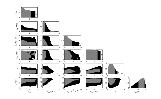
Figure 1: The estimated prior probability density for the entropy-based model parameters. The constraints arise from the underlying assumptions about the cluster physics. The prior ranges encompass typical values of these parameters observed to date. The grey scale represents estimates of the 68 and 95 per cent intervals.

4.2 Mock X-ray surface brightness data

The X-ray surface brightness is calculated from the known electron density and temperature distribution of a simulated cluster by using Equation 19. The resulting surface brightness map is then multiplied by the count rate conversion factor of a typical instrument (the EPIC camera on XMM-Newton), which is assumed to be constant across the 0.5-2 keV energy band. We use a typical neutral hydrogen column density of $10^{20}\,\mathrm{cm}^{-2}$, and an integration time equal to 10 ks. The map is then multiplied by the solid angle per pixel ($\Delta\Omega$) to convert the data to the expected counts per pixel. The number of counts on each pixel is then related to the surface brightness and the pixel solid angle by the following expression

$$N_{\mathrm{cnts}}=\left({S_{\mathrm{X}}\over\mathrm{erg}\,\mathrm{s}^{-1}\,\mathrm{cm}^{-2}\,\mathrm{sr^{-1}}}\right)\left(\Delta\Omega\over\mathrm{sr}\right)5\times 10^{15}\,\mathrm{cnts}.$$ (29)

Noise is introduced into the map by applying the Poisson distribution to each pixel, with the mean equal to the photon count. For the purposes of the mock observation we do not take into account the point spread function, the effect of which is assumed to be insignificant on the cluster scales that are being modelled. We also do not the take into account the residual background X-ray emission which would need to be considered for a real observation.

The X-ray surface brightness profile data are then constructed by binning the photon counts map into 5 arcsec radial bins and converting from counts to physical units. The error in the mean value associated with each bin is just the square root of the bin value divided by the number of pixels that contributed to that radial bin. Hence at moderately large radii the number of pixels contributing to each bin is large and so the statistics can be approximated by a Gaussian distribution.

5 Results

5.1 The Prior

It is important to first understand the intrinsic constraints introduced by the prior before performing a joint fit to the data. The prior includes both the volume of the parameter space being considered and the assumptions upon which the model is based. Figure 1 shows the estimated prior distribution for each of the parameters in the entropy-based model. This plot was constructed by running the analysis pipeline with all of the model constraints in place, but with no SZ or X-ray surface brightness data. The MCMC chains are allowed to search parameter space within the constraints of the model until a large number of samples are generated ($\sim 100,000$) and thus produce a reasonable estimation of the prior distribution.

Constraints on the parameters arise from the assumption that the intra-cluster medium is in hydrostatic equilibrium and that the pressure profile must be physical at all radii. The model also prefers higher central electron temperature values due to the constraint on the pressure. In order for the condition of hydrostatic equilibrium to be satisfied, large mass values can only correlate to relatively high temperatures, and this will provide a constraint on the value of $r_{\mathrm{DM}}$ which is seen in the figure. The nature of interferometric data is such that they are not able to constrain a signal that is non-varying over the angular scales to which the instrument is sensitive. Therefore in the case of low signal-to-noise data it would be possible to obtain solutions within the acceptable prior range of the model, where the temperature increases rapidly at large radii and while the density profile decreases, leading to an SZ signal with a large constant additive component. To avoid this clearly unphysical situation we impose the constraint that the electron temperature must either be constant or decreasing at radii larger than the virial radius. The principal effect of this constraint is to significantly reduce the probability of having an nonphysical high value for the entropy power law parameter $\alpha$ at large radii.

5.2 Self-Consistency

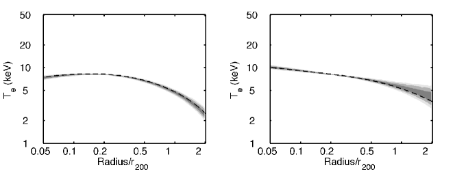
Figure 2: The estimated posterior probability density for the temperature as a function of radius, from joint fitting the entropy-based model to mock high signal-to-noise CBI2 SZ and X-ray surface brightness data, for cool core (left) and non-cool core (right) clusters constructed from the entropy-based model. The grey scale represents the 68, 95 and 99 per cent intervals. The dashed lines represent the true simulation values.

We construct mock CBI2 SZ and X-ray surface brightness data from the entropy-based model in order to test that, given idealised high signal-to-noise, the correct values for cluster properties can be returned from model fitting to the data. Two spherically-symmetric model clusters are constructed for the self-consistency test, one with a cool-core and the other with a non-cool core. For this test the data have high signal-to-noise and the intrinsic CMB features are not included in the SZ signal. The estimated posterior probability density for the temperature profile of each model cluster is shown in Figure 2. The results show that correct unbiased estimates of the cluster properties are reproduced by fitting the entropy-based model to idealised data constructed from the same model.

5.3 Hydrodynamic/N-body Simulations

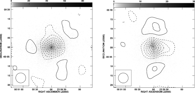
Figure 3: Mock observations of the X-ray surface brightness (grey-scale) and SZ temperature decrement (contours), for the simulated clusters FB1 (left) and FB3 (right) from Kay et al. (2008). The grey-scale is in units of counts per pixel for a generic X-ray observation. The contours represent multiples of the 2 $\sigma$ noise level from a typical 31 GHz observation using the CBI2 array. The full-width half-maximum of the CBI2 synthesised beam is indicated in the bottom left-hand corner of each map.

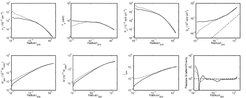
Figure 4: The physical properties of the simulated clusters FB1 (dashed line) and FB3 (solid line) as a function of radius. The dot-dashed line in the frame showing the radial entropy represents the power law predicted by simulations. The dot-dashed line in the frame showing the ratio of the pressure gradient to gravity represents a cluster in hydrostatic equilibrium. FB1 is cool-core relaxed cluster and FB3 is non cool-core.

Cosmological $N$-body/hydrodynamic simulations of two clusters from Kay et al. (2008) are used to test the entropy-based model. The simulations were run the with the Gadget2 code (Springel et al., 2005) that uses the Particle-Mesh and tree algorithms to calculate gravitational forces and Smoothed Particle Hydrodynamics to model the gas. Additionally, the gas was allowed to cool radiatively, leading to a decrease in entropy, and form collisionless stars at low temperature ($T<10^{5}$ K) and high density ($n_{\mathrm{H}}>10^{-3}\mathrm{cm^{-3}}$). Thermal energy was also injected into such regions (feedback) leading to a large increase in the entropy of the local gas. This phenomenological approach to re-heating and galaxy formation in the cluster was found by Kay et al. (2004) to reproduce the observed $L_{\mathrm{X}}-T_{\mathrm{X}}$ relation, and so provides a good test for the entropy-based model. The sub-sample used in this work consists of two clusters with similar total masses ($\sim 10^{15}$ M_⊙) and temperatures ($\sim 5$ keV), but with quite different merger histories. FB1 has a cool core and is in a relaxed state, while FB3 is a non-cool core cluster and recently underwent a strong merger at $z\sim 0.4$. Therefore our model should not only be able to reproduce the global properties of each cluster, but also correctly constrain the different profiles at large radii.

Maps of $\Delta T_{\mathrm{SZ}}$ (at 31 GHz) and $S_{\mathrm{X}}$ (in the 0.5 - 2.0 keV band) were generated for each cluster by calculating the electron density and temperature properties for every hot particle within a cylinder of length 6 $r_{200}$ and projected radius 3 $r_{200}$. Each particle contribution is smoothed and projected along the length of the cylinder onto a 1024 $\times$ 1024 2D pixel array, using the projected version of the GADGET2 SPH kernel. The SZ decrement and X-ray surface brightnesses were calculated using Equations 15 and 19. The CBI2 SZ and X-ray surface brightness maps for each simulated cluster are shown in Figure 3 with realistic noise applied. Note that, for a fair comparison, the same $\Lambda(T_{\mathrm{e}})$ cooling function is used to generate the simulated X-ray surface brightness map that is also used when producing the aforementioned analytical model. The maps are centred about the most gravitationally-bound dark matter particle and thus the most globally symmetric point. For the relaxed cluster FB1, this coincides with the brightest SZ and X-ray surface brightness points. In the case of FB3, this cluster underwent a recent merger event that has produced an asymmetric core region, and therefore the brightest pixels in the maps are offset from the centre. However the symmetry of the global structure of this cluster is centred about the central pixel of the map and not the fine substructure of the brightest peaks. This therefore acts to flatten the central part of the electron density profile, and hence also the X-ray surface brightness.

The profiles for the physical properties of the simulated clusters are shown in Figure 4. Clusters of galaxies typically depart from hydrostatic equilibrium within their core region due to physical processes other than gravitational collapse, such as disturbance from recent merger activity, pre-heating from active galactic nuclei and radiative cooling. Both simulated clusters exhibit this behaviour within a radius of $\la 100\,\mathrm{kpc}$, and their gas properties diverge considerably in this region. We therefore choose to ignore the central cluster core in fitting to the data since the high gas density, and hence X-ray surface brightness, will strongly bias the results.

5.4 Results from simulated data

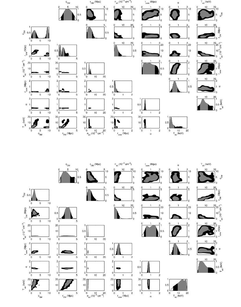
Figure 5: The estimated posterior probability density for the entropy-based model parameters from separately fitting to simulated high signal-to-noise CBI2 SZ data (top triangle) and X-ray surface brightness data (bottom triangle). The top and bottom plots represent fits for cluster FB1 and FB3 respectively. The grey-scale represents the 68 and 95 per cent intervals.

Mock SZ data and X-ray surface brightness data are constructed from the simulated cluster maps using the method described in sections 4.1 and 4.2. We fit the entropy-based model to both high and low signal-to-noise simulated data in order to investigate possible systematics introduced into the derived cluster properties. For the high signal-to-noise case we fit to idealised data with very low experimental error, no calibration errors, and no intrinsic CMB signal in the SZ data. Conversely for low signal-to-noise data we simulate larger experimental error, and introduce calibration error and an intrinsic CMB component in the SZ data. The calibration errors are introduced as nuisance parameters to be marginalised over and are distributed by a Gaussian prior with $\sigma_{\mathrm{cal}}$ given by the quoted error value. A calibration error of 5 per cent is used for the SZ data, typical of the calibration of CBI2 visibility data, and the X-ray surface brightness data typically contain a calibration error of 10 per cent (Andersson & Madejski, 2004).

Figure 5 shows the constraints introduced from separately fitting to high signal-to-noise SZ and X-ray data. The SZ data constrain the integrated line-of-sight pressure and therefore generate an anti-correlation between the central electron density and temperature parameters. In addition the SZ data reduce the likelihood of having large central electron density and temperature values since these would generate large SZ signals that are inconsistent with the data. The X-ray surface brightness data are proportional to the integrated square of the line-of-sight electron density and therefore strongly constrain the central electron density parameter. The X-ray data is of relatively higher resolution than the SZ data and is therefore much more dependent upon the shape of the entropy profile providing strong constraints on $r_{\mathrm{core}}$ and $\alpha$. The high signal-to-noise surface brightness data do not provide a strong constraint on the temperature and mass of the cluster. In the case of FB1 the X-ray surface brightness data appear to generate a series of high likelihood peaks within parameter space. However the data are unable to distinguish between these in the absence of an additional constraint from the SZ data.

Name	Data	$Y_{\mathrm{200}}\,D_{\mathrm{A}}^{2}$	$M_{\mathrm{200}}$	$f_{\mathrm{gas,200}}$
FB1	Simulation	0.931	11.6	0.094
	High S/N	$0.986^{+0.011}_{-0.016}$	$11.4^{+0.2}_{-0.3}$	$0.098^{+0.003}_{-0.002}$
	Low S/N	$1.25^{+0.41}_{-0.133}$	$15.8^{+3.8}_{-5.1}$	$0.064^{+0.016}_{-0.009}$
FB3	Simulation	0.863	10.7	0.096
	High S/N	$0.89^{+0.03}_{-0.02}$	$11.3^{+0.4}_{-0.4}$	$0.091^{+0.002}_{-0.003}$
	Low S/N	$1.05^{+0.40}_{-0.23}$	$15.8^{+5.0}_{-5.4}$	$0.064^{+0.020}_{-0.020}$

Table 1: Results from joint entropy-based model fits to the simulated clusters. Column 1 gives the cluster name; column 2 the data description; column 3 the integrated comptonisation within the virial radius, in units of $10^{-4}\,\mathrm{Mpc}^{2}$; column 4 the total mass within the virial radius, in units of $10^{14}\,M_{\odot}$, column 5 the gas mass fraction within the virial radius. Errors represent the 68 per cent interval.

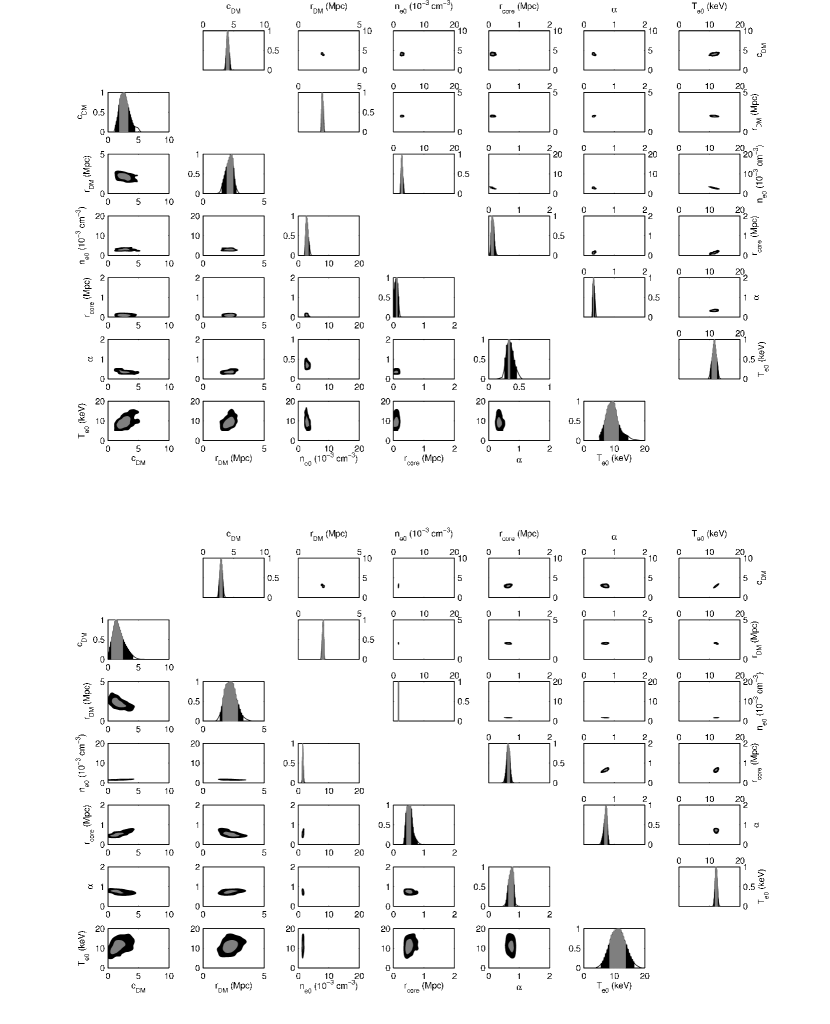
Figure 6: The estimated posterior probability density for the entropy-based model parameters from joint fitting to simulated high signal-to-noise (top triangle) and low signal-to-noise (bottom triangle) CBI2 SZ and X-ray data. The top and bottom plots represent fits for clusters FB1 and FB3 respectively. The grey-scale represents the 68 and 95 per cent intervals.

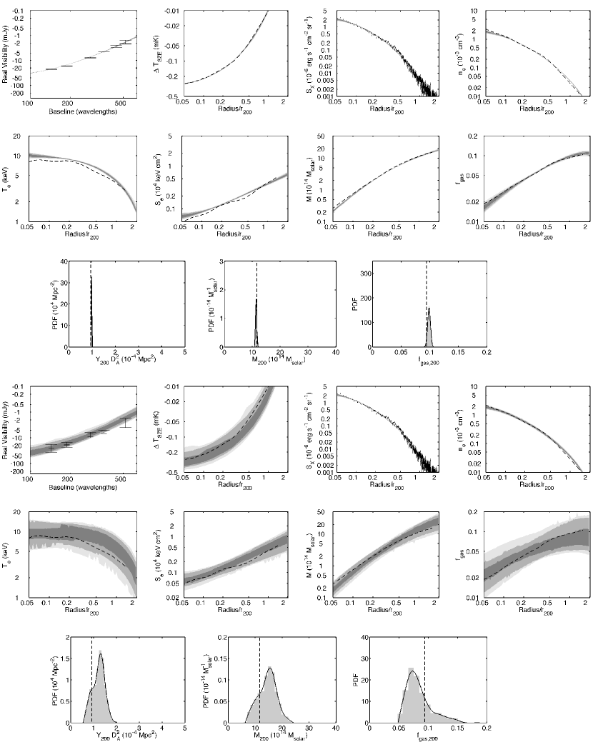
Figure 7: The estimated posterior probability density for properties of Cluster FB1 from joint fitting the entropy-based model to simulated high signal-to-noise (top) and low signal-to-noise (bottom) CBI2 SZ and X-ray data for cluster FB1. The grey scale represents the 68, 95 and 99 per cent intervals. The dashed lines represent the true simulation values and the error-bars the mock data.

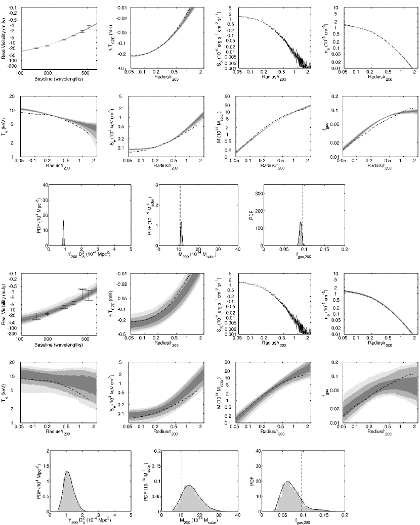
Figure 8: continued

Cluster FB3.

Results from fitting simultaneously to both data sets, for both the high and low signal-to-noise cases, are shown in Table 1 and Figures 6 and 7, where estimates of the posterior distribution for the model parameters, profiles of the cluster properties and selected enclosed quantities are plotted.

The model parameters are constrained by the combination of both data sets. For the purposes of comparison with the known simulated cluster properties the radial profiles are scaled by the known true $r_{200}$ value, and all global quantities are calculated by integrating within this radius. In the high signal-to-noise regime the radial profiles and global parameters of the true physical properties are reproduced well by the parametric fit, with systematic error $<10$ per cent at $r_{200}$. This result is fairly consistent with Kay et al. (2004), who find that the hydrostatic mass estimated from a combination of $\beta$ model fits to the X-ray surface brightness data and spatial temperature information agrees to within $10$ per cent ($r\la r_{500}$) for the simulated clusters which contain feedback. They find that the presence of feedback produces a higher degree of thermalisation than if the cluster were simply described by a non-radiative model and so the estimated mass is close to the true value. In the low signal-to-noise regime the increase in noise leads to much larger widths in the probability distributions of the cluster quantities and, while shifting the peaks of the distributions, are still consistent with the known simulation values within the errors.

Table 2 gives the natural logarithm of the evidence for different models given the data. The evidence values for both low and high signal-to-noise regimes support the inclusion of hyper-parameters. The ratios of best fit values for the SZ and X-ray hyper-parameters in each regime are 15:1 and 3.5:1 (high signal-to-noise), and 2.5:1 and 1.1:1 (low signal-to-noise), for FB1 and FB3 respectively, indicating that the hyper-parameters weight the likelihood in favour of the SZ data. While the CBI2 SZ data are insensitive to variation on scales smaller than 500 kpc, the X-ray data are much more sensitive to variations over this range. The nature of the parametric model is such that it is inherently smooth on these smaller scales; hence clumping of the gas will deviate the model from the X-ray data, while still producing a relatively good fit to the SZ data. Therefore the weights will typically favour the SZ data relative to the X-ray surface brightness. In the case of the FB3 data, the relative weightings are more similar since the X-ray data are a closer match to the model over the considered radius range. A reduction in signal-to-noise leads to a decrease in the ratios of hyper-parameters for each cluster, and so both the SZ and X-ray data sets provide a more consistent match to the model.

5.5 Comparison with the isothermal $\beta$ model

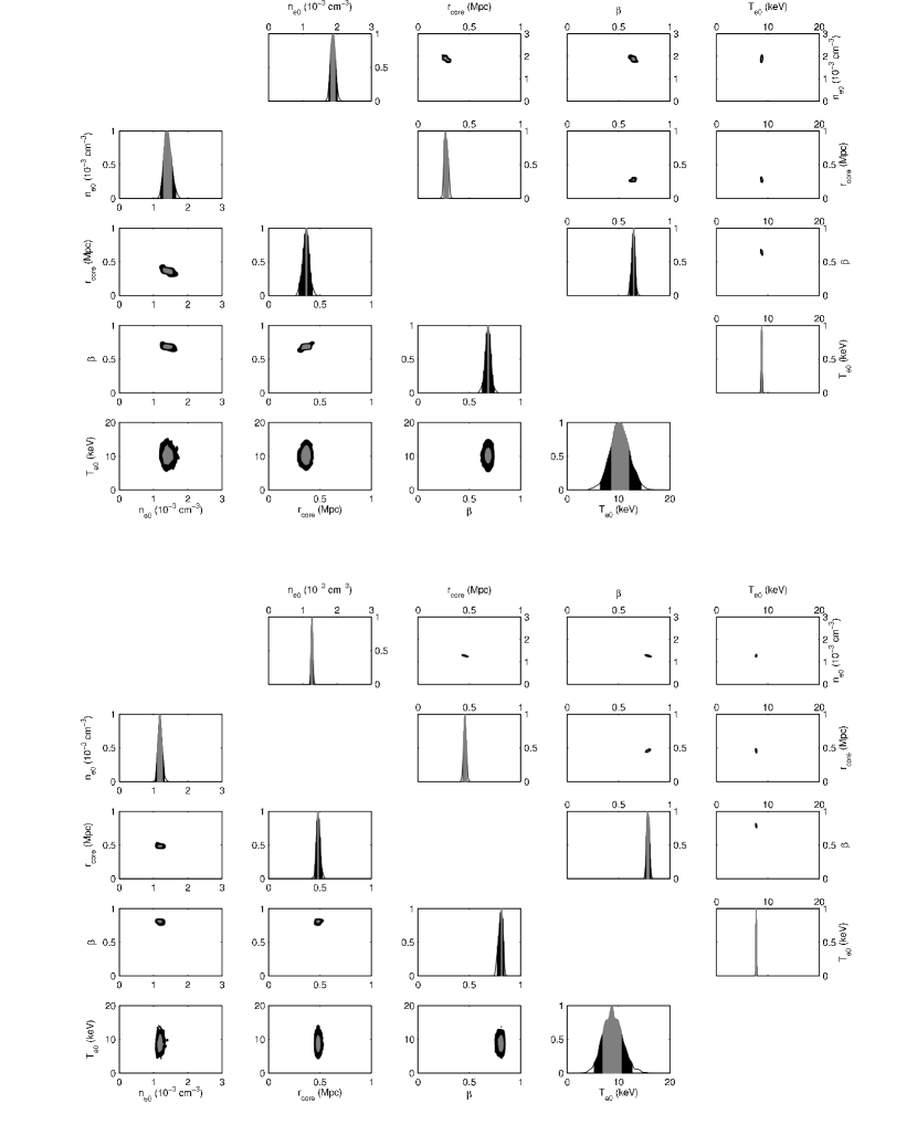
Figure 9: The estimated posterior probability density for the isothermal $\beta$ model parameters from joint fitting to simulated high signal-to-noise (top triangle) and low signal-to-noise (bottom triangle) CBI2 SZ and X-ray data. The top and bottom plots represent fits for clusters FB1 and FB3 respectively. The grey-scale represents the 68 and 95 per cent intervals.

Figure 10: The estimated posterior probability density for properties of Cluster FB1 from joint fitting the isothermal $\beta$ model to simulated high signal-to-noise (top) and low-signal-to-noise (bottom) CBI2 SZ and X-ray data for cluster FB1. The grey scale represents the 68, 95 and 99 per cent intervals. The dashed lines represent the true simulation values and the error-bars the mock data.

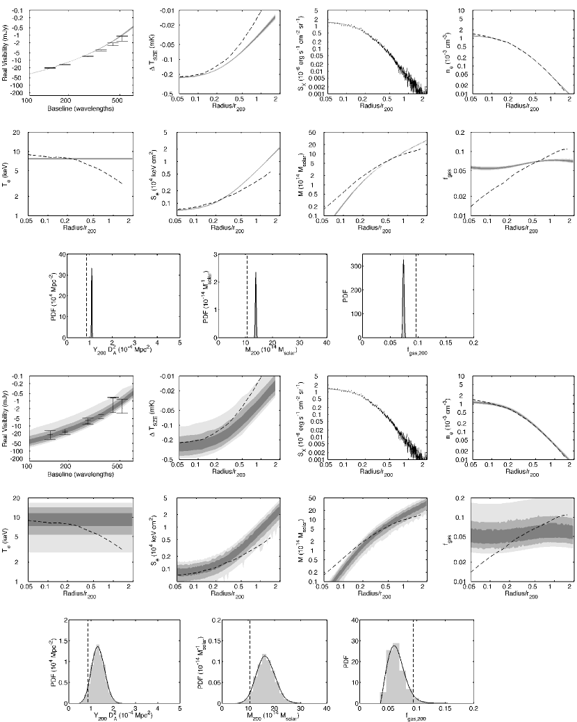
Figure 11: continued

Cluster FB3.

Even though the simulated clusters are clearly not isothermal, for the purposes of comparison to previous work and to demonstrate the systematic differences in derived cluster properties using the two different models, we perform joint fits using the single isothermal $\beta$ model. The electron density and temperature are then given by

$$n_{\mathrm{e}} = n_{\mathrm{e0}}\left(1+\left({r\over r_{\mathrm{core}}}\right)^{2}\right)^{-3\beta/2}$$ (30)

$$T_{\mathrm{e}} = T_{\mathrm{e0}},$$ (31)

where $n_{\mathrm{e0}}$ and $T_{\mathrm{e0}}$ are the central electron density and temperature respectively, $r_{\mathrm{core}}$ is the core radius, and $\beta$ is a parameter that determines the large scale behaviour of the electron density.

Figures 9 and 10 show the resulting posterior distributions for the model parameters, the profiles, and global values within $r_{200}$. There is a strong systematic difference between the estimated and true simulation values when using this model, resulting from over-estimates of the electron temperature and SZ decrement. The result is a systematic over-estimate of the total mass of $\sim$ 20 per cent at $r_{200}$ and an under-estimate of the total mass at $r<r_{500}$. These results are consistent with the findings by Kay et al. (2004) who measure similar errors in estimating the total mass based upon the isothermal model. The systematic error in derived cluster properties is seen in both the high and low signal-to-noise scenarios, and therefore the introduction of both thermal noise and intrinsic CMB anisotropy is not enough to dominate over the effects of the intrinsic isothermal $\beta$ model discrepancy with the simulations.

It is informative to compare the relative quality of the fit that the entropy-based and single isothermal $\beta$ models give, based upon their respective logarithmic evidence values. In almost all the cases the evidence for the isothermal $\beta$ model is significantly lower than that of the entropy-based model, with the exception of the low signal-to-noise scenario for the FB3 simulated cluster. This is due to the flat core nature of the X-ray surface brightness profile for this cluster, as a result of the displacement of the gas peak in the central region. As such when significantly lower signal-to-noise data is used the isothermal $\beta$ model, with its flat core behaviour at small radii, provides an equally good fit (if not slightly better) than the entropy-based model. However in the case of the FB1 simulated cluster, the X-ray profile is strongly peaked in the central region and therefore the isothermal $\beta$ model provides a significantly poorer fit to both high and low signal-to-noise data. This can be seen upon visual inspection of the electron density profiles for FB1 in Figure 10, where the isothermal $\beta$ model fails to provide a suitable fit at both small and large radii.

The evidence values in Table 2 support the inclusion of hyper-parameters in both the high and low signal-to-noise scenarios for the isothermal $\beta$ model. The relative weightings of each the SZ and X-ray data sets are to 30:1 (FB1) and 3:1 (FB3) for the high signal-to-noise data, and 4:1 and 1.1:1 for the corresponding low signal-to-noise data. The likelihood calculation is therefore weighted in favour of the SZ data, except in the case of the low signal-to-noise FB3 data where both are almost equally favoured.

		High SNR		Low SNR
Name	Model	$\mathcal{M}_{0}$	$\mathcal{M}_{1}$	$\mathcal{M}_{0}$	$\mathcal{M}_{1}$
FB1	Entropy	6113	6476	4757	4764
	Isothermal $\beta$	5946	6405	4559	4724
FB3	Entropy	6147	6273	4807	4816
	Isothermal $\beta$	6131	6231	4810	4817

Table 2: The natural logarithm of the evidence (the probability of the data given a particular parametric model, see Equation 23) for high and low signal-to-noise CBI2 SZ and X-ray surface brightness data. Note that the absolute value of the evidence is dependent upon the data, and so the quantity of interest is the difference between these values. Models that include SZ and X-ray hyper-parameters are represented by $\mathcal{M}_{1}$ and those that do not are represented by $\mathcal{M}_{0}$.

6 Discussion and Conclusions

We have developed a parametric model for the gas in galaxy clusters, based on three physical assumptions: the dark matter follows an NFW profile, the gas entropy can be described by a power law with a flattened core, and the gas is in hydrostatic equilibrium. Using entropy rather than, for example, the gas density as the basic parametrization is motivated by the theoretical and observed self-similarity of entropy profiles in cluster samples. This model can be constrained by SZ and X-ray data to give fitted gas and total matter properties of the cluster. The model has sensible convergence properties and can be used out to the virial radius of the cluster. By construction, the model does not allow unphysical or inconsistent properties of the cluster gas as can happen if, for example, a parametric fit to the gas density is combined with an unrelated parametric fit to the temperature.

We have tested the model using two detailed N-body plus hydrodynamical simulations of massive clusters with contrasting merger histories. In both cases, using realistic mock data from presently available X-ray and SZ telescopes, the model is able to accurately fit both the integrated cluster parameters and their radial profiles. If high-quality data with very low noise are simulated, the cluster parameters are returned with essentially no bias. Our fitting code includes both random noise and systematic calibration errors in the data and fully includes the effect of contamination from primordial CMB fluctuations and radio sources in the SZ data. We also use a hyper-parameter approach to scale the relative constraints from the two data sets. Comparison with the widely-used isothermal $\beta$ model confirms previous results that this model can result in significant biases in fitted cluster parameters (e.g. Kay et al., 2004; Hallman et al., 2007). The quality of the available SZ data is now high enough to require a more sophisticated modelling approach, especially with data that are sensitive to the outskirts of cluster.

This model however remains simplistic in several potentially important ways. The assumption of hydrostatic equilibrium is clearly broken badly in the central cores of clusters, and we are forced to ignore the data in this region. Hydrostatic equilibrium will also be broken in the main body of the cluster due to bulk motions and other non-thermal support, although in our simulations this does not seem to be a significant impediment to measuring accurate cluster profiles. We do not currently treat the boundary of the cluster in a fully consistent way – at some radius the virialised gas must meet a boundary shock of in-falling material and we do not model the corresponding step in pressure. We also do not yet consider additional observation constraints such as X-ray spectral and optical weak lensing measurements, although these are in principle straightforward to incorporate in to our analysis framework.

In subsequent papers we will use this model to analyse SZ data from the CBI2 experiment jointly with relevant X-ray imaging data.

References

- Allen et al. (2001) Allen S. W., Schmidt R. W., Fabian A. C., 2001, MNRAS, 328, L37
- Ameglio et al. (2007) Ameglio S., Borgani S., Pierpaoli E., Dolag K., 2007, MNRAS, 382, 397
- Ameglio et al. (2009) Ameglio S., Borgani S., Pierpaoli E., Dolag K., Ettori S., Morandi A., 2009, MNRAS, 394, 479
- Andersson & Madejski (2004) Andersson K. E., Madejski G. M., 2004, ApJ, 607, 190
- Arnaud et al. (2010) Arnaud M., Pratt G. W., Piffaretti R., Böhringer H., x Croston J. H., Pointecouteau E., 2010, AAP, 517, A92+
- Atrio-Barandela et al. (2008) Atrio-Barandela F., Kashlinsky A., Kocevski D., Ebeling H., 2008, ApJ, 675, L57
- Bautz et al. (2009) Bautz M. W., Miller E. D., Sanders J. S., Arnaud K. A., Mushotzky R. F., Porter F. S., Hayashida K., Henry J. P., Hughes J. P., Kawaharada M., Makashima K., Sato M., Tamura T., 2009, PASJ, 61, 1117
- Birkinshaw (1999) Birkinshaw M., 1999, PhysRep, 310, 97
- Bond et al. (2000) Bond J. R., Jaffe A. H., Knox L., 2000, ApJ, 533, 19
- Bulbul et al. (2010) Bulbul G. E., Hasler N., Bonamente M., Joy M., 2010, ApJ, 720, 1038
- Cavagnolo et al. (2009) Cavagnolo K. W., Donahue M., Voit G. M., Sun M., 2009, ApJS, 182, 12
- Cavaliere & Fusco-Femiano (1976) Cavaliere A., Fusco-Femiano R., 1976, AAP, 49, 137
- Cavaliere & Fusco-Femiano (1978) —, 1978, AAP, 70, 677
- Challinor & Lasenby (1998) Challinor A., Lasenby A., 1998, ApJ, 499, 1
- Donahue et al. (2006) Donahue M., Horner D. J., Cavagnolo K. W., Voit G. M., 2006, ApJ, 643, 730
- George et al. (2009) George M. R., Fabian A. C., Sanders J. S., Young A. J., Russell H. R., 2009, MNRAS, 395, 657
- Grego et al. (2000) Grego L., Carlstrom J. E., Joy M. K., Reese E. D., Holder G. P., Patel S., Cooray A. R., Holzapfel W. L., 2000, ApJ, 539, 39
- Grego et al. (2001) Grego L., Carlstrom J. E., Reese E. D., Holder G. P., Holzapfel W. L., Joy M. K., Mohr J. J., Patel S., 2001, ApJ, 552, 2
- Hallman et al. (2007) Hallman E. J., Burns J. O., Motl P. M., Norman M. L., 2007, ApJ, 665, 911
- Hobson et al. (2002) Hobson M. P., Bridle S. L., Lahav O., 2002, MNRAS, 335, 377
- Hoshino et al. (2010) Hoshino A., Patrick Henry J., Sato K., Akamatsu H., Yokota W., Sasaki S., Ishisaki Y., Ohashi T., Bautz M., Fukazawa Y., Kawano N., Furuzawa A., Hayashida K., Tawa N., Hughes J. P., Kokubun M., Tamura T., 2010, PASJ, 62, 371
- Itoh et al. (1998) Itoh N., Kohyama Y., Nozawa S., 1998, ApJ, 502, 7
- Kawaharada et al. (2010) Kawaharada M., Okabe N., Umetsu K., Takizawa M., Matsushita K., Fukazawa Y., Hamana T., Miyazaki S., Nakazawa K., Ohashi T., 2010, ApJ, 714, 423
- Kay (2004) Kay S. T., 2004, MNRAS, 347, L13
- Kay et al. (2008) Kay S. T., Powell L. C., Liddle A. R., Thomas P. A., 2008, MNRAS, 386, 2110
- Kay et al. (2004) Kay S. T., Thomas P. A., Jenkins A., Pearce F. R., 2004, MNRAS, 355, 1091
- Komatsu & Seljak (2001) Komatsu E., Seljak U., 2001, MNRAS, 327, 1353
- Kosowsky (2003) Kosowsky A., 2003, New Astronomy Review, 47, 939
- LaRoque et al. (2006) LaRoque S. J., Bonamente M., Carlstrom J. E., Joy M. K., Nagai D., Reese E. D., Dawson K. S., 2006, ApJ, 652, 917
- Lloyd-Davies et al. (2000) Lloyd-Davies E. J., Ponman T. J., Cannon D. B., 2000, MNRAS, 315, 689
- Mahdavi et al. (2007) Mahdavi A., Hoekstra H., Babul A., Sievers J., Myers S. T., Henry J. P., 2007, ApJ, 664, 162
- Mason et al. (2003) Mason B. S., Pearson T. J., Readhead A. C. S., Shepherd M. C., Sievers J., Udomprasert P. S., Cartwright J. K., Farmer A. J., Padin S., Myers S. T., Bond J. R., Contaldi C. R., Pen U., Prunet S., Pogosyan D., Carlstrom J. E., Kovac J., Leitch E. M., et. al., 2003, ApJ, 591, 540
- Mitchell et al. (2009) Mitchell N. L., McCarthy I. G., Bower R. G., Theuns T., Crain R. A., 2009, MNRAS, 395, 180
- Morandi & Ettori (2007) Morandi A., Ettori S., 2007, MNRAS, 380, 1521
- Mroczkowski et al. (2009) Mroczkowski T., Bonamente M., Carlstrom J. E., Culverhouse T. L., Greer C., Hawkins D., Hennessy R., Joy M., Lamb J. W., Leitch E. M., Loh M., Maughan B., Marrone D. P., Miller A., Muchovej S., Nagai D., et. al., 2009, ApJ, 694, 1034
- Muchovej et al. (2007) Muchovej S., Mroczkowski T., Carlstrom J. E., Cartwright J., Greer C., Hennessy R., Loh M., Pryke C., Reddall B., Runyan M., Sharp M., Hawkins D., Lamb J. W., Woody D., Joy M., Leitch E. M., Miller A. D., 2007, ApJ, 663, 708
- Nagai et al. (2007) Nagai D., Kravtsov A. V., Vikhlinin A., 2007, ApJ, 668, 1
- Navarro et al. (1995) Navarro J. F., Frenk C. S., White S. D. M., 1995, MNRAS, 275, 720
- Navarro et al. (1996) —, 1996, ApJ, 462, 563
- Navarro et al. (1997) —, 1997, ApJ, 490, 493
- Nord et al. (2009) Nord M., Basu K., Pacaud F., Ade P. A. R., Bender A. N., Benson B. A., Bertoldi F., Cho H., Chon G., Clarke J., Dobbs M., Ferrusca D., Halverson N. W., Holzapfel W. L., Horellou C., Johansson D., Kennedy J., Kermish Z., et. al., 2009, AAP, 506, 623
- Ostriker et al. (2005) Ostriker J. P., Bode P., Babul A., 2005, ApJ, 634, 964
- Padin et al. (2002) Padin S., Shepherd M. C., Cartwright J. K., Keeney R. G., Mason B. S., Pearson T. J., Readhead A. C. S., Schaal W. A., Sievers J., Udomprasert P. S., Yamasaki J. K., Holzapfel W. L., Carlstrom J. E., Joy M., Myers S. T., Otarola A., 2002, PASP, 114, 83
- Piffaretti et al. (2005) Piffaretti R., Jetzer P., Kaastra J. S., Tamura T., 2005, AAP, 433, 101
- Pointecouteau et al. (2004) Pointecouteau E., Arnaud M., Kaastra J., de Plaa J., 2004, AAP, 423, 33
- Ponman et al. (1999) Ponman T. J., Cannon D. B., Navarro J. F., 1999, Nature, 397, 135
- Ponman et al. (2003) Ponman T. J., Sanderson A. J. R., Finoguenov A., 2003, MNRAS, 343, 331
- Pratt et al. (2010) Pratt G. W., Arnaud M., Piffaretti R., Böhringer H., Ponman T. J., Croston J. H., Voit G. M., Borgani S., Bower R. G., 2010, AAP, 511, A85+
- Pratt et al. (2006) Pratt G. W., Arnaud M., Pointecouteau E., 2006, AAP, 446, 429
- Pratt et al. (2007) Pratt G. W., Böhringer H., Croston J. H., Arnaud M., Borgani S., Finoguenov A., Temple R. F., 2007, AAP, 461, 71
- Raymond & Smith (1977) Raymond J. C., Smith B. W., 1977, ApJS, 35, 419
- Reese et al. (2002) Reese E. D., Carlstrom J. E., Joy M., Mohr J. J., Grego L., Holzapfel W. L., 2002, ApJ, 581, 53
- Ruhl et al. (2004) Ruhl J., Ade P. A. R., Carlstrom J. E., Cho H.-M., Crawford T., Dobbs M., Greer C. H., Halverson N. w., Holzapfel W. L., Lanting T. M., Lee A. T., Leitch E. M., Leong J., Lu W., Lueker M., Mehl J., Meyer S. S., Mohr J. J., et al., 2004, in Society of Photo-Optical Instrumentation Engineers (SPIE) Conference Series, Vol. 5498, Society of Photo-Optical Instrumentation Engineers (SPIE) Conference Series, C. M. Bradford, P. A. R. Ade, J. E. Aguirre, J. J. Bock, M. Dragovan, L. Duband, L. Earle, J. Glenn, H. Matsuhara, B. J. Naylor, H. T. Nguyen, M. Yun, & J. Zmuidzinas, ed., pp. 11–29
- Seljak & Zaldarriaga (1996) Seljak U., Zaldarriaga M., 1996, ApJ, 469, 437
- Sievers et al. (2009) Sievers J. L., Mason B. S., Weintraub L., Achermann C., Altamirano P., Bond J. R., Bronfman L., Bustos R., Contaldi C., Dickinson C., Jones M. E., May J., Myers S. T., Oyarce N., Padin S., Pearson T. J., Pospieszalski M., et. al., 2009, ArXiv e-prints
- Sivia (2006) Sivia D. S., 2006, Data Analysis: A Bayesian Tutorial., 2nd edn. Oxford University Press, New York
- Skilling (2004) Skilling J., 2004, http://www.inference.phy.cam.ac.uk/bayesys/
- Springel et al. (2005) Springel V., White S. D. M., Jenkins A., Frenk C. S., Yoshida N., Gao L., Navarro J., Thacker R., Croton D., Helly J., Peacock J. A., Cole S., Thomas P., Couchman H., Evrard A., Colberg J., Pearce F., 2005, Nature, 435, 629
- Sunyaev & Zel’dovich (1970) Sunyaev R. A., Zel’dovich Y. B., 1970, Ap&SS, 7, 3
- Tozzi & Norman (2001) Tozzi P., Norman C., 2001, ApJ, 546, 63
- Udomprasert et al. (2004) Udomprasert P. S., Mason B. S., Readhead A. C. S., Pearson T. J., 2004, ApJ, 615, 63
- Vikhlinin et al. (2006) Vikhlinin A., Kravtsov A., Forman W., Jones C., Markevitch M., Murray S. S., Van Speybroeck L., 2006, ApJ, 640, 691
- Voit et al. (2005) Voit G. M., Kay S. T., Bryan G. L., 2005, MNRAS, 364, 909
- Zhang et al. (2008) Zhang Y.-Y., Finoguenov A., Böhringer H., Kneib J.-P., Smith G. P., Kneissl R., Okabe N., Dahle H., 2008, AAP, 482, 451
- Zwart et al. (2008) Zwart J. T. L., Barker R. W., Biddulph P., Bly D., Boysen R. C., Brown A. R., Clementson C., Crofts M., Culverhouse T. L., Czeres J., Dace R. J., Davies M. L., D’Alessandro R., Doherty P., Duggan K., et. al., 2008, MNRAS, 391, 1545