Percolation in living neural networks

Abstract

We study living neural networks by measuring the neurons’ response to a global electrical stimulation. Neural connectivity is lowered by reducing the synaptic strength, chemically blocking neurotransmitter receptors. We use a graph–theoretic approach to show that the connectivity undergoes a percolation transition. This occurs as the giant component disintegrates, characterized by a power law with critical exponent $\beta\simeq 0.65$. $\beta$ is independent of the balance between excitatory and inhibitory neurons and indicates that the degree distribution is gaussian rather than scale free.

Representing complex structures as connected graphs yields a simplification that retains much of their functionality. It is therefore natural that network connectivity emerges as the fundamental feature determining statistical properties, including the existence of power laws, clustering coefficients and the small world phenomenon Barabasi-2002 . While experimental access to man–made networks such as the WWW or e–mail is feasible EckmannMoses-2002 , biological ones such as the genetic networks must be painstakingly revealed node by node HybridProtein-2005 . The connectivity in living neural networks is even more difficult to uncover White-1986 , since connections are hard to identify Markram-2003 ; Chan-2004 and typically differ from brain to brain and from culture to culture Marom-2002 ; Jimbo-1999 . Unraveling the neural wiring diagram even in small cultures, with $\sim 10^{5}$ neurons and $\sim 10^{7}$ connections, is presently not feasible, although some progress has been attained in the study of the link between neural connectivity and information coding Chan-2004 ; Segev-2004 ; Ofer-2006 .

Neural cultures derived from rat hippocampus develop into networks that display bursts of activity, governed by the presence of both excitatory and inhibitory neurons Maeda-1995 ; Marom-2002 . In this Letter we present a novel experimental approach to quantify statistical properties of such networks, and study them in terms of percolation on random graphs Stauffer ; Newman-2001 . We control the connectivity of the entire network, gradually reducing the synaptic strength by means of chemical application. The initially connected network progressively breaks down into smaller clusters until a fully disconnected network is reached. The weakening of the network is quantified and the distribution of sizes of connected components determined by analyzing the neurons’ response to stimulations applied simultaneously to the entire network. Viewed inversely, as the network’s connectivity increases, a percolation transition occurs at a critical synaptic strength with the emergence of a giant component, which increases as a power law with an exponent $\beta\simeq 0.65$.

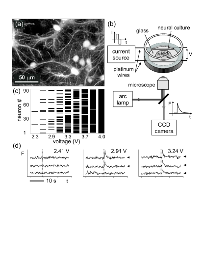
Figure 1: (a) Fluorescence image of a small region of the neural culture. Bright spots are cell bodies. Neural connections, mostly dendrites, are visible. (b) Sketch of the experimental setup. (c) Activity plot of the neural response. Black lines indicate those neurons that respond to the excitation. (d) $F(t)$ signal for 3 neurons at increasing voltages. Vertical lines show the excitation time, and arrows the responding neurons.

Experimental setup and procedure.– Experiments were performed on primary cultures of rat hippocampal neurons, plated on glass coverslips following the procedure described by Papa et al. Papa-1995 (Fig. 1(a)). The cultures were used 14–20 days after plating. The neural network includes $N\simeq 2.5\times 10^{5}$ neurons. The neural culture is placed in a chamber that contains two parallel platinum wires fixed at the bottom and separated by $15$ mm (Fig. 1(b)). The neurons are electrically stimulated by applying a $20$ msec bipolar pulse through the wires. The current is controlled and gradually increased between subsequent pulses, while the corresponding voltage drop $V$ is measured with an oscilloscope. The chamber is mounted on a Zeiss inverted microscope with a $10$X objective, and neuronal activity is monitored using the fluorescent calcium indicator Fluo-4. Images were captured with a cooled charge–coupled device (CCD) camera at a rate of $5$ frames/sec, and processed to record the fluorescence intensity $F$ of a sample of the culture including $n\simeq 400$ individual neurons as a function of time (Fig. 1(d)). The images and the fluorescent signal are further analyzed to reject glia cells Supplementary . Neural spiking activity is detected as a sharp increase of the fluorescence intensity Supplementary .

The connectivity of the network was gradually weakened by adding increasing amounts of CNQX (6-cyano-7-nitroquinoxaline-2,3-dione), the antagonist of the AMPA (alpha-amino-3-hydroxy-5-methyl-4-isoxazolepropionic acid) type receptors in the glutamate synapses of excitatory neurons. NMDA (N-methyl-D-aspartate) receptors were completely blocked with $20$ $\mu$M of the corresponding antagonist APV (2-amino-5-phosphonovalerate), enabling the study of network breakdown due solely to CNQX. To study the role of inhibition, we performed experiments with inhibitory neurons either active or blocked with $40$ $\mu$M of the GABA (Gamma-aminobutyric acid) receptor antagonist bicuculine. From here on, we label the network containing both excitatory and inhibitory neurons by $G_{EI}$, and the network with excitatory neurons only by $G_{E}$.

The response of the network for a given CNQX concentration was measured as the fraction of neurons $\Phi$ that fired in response to the electric stimulation at voltage $V$ (Fig. 1(c)). Response curves $\Phi(V)$ were obtained by increasing the stimulation voltage from $2$ to $6$ V in steps of $0.1-0.5$ V. Between 6 and 10 response curves were measured per experiment, each at a different CNQX concentration. Measurements were completed within 4 h, at the end of which the culture was washed of CNQX to verify that the initial network connectivity was recovered.

Model.– To elucidate the relation between the topology of the living neural network and the observed neural response, we consider a simplified model of the network in terms of bond–percolation on a graph. The neural network is represented by the directed graph $G$. Our main simplifying assumption is the following:  A neuron has a probability $f=f(V)$ to fire as a direct response to the externally applied electrical stimulus, and it always fires if any one of its input neurons fire. This ignores the fact that more than one input is needed to excite a neuron, and that connections are gradually weakened rather than abruptly removed. The model also ignores the presence of feedback loops and recurrent activity in the neural culture. However, we verified with numerical simulations that relaxing these assumptions does not affect the validity of the model Supplementary .

Evidently, the firing probability $\Phi(f)$ increases with the connectivity of $G$, because any neuron along a directed path of inputs may fire and excite all the neurons downstream. All the upstream neurons that can thus excite a certain neuron define its input–cluster or excitation–basin. It is therefore convenient to express the firing probability as the sum over the probabilities $p_{s}$ of a neuron to have an input cluster of size $s-1$,

$$\Phi(f) = f+(1-f)P\left(\text{any input neuron fires}\right)$$ (1)

$$= f+(1-f)\sum_{s=1}^{\infty}p_{s}\left(1-\left(1-f\right)^{s-1}\right)$$

$$= 1-\sum_{s=1}^{\infty}p_{s}\left(1-f\right)^{s},$$

where we used the probability conservation $\sum\nolimits_{s}p_{s}=1$. It is readily seen that $\Phi(f)$ increases monotonically with $f$ and ranges between $\Phi(0)=0$ and $\Phi(1)=1$. The deviation of $\Phi(f)$ from linearity manifests the connectivity of the network (for disconnected neurons $\Phi(f)=f$). Eq. (1) indicates that the observed firing probability $\Phi(f)$ is actually one minus the generating function $H(x)$ (or the $z$–transform) of the cluster–size probability $p_{s}$ Shante-1971 , $H(x)=\sum_{s=1}^{\infty}p_{s}x^{s}=1-\Phi(f)$, where $x=1-f$. One can extract from $H(x)$ the input–cluster size probabilities $p_{s}$, formally by the inverse $z$–transform, or more practically, in the experiment, by fitting $H(x)$ to a polynomial in $x$.

Once a giant component emerges the observed firing pattern is significantly altered. In an infinite network, the giant component always fires no matter what the firing probability $f$ is. This is because even a very small $f$ suffices to excite one of the infinitely many neurons that belong to the giant component. We account for this effect by splitting the neuron population into a fraction $g$ that belongs to the giant component and always fires and the remaining fraction $1-g$ that belongs to finite clusters:

$$\Phi(f) = g+(1-g)\left[f+(1-f)P\left(\text{any inp. neur. fires}\right)\right]$$ (2)

$$= 1-(1-g)\sum_{s=1}^{\infty}p_{s}\left(1-f\right)^{s}.$$

As expected, at the limit of almost no self–excitation $f\rightarrow 0$ only the giant component fires, $\Phi(0)=g$, and $\Phi(f)$ monotonically increases to $\Phi(1)=1$. With a giant component present the relation between $H(x)$ and the firing probability changes, obtaining

$$H(x)=\sum_{s=1}^{\infty}p_{s}x^{s}=1-\Phi(f).$$ (3)

In reality, the giant component is not infinite and it is measured from a sample which has $n$ neurons. Therefore, it fires only after a non–zero, though small, firing probability $f_{T}$ is exceeded. To estimate this finite size threshold we note that when we measure a giant component of size $gn$, then the firing probability is

$$\Phi(f)\simeq g\left(1-\left(1-f\right)^{ng}\right)\simeq g\left(1-e^{-fgn}\right).$$ (4)

This probability becomes significant at the threshold

$$f_{T}\simeq(gn)^{-1}.$$ (5)

Measured network response.– An example of the response curves $\Phi(V)$ for a $G_{EI}$ network with $n=450$ neurons measured at $6$ different concentrations of CNQX is shown in Fig. 2. At one extreme, with [CNQX] $=0$ the network is fully connected, and a few neurons with low firing threshold suffice to activate the entire culture. This leads to a very sharp response curve that approaches a step function, where all neurons form a single cluster that comprises the entire network. At the other extreme, with high concentrations of CNQX ($\simeq$ 10 $\mu$M) the network is completely disconnected, the response curve rises moderately, and is given by the individual neurons’ response. $\Phi(V)$ for individual neurons (denoted as $\Phi_{\infty}(V)$) is well described by an error function $\Phi(V)=0.5+0.5\;\mathrm{erf}\left(\frac{V-V_{0}}{\sqrt{2}\,\sigma_{0}}\right)$. This indicates that the firing threshold of a neuron in the network follows a gaussian distribution with mean $V_{0}$ and width $2\sigma_{0}$.

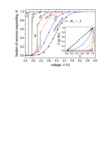
Figure 2: Response curves $\Phi(V)$ for 6 concentrations of CNQX and $n=450$ neurons. The grey bars show the size of the giant component. Lines are a guide to the eye except for $1$ $\mu$M and $10$ $\mu$M that are fits to error functions, with $V_{0}=3.96$ V and $\sigma_{0}=0.46$ V for $10$ $\mu$M. Inset: Corresponding $H(x)$ functions. The bar shows the size of the giant component for $300$ nM.

Intermediate CNQX concentrations induce partial blocking of the synapses. As the network breaks up neurons receive on average fewer inputs and a stronger excitation has to be applied to light up the entire network. The response curves are gradually shifted to higher voltages as [CNQX] increases. Initially, some neurons break off into separated clusters, while a giant cluster still contains most of the remaining neurons. The response curves are then characterized by a big jump that corresponds to the biggest cluster (giant component), and two tails that correspond to smaller clusters of neurons with low or high firing threshold (Fig. 2). Error functions describe these tails well. Beyond these concentrations ([CNQX] $\gtrsim 500$ nM for $G_{EI}$ networks) a giant component cannot be identified and the whole response curve is then also well described by an error function.

Giant component.– The biggest cluster in the network characterizes the giant component, $g$. Experimentally, it is measured as the biggest fraction of neurons that fire together in response to the electric excitation. For each response curve, $g$ is measured as the biggest jump $\Delta\Phi$, as shown by the grey bars in Fig. 2. The size of the giant component is considered to be zero when a characteristic jump cannot be identified, or when the jump is comparable to the noise of the measurement, which is typically about 4% of the number of neurons measured.

We studied the size of the giant component in a range of CNQX concentrations spanning almost three orders of magnitude from $0$ nM to $10$ $\mu$M in logarithmic scale. We define the control parameter $c=1/(1+[\mathrm{CNQX}]/K_{d})$ as a measure of the synaptic strength, where the dissociation constant $K_{d}=300$ nM is the concentration of CNQX at which $50$% of the receptors are blocked Honore-1988 . The parameter $c$ characterizes the connectivity probability between two neurons, and takes values between $0$ (full blocking, independent neurons) and $1$ (full connectivity). Conceptually, it quantifies the number of receptor molecules that are not bound by the antagonist CNQX and therefore are free to activate the synapse.

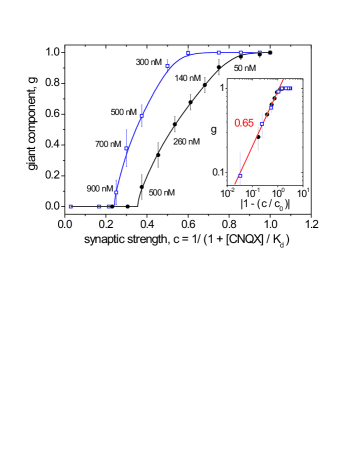
Figure 3: Size of the giant component as a function of the synaptic strength $c$, averaged over $18$ $G_{EI}$ networks ($\bullet$), and $6$ $G_{E}$ networks ($\square$). Lines are a guide to the eye. Some CNQX concentrations are indicated for clarity. Inset: Log–log plot of the power law fits $g\sim|1-c/c_{o}|^{\beta}$. The slope $0.65$ corresponds to the average value of $\beta$ for the two networks.

Fig. 3 shows the breakdown of the network for both $G_{EI}$ and $G_{E}$ networks. The giant component for $G_{EI}$ networks breaks down at much lower CNQX concentrations compared with $G_{E}$ networks, and one can think of the effect of inhibition on the network as effectively reducing the number of inputs that a neuron receives on average. For $G_{EI}$ networks, the giant component vanishes at [CNQX] $\simeq 600$ nM, while for $G_{E}$ networks the critical concentration is around $1000$ nM.

The behavior of the giant component indicates that the neural network undergoes a percolation transition, from a set of small, disconnected clusters of neurons to a giant cluster that contains most of the neurons. At the vicinity of the emergence of the giant component, the percolation transition is described by the power law $g\sim|1-c/c_{o}|^{\beta}$. Power law fits for $G_{EI}$ and $G_{E}$ networks give the same $\beta$ within the experimental error (inset of Fig. 3), with $c_{o}=0.36\pm 0.02$, $\beta=0.66\pm 0.05$ for $G_{EI}$ , and $c_{o}=0.24\pm 0.02$, $\beta=0.63\pm 0.05$ for $G_{E}$ .

Cluster distribution analysis.– The construction of the experimental function $H(x)$ defined in Eq. (3) allows the fit of a polynomial $\sum\nolimits_{s}p_{s}x^{s}$ to determine the size distribution $p_{s}(s)$ for clusters that do not belong to the giant component. Since $f\equiv\Phi_{\infty}(V)$ is the response curve for individual neurons (Fig. 2) and $x=1-f$, the function $H(x)$ for each response curve is obtained by plotting $1-\Phi(V)$ as a function of $1-\Phi_{\infty}(V)$. For curves with a giant component present, its contribution is eliminated and the resulting curve normalized by the factor $1-g$.

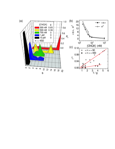
Figure 4: (a) Cluster size distribution $p_{s}(s)$ for the experiment shown in Fig. 2. (b) Average cluster size, $\langle s\rangle$, and variance of the cluster size distribution, $\sigma^{2}=\langle s^{2}\rangle-\langle s\rangle^{2}$, as a function of the concentration of CNQX, averaged over $15$ $G_{EI}$ networks. (c) Giant component firing threshold $f_{T}$ as a function of $1/g$ for two groups of experiments with $90$ ($\square$) and $400$ ($\blacksquare$) neurons measured, and for CNQX concentrations between $0$ and $500$ nM. Lines are least square fits.

The inset of Fig. 2 shows $H(x)$ for the response curves shown in the same figure. The corresponding $p_{s}(s)$ distributions, shown in Fig. 4(a), are obtained from polynomial fits up to order $20$ Supplementary . Since the cluster analysis is sensitive to experimental resolution, it is limited to $g\lesssim 0.8$, which corresponds to [CNQX] $\gtrsim 200$ nM for $G_{EI}$ networks. Experimental resolution also limits the observation of very small clusters for [CNQX] $\lesssim 500$ nM, since they are associated with values of $\Phi(V)$ close to 1 Supplementary . Hence, the cluster size distribution of Fig. 4(a) shows the correct behavior, but not the precise details. Overall, as shown in Fig. 4(b), the clusters start out relatively big and with a broad distribution in sizes, to rapidly become smaller with a narrow distribution for gradually higher concentrations of CNQX. Isolated peaks in $p_{s}(s)$ indicate non tree–like clusters outside the giant component, in contrast to the model. This hints at the persistence of loops and at a strong local connectivity. While our sample covers only part of the culture, it does represent the statistics of the whole population. Sample size affects the noise level, but the overall cluster size distribution of Fig. 4(a) is representative of the whole network. Our assumption that one input suffices to excite a neuron leads to an under–estimation of the cluster sizes Supplementary , probably in direct proportion to the number of inputs needed to excite a neuron, which is on the order of ten Ofer-2006 .

Finite size effects are observed in the behavior of the firing threshold for the giant component $f_{T}$, which increases linearly with $1/g$, as predicted in Eq. (5). $f_{T}(g)$ is measured for each concentration as the value of $f$ at which the giant component fires. Fig. 4(c) shows the results for two groups of experiments with $\langle n\rangle=90$ and $\langle n\rangle=400$ neurons measured. Linear fits provide slopes $\simeq 0.02$ and $\simeq 0.005$, which are of the same order of magnitude as $1/n$, with $n$ the number of neurons measured.

Discussion.– Neural cultures turn out to be an experimental systems in which a clear percolation transition can be mapped out in detail. The graph approach has proven remarkably successful in supplying a simplified picture for a highly complex neuronal culture, yielding quantitative measures of the connectivity. The measured exponent $\beta$ appears to be independent of the culture details, such as the ratio between excitation and inhibition or the variance between different cultures. Since $\beta$ characterizes the distribution of connections per node, it is possible to estimate the connectivity distribution by comparing the experimental value of $\beta$ with the one obtained from simulations or theoretical developments.

Numerical simulations of our model with a gaussian degree distribution provide $\beta=0.66\pm 0.05$, as in the experiments Supplementary . Percolation on directed random graphs with power law degree distribution $p_{k}(k)\sim k^{-\lambda}$ gives $\beta$ equal or larger than one, where its exact value depends on the degree exponent $\lambda$ Schwartz-2002 . Since this value is clearly different from our experimental observations and simulations, we conclude that the connectivity distribution in the neural network is not a power law one. This may be a crucial difference between networks grown with cultured neurons versus those growing naturally in the brain.

We thank L. Gruendlinger, M. Segal, J.-P. Eckmann, and O. Feinerman for their insight. J. S. is supported by the Training Network PHYNECS, No. HPRN-CT-2002-00312. Work supported by the Israel Science Foundation grant 993/05 and the Minerva Foundation, Germany.

References

- (1) R. Albert and A.L. Barabasi, Rev. Mod. Phys. 74, 47 (2002); S. H. Strogatz. Nature 410, 268 (2001).
- (2) J. Eckmann and E. Moses. Proc. Natl. Acad. Sci. USA, 99, 5825 (2002); J.P. Eckmann, E. Moses, and D. Sergi. Proc Natl. Acad. Sci. USA, 101, 14333 (2004).
- (3) E.M. Marcotte et al. Science 285, 751 (1999).
- (4) J.G. White et al. Phil. Trans. R. Soc. Lond. B 314, 1 (1986).
- (5) L. C. Jia et al. Phys. Rev. Lett. 93, 088101 (2004).
- (6) N. Kalisman et al. Biol, Cybern. 88, 210 (2003).
- (7) S. Marom and G. Shahaf. Q. Rev. Biophys. 35,63 (2002).
- (8) Y. Jimbo et al. Biophys. J. 76 670 (1999).
- (9) R. Segev et al. Phys. Rev. Lett. 92, 118102 (2004).
- (10) O. Feinerman et al. J Neurophysiol. 94, 3406 (2005); O. Feinerman and E. Moses, J. Neurosci. 26, 4526 (2006).
- (11) E. Maeda et al. J. Neurosci. 15, 6834 (1995).
- (12) D. Stauffer and A. Aharony, Introduction to Percolation Theory, 2nd ed. (Taylor & Francis, London, 1991).
- (13) M. E. J. Newman et al. Phys. Rev. E 64, 026118 (2001); M. E. J. Newman. SIAM Review 45, 167 (2003).
- (14) M. Papa et al. J. Neurosci. 15, 1 (1995).
- (15) See EPAPS Document No. — for details. For more information on EPAPS, see http://www.aip.org/pubservs/epaps.html.
- (16) F. Harary and G.E. Uhlenbeck. Proc. Nat. Acad. Sci. 39 315 (1952); V.K.S. Shante and S. Kirkpatrick. Adv. Phys. 20, 325 (1971).
- (17) T. Honore et al. Science 241, 701 (1988).
- (18) N. Schwartz et al. Phys. Rev. E 66, 015104(R) (2002).