How to upload a physical state to the correlation space

Abstract

In the framework of the computational tensor network [D. Gross and J. Eisert, Phys. Rev. Lett. 98, 220503 (2007)], the quantum computation is performed in a virtual linear space which is called the correlation space. It was recently shown [J. M. Cai, W, Dür, M. Van den Nest, A. Miyake, and H. J. Briegel, Phys. Rev. Lett. 103, 050503 (2009)] that a state in the correlation space can be downloaded to the real physical space. In this letter, conversely, we study how to upload a state from a real physical space to the correlation space being motivated by the virtual-real hybrid quantum information processing. After showing the impossibility of the cloning of a state between the real physical space and the correlation space, we propose a simple teleportation-like method of the upload. Applications of this method also enable the Gottesman-Chuang gate teleportation trick and the entanglement swapping in the virtual-real hybrid setting. Furthermore, compared with the inverse of the downloading method by Cai, et. al., which also works as the upload, our uploading method has several advantages.

Introduction.— Quantum many-body states, which have long been the central research objects in condensed matter physics, statistical physics, quantum chemistry, and nuclear physics, are now receiving a renewed interest in quantum information science as a fundamental resource for the quantum computation. One canonical example of such a resource state is the cluster state one-way ; once the cluster state is prepared, the universal quantum computation is possible with the adaptive measurements on each qubit. Recently, the framework of the computational tensor network was proposed Gross , which enables us to have a bird’s-eye-view in the exploration of many-body resource states beyond the cluster state. The most exciting feature of this framework is the clever use of the correlation space, which is a virtual linear space where the quantum computation is performed. A virtual state which lives in the correlation space is synchronized with a set of real physical qubits, and the universal quantum operations, including the initialization and the measurement, on the virtual state is driven by projection measurements on these physical qubits. Since the way of the synchronization is determined by how these physical qubits are entangled with each other, the framework of the computational tensor network offers the fresh motivation for studying the multipartite entanglement in quantum many-body Hamiltonians.

Although the computational tensor network is sufficient for the universal quantum computation, however, it does not provide any method for the download and the upload of a quantum state between the real physical space and the correlation space. There are, and will be, several situations where such a method is needed. For example, the most important one would be the virtual-real hybrid quantum information processing: if we want to perform the quantum computation on distributed correlation spaces (Fig. 1 (a)), methods for the download and the upload of quantum states are indispensable. Furthermore, since noises and errors in the correlation space are not necessarily the same as those in the corresponding real physical space, we might be able to increase the stability of the quantum computation by taking the strategy of avoiding the less stable space (Fig. 1 (b)). Recently, a method for the download of a state from the correlation space to the real physical space was proposed in Ref. Cai . This breakthrough has made the framework of the computational tensor network the universal state preparator power1 .

In this letter, conversely, we propose a method for uploading a state from the real physical space to the correlation space, which completes the needed I/O infrastructure for the virtual-real hybrid quantum information processing. We first show the impossibility of the cloning of a state between the correlation space and the real physical space. We next point out several disadvantages of using the inverse of the downloading method of Ref. Cai for the purpose of the upload. We then explain our uploading method, which is simple and free from those disadvantages. Interestingly, our uploading method is interpreted as a “teleportation” from the real physical space to the correlation space which consumes an entanglement-like correlation between the real physical space and the correlation space (Fig. 2 (a) and (b)): if this entanglement-like correlation is maximum, the fidelity of the upload is unity, whereas if it is not, the upload succeeds only probabilistically. Furthermore, our uploading method also enables several important tricks of quantum information processings, such as the Gottesman-Chuang gate teleportation trick teleQC and the entanglement swapping (Fig. 2 (c)) in the virtual-real hybrid setting.

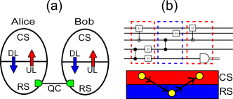
Figure 1: (Color online.) (a): Quantum computation on distributed correlation spaces. Alice who has her own correlation space (CS) downloads (DL) a state from her correlation space to her real physical space (RS), and sends it to Bob through the quantum channel (QC). Bob who receives real physical qubits from Alice uploads (UL) them to his own correlation space for his calculation. (b): The strategy of avoiding less stable space in the virtual-real hybrid QC. The region surrounded by the red (blue) dotted box is the one where the correlation space (real space) is more stable than the other. The yellow circle represents the quantum register. When the correlation (real) space is more stable than the other, the register stays there. Once the space where the register lives becomes less stable than the other, the register emigrates.

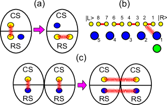
Figure 2: (Color online.) (a): The interpretation of our uploading method in terms of the quantum teleportation. The left of (a): The red zigzag line represents the entanglement-like correlation between the correlation space (CS) and the real space (RS). The right of (a): After the projection measurement in the Bell basis on the two qubits in the real space, the blue state is uploaded (teleported) to the correlation space. The red zigzag line represents the real entanglement. (b): The interpretation of the same uploading method as (a) in terms of the valence-bond (VB) picture RVB . The red zigzag line represents the entanglement-like correlation. The Bell measurement is performed on the first big blue qubit and the big green qubit. The state of the big green qubit is “teleported” to the second yellow small qubit. (c): The entanglement swapping (repeating). The Bell measurement on the two blue qubits in real spaces creates the entanglement between the two yellow qubits in correlation spaces.

Downloading method.— The framework of the computational tensor network Gross starts with the matrix product state $\Phi\big{(}|R\rangle\big{)}_{1}^{N}\equiv\sum_{l_{1},...,l_{N}}\langle L|A[l_{N}]...A[l_{1}]|R\rangle|l_{N},...,l_{1}\rangle$ of $N$ qubits, where $l_{i}\in\{0,1\}$ ($i=1,...,N$), $|L\rangle$ and $|R\rangle$ are two-dimensional complex vectors, $A[0]$ and $A[1]$ are $2\times 2$ complex matrices, and $|l_{i}\rangle$ is the state of $i$th physical qubit in the computational basis $\{|0\rangle,|1\rangle\}$. The quantum computation is performed not in the Hilbert space spanned by $|l_{i}\rangle$’s but in the linear space, which is called the correlation space, where $|L\rangle$, $|R\rangle$, $A[0]$, and $A[1]$ live.

It was shown Cai that a state in the correlation space can be downloaded to the real physical space. Assume that there exists a local basis $\{|m_{0}\rangle,|m_{1}\rangle\}$ such that

$$A[m_{0}]=|\phi_{0}\rangle\langle 0|,~{}~{}A[m_{1}]=|\phi_{1}\rangle\langle 1|$$ (1)

with $\langle\phi_{i}|\phi_{j}\rangle=\delta_{i,j}$, where $A[m_{s}]\equiv\langle m_{s}|0\rangle A[0]+\langle m_{s}|1\rangle A[1]$. Then, by starting with $\Phi(|\psi\rangle)_{1}^{N}$, where $|\psi\rangle$ is the state which we want to download, the method of Ref. Cai gives the state

$$\sum_{s=0}^{1}\Phi(|\phi_{s}\rangle)_{k+1}^{N}\otimes|m_{s}\rangle_{k}\otimes(\tilde{Z}^{s}|\tilde{\psi}\rangle_{1}),$$ (2)

where $\tilde{Z}$ and $|\tilde{\psi}\rangle$ are $Z$ and $|\psi\rangle$ in terms of the $\{|m_{s}\rangle\}$ basis. The projection measurement on the $k$th qubit in the $\{|m_{s}\rangle\}$ basis completes the desired download up to the phase error $\tilde{Z}^{s}$ and the change of the basis $\{|0\rangle,|1\rangle\}\to\{|m_{0}\rangle,|m_{1}\rangle\}$. In general, $A[0]$ and $A[1]$ have more complicated structures than Eq. (1). According to Ref. Gross , the most general form is

$$A[0]\propto W,~{}~{}A[1]\propto W\mbox{diag}(e^{-i\alpha},e^{i\alpha})$$ (3)

for some $W\in SU(2)$. In this case, the filtering Cai $\{\mathcal{F},\bar{\mathcal{F}}\}$ is required in order to make some non-orthogonal physical states orthogonal. The filtering succeeds with a certain probability, and in this case the download succeeds. If the filtering fails, a single physical qubit is consumed. Then, we repeat the filtering on other remaining physical qubits until we succeed.

Uploading method.— Conversely, how to upload a state from a real physical space to the correlation space? One naive way of the upload is to do the inverse of the above downloading method (see Fig. 3 and Appendix 1 and 2). However, it is worth exploring other possibilities since the inverse of the above downloading method has several disadvantages: Firstly, the inverse is complicated even when $A[0]$ and $A[1]$ have the simple form Eq. (1) (see Appendix 1). Secondly, if $A[0]$ and $A[1]$ take the most general form Eq. (3), we must invert the filtering process $\{\mathcal{F},\bar{\mathcal{F}}\}$. Although the inversion of the filtering $\{\mathcal{F},\bar{\mathcal{F}}\}$ is in principle possible by introducing the new filtering $\{\mathcal{G},\bar{\mathcal{G}}\}$ (see Appendix 2), it is cumbersome to prepare two different filterings for the download and the upload. Finally, and most crucially, we must maintain the entanglement between the state $|\psi\rangle$ which we want to upload and the place $\Phi$ where we want to upload during the whole process of the inversion (see Fig. 3): if the entanglement between $|\psi\rangle$ and $\Phi$ is destroyed in the middle of the inversion process, the upload fails and, what is worse, the original state is destroyed (see Appendix 1). This disadvantage makes it difficult to upload a state of, for example, a photon, which is hard to be localized, to the correlation space of stationary qubits, such as atoms, ions, and quantum dots. As we will see later, our uploading method is free from those three disadvantages.

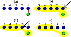
Figure 3: (Color online.) The inverse of the downloading method of Ref. Cai . (a): Blue circles are real physical qubits of $\Phi(|+\rangle)_{1}^{N}$. The green circle is the state $|\psi\rangle$ which we want to upload. The controlled-Z (the red bond) is applied between the first physical qubit in $\Phi(|+\rangle)_{1}^{N}$ and $|\psi\rangle$. (b): The first blue qubit is projected. (c): The second blue qubit is projected. In this way, several blue qubits are projected. (d): Finally, the state of qubits that are not measured (i.e., qubits in the yellow region) is our goal $\Phi(|\psi\rangle)$ where $|\psi\rangle$ is uploaded to the correlation space. Note that if the entanglement between the green qubit and blue qubits is destroyed in the middle of the process, the upload fails.

The other possibility for the way of the upload might be the cloning clone of a state from the real physical space to the correlation space. However, we can see that it is impossible. Assume that we can clone any state $|\psi\rangle$ from the real physical space to the correlation space: $\Phi(|e\rangle)\otimes|\psi\rangle\to\Phi(|\psi\rangle)\otimes|\psi\rangle$, where $|e\rangle$ is a fixed virtual initial state. Then, if we prepare infinitely many $\Phi(|e\rangle)$’s and clone $|\psi\rangle$ to each $\Phi(|e\rangle)$, we have infinitely many $\Phi(|\psi\rangle)$’s, from which we can know the shape of $|\psi\rangle$ without destroying the original. (For a similar reason, the cloning $\Phi(|\psi\rangle)\otimes|e\rangle\to\Phi(|\psi\rangle)\otimes|\psi\rangle$ from the correlation space to the real physical space is also impossible. If it is possible, we can first upload a real physical state $|\psi\rangle$ to the correlation space by using our uploading method which will be explained later, and then repeat the cloning from the correlation space to the real space, which provides an infinitely many copies of $|\psi\rangle$ in the real physical space. Indeed, we can easily verify from Eq. (2) that the downloading method of Ref. Cai destroys the original in the correlation space.)

Since the cloning is impossible, a compromise is the quantum teleportation tele , which regrettably destroys the original state. Indeed, a teleportation-like method of the upload from the real physical space to the correlation space is possible. Let us start with the state $\Phi(|R\rangle)_{1}^{N}\otimes|\psi\rangle_{0}$, where $|\psi\rangle=\lambda_{0}|0\rangle+\lambda_{1}|1\rangle$ is the state which we want to upload and the subscript 0 of $|\psi\rangle_{0}$ indicates that $|\psi\rangle$ is placed on the zeroth site. We can take any state as $|R\rangle$ by running an appropriate pre-processing. By a straightforward calculation, $\Phi(|R\rangle)_{1}^{N}\otimes|\psi\rangle_{0}=\sum_{s,r=0}^{1}\lambda_{r}\Phi(A[m_{s}]|R\rangle)_{2}^{N}\otimes|m_{s}\rangle_{1}\otimes|r\rangle_{0}$, where $\{|m_{0}\rangle,|m_{1}\rangle\}$ is a certain orthonormal basis, and $A[m_{s}]\equiv\langle m_{s}|0\rangle A[0]+\langle m_{s}|1\rangle A[1]$. Let us project the zeroth and first qubits onto $|B_{1}\rangle_{10}\equiv|m_{0}\rangle_{1}\otimes|0\rangle_{0}+|m_{1}\rangle_{1}\otimes|1\rangle_{0}$. Then, we obtain $\Phi(\lambda_{0}A[m_{0}]|R\rangle+\lambda_{1}A[m_{1}]|R\rangle)_{2}^{N}\otimes|B_{1}\rangle_{10}$. If $A[m_{0}]|R\rangle$ and $A[m_{1}]|R\rangle$ are orthogonal with each other, the upload is succeeded up to the trivial change of the basis $\{|0\rangle,|1\rangle\}\to\{A[m_{0}]|R\rangle,A[m_{1}]|R\rangle\}$, which is compensated by a post-processing. For example, the orthogonality between $A[m_{0}]|R\rangle$ and $A[m_{1}]|R\rangle$ is satisfied for the one-dimensional cluster state one-way whose matrix product state is given by Gross $A[0]=|+\rangle\langle 0|$ and $A[1]=|-\rangle\langle 1|$.

It is not difficult to see the strong similarity of the above uploading method to the quantum teleportation tele if we interpret $A[m_{s}]|R\rangle$ (not $\Phi(A[m_{s}]|R\rangle)$!) and $|m_{s}\rangle_{1}$ in

$$\sum_{s=0}^{1}\Phi(A[m_{s}]|R\rangle)_{2}^{N}\otimes|m_{s}\rangle_{1}$$ (4)

as being “entangled” with each other (see Fig. 2 (a) and (b)). Although this entanglement-like correlation is not always connected to the real physical entanglement between the first qubit and other qubits, since the orthogonality of $A[m_{0}]|R\rangle$ and $A[m_{1}]|R\rangle$ does not necessarily mean that of $\Phi(A[m_{0}]|R\rangle)_{2}^{N}$ and $\Phi(A[m_{1}]|R\rangle)_{2}^{N}$ (see Appendix 3), this analogy (and, after all, the mathematical equivalency) between our uploading method and the quantum teleportation is fascinating. For example, the analogy makes it easy to understand what happens if the zeroth and first qubits are projected onto not $|B_{1}\rangle$ but one of other Bell basis $|B_{2}\rangle\equiv|m_{0},0\rangle-|m_{1},1\rangle$, $|B_{3}\rangle\equiv|m_{0},1\rangle+|m_{1},0\rangle$, and $|B_{4}\rangle\equiv|m_{0},1\rangle-|m_{1},0\rangle$ in our uploading method. In this case, as the analogy indicates, the uploaded state is affected by some errors depending on the measurement result. If $A[m_{0}]|R\rangle$ and $A[m_{1}]|R\rangle$ are orthogonal with each other, these errors are the phase error or the bit error in terms of the $\{A[m_{0}]|R\rangle,A[m_{1}]|R\rangle\}$ basis. Such an error is corrected by a post-processing, and therefore the fidelity of the upload is unity. Indeed, if $A[m_{0}]|R\rangle$ and $A[m_{1}]|R\rangle$ are orthogonal with each other, it is reasonable to think that the virtual “entanglement” in Eq. (4) is “maximum”.

If $A[m_{0}]|R\rangle$ and $A[m_{1}]|R\rangle$ are not orthogonal with each other, on the other hand, we are inclined to think that the virtual “entanglement” in Eq. (4) is not “maximum”. Then, the analogy with the quantum teleportation indicates that the upload succeeds only partially. Indeed, it is the case. If $A[m_{0}]|R\rangle$ and $A[m_{1}]|R\rangle$ are not orthogonal with each other, the uploaded state $\lambda_{0}A[m_{0}]|R\rangle+\lambda_{1}A[m_{1}]|R\rangle$ is distorted from the original, and therefore the fidelity of the upload is less than unity. In this case, by applying the same filtering $\{\mathcal{F},\bar{\mathcal{F}}\}$ of Ref. Cai , we can perform a perfect but probabilistic upload. Let us assume that $A[0]$ and $A[1]$ take the most general form Eq. (3). Then, there always exists a basis $\{|m_{0}\rangle,|m_{1}\rangle\}$ such that $A[m_{0}]=r_{0}|\phi_{0}\rangle\langle 0|$ and $A[m_{1}]=r_{1}|\phi_{0}\rangle\langle 0|+|\phi_{1}\rangle\langle 1|$, where $\langle\phi_{i}|\phi_{j}\rangle=\delta_{i,j}$, $r_{0}>0$, $r_{1}\geq 0$, and $r_{0}^{2}+r_{1}^{2}=1$ Cai . By rewriting $\Phi(|+\rangle)_{1}^{N}$ as $\sum_{s=0}^{1}\Phi(|\phi_{s}\rangle)_{2}^{N}\otimes|m_{s}^{\prime}\rangle_{1}$, where $|m_{0}^{\prime}\rangle\equiv r_{0}|m_{0}\rangle+r_{1}|m_{1}\rangle$ and $|m_{1}^{\prime}\rangle\equiv|m_{1}\rangle$, and applying the filtering operation $\{\mathcal{F},\bar{\mathcal{F}}\}$ (for the definition of it, see Appendix 2 or Ref. Cai ) on the first qubit, we probabilistically obtain $\sum_{s=0}^{1}\Phi(|\phi_{s}\rangle)_{2}^{N}\otimes|m_{s}\rangle_{1}$ if $\mathcal{F}$ is realized. In this way, we obtain the state which has the “maximum” entanglement-like correlation between the real physical space and the correlation space. With this state, we can deterministically upload a physical state to the correlation space by using our teleportation-like method explained previously. If the filtering fails (i.e., if $\bar{\mathcal{F}}$ is realized), the net effect of the filtering is the consumption of the first qubit. Therefore, we have only to repeat the same filtering on the remaining qubits until we succeed.

Discussion.— In this letter, we have proposed the teleportation-like method of the upload of a state from a real physical space to the correlation space. Our method is free from the disadvantages of the inverse of the downloading method of Ref. Cai : Firstly, our method is simpler and more intuitive. Secondly, no new filtering is needed for the upload; once the filtering $\{\mathcal{F},\bar{\mathcal{F}}\}$ is prepared, the download is possible with the method of Ref. Cai and the upload is possible with our method. Finally, our method does not require any long-time interaction between the state $|\psi\rangle$ which we want to upload and the place $\Phi$ where we want to upload.

The assumption of the availability of the Bell measurement is, though something to be avoided if possible, not too demanding, since it is ubiquitous in many quantum information protocols, such as the quantum teleportation tele , the quantum dense coding dense , the quantum repeater repeater , and the teleportation-based quantum computation teleQC . In fact, if we want to do the upload, a two-qubit operation is unavoidable: as long as we start with $\Phi(|R\rangle)_{1}^{N}\otimes|\psi\rangle_{0}$, where $|\psi\rangle$ is the state which we want to upload, we must entangle the zeroth qubit with at least one physical qubit in $\Phi(|R\rangle)_{1}^{N}$, since otherwise $\Phi(|R\rangle)_{1}^{N}$ cannot “know” $|\psi\rangle$. Among many possibilities which use two-qubit operations, the teleportation seems to be the most feasible and the most familiar one, since many experimental schemes of the teleportation are available in the optical system, the NMR, the trapped ions, solids, and the light-matter hybrid Furusawa . Note that a universal set of single-qubit rotations, two-qubit entangling gates, and the Deutsch’s algorithm in the correlation space have been recently realized experiment with the four- and six-qubit optical systems. In addition to such an optical system, the systems of bosonic atoms or spin-1 polar molecules trapped in a three-dimensional optical lattice, where the AKLT model is realized through the tunneling-induced collision Yip or the microwave-induced dipole-dipole interaction Brennen , respectively, would be promising places where our uploading method could be implemented, since in the one-dimensional AKLT chain, the right boundary spin-1/2 particle is strongly correlated with the virtual state in the correlation space MiyakeAKLT .

As is easily shown, the teleportation-like method for the download is also possible. However, it will not offer any advantage over the original downloading method of Ref. Cai , since we must implement the Bell measurement in the correlation space, which needs the coupling of two computational quantum wires.

Applications of our uploading method enable several important tricks of quantum information protocols in the virtual-real hybrid setting. For example, we can perform the entanglement swapping between the real spaces and the correlation spaces as is illustrated in Fig. 2 (c) (see Appendix 5). Such a swapping method is useful to establish the entanglement between two correlation spaces without touching them. We can also perform the Gottesman-Chuang gate teleportation trick teleQC from the real space to the correlation space (see Appendix 4); if there are some gates which are difficult to be implemented in the correlation spaces, we can prepare these gates offline in the real spaces and “wedge” them into the correlation spaces as in Ref. KLM . In summary, we believe that our uploading method in addition to the downloading method of Ref. Cai open the door to the new framework of the quantum information processing, namely the virtual-real hybrid quantum information processing.

The author is supported by the ANR (StatQuant, JC07 07205763).

Appendix 1: The inverse of the downloading method of Ref. Cai .— Let us first consider the case of Eq. (1). We start with

$$\Phi(|+\rangle)_{1}^{N}=\sum_{s=0}^{1}\Phi(|\phi_{s}\rangle)_{2}^{N}\otimes|m_{s}\rangle_{1}.$$

Let us couple it with the state

$$|\tilde{\psi}\rangle\equiv\lambda_{0}|m_{0}\rangle+\lambda_{1}|m_{1}\rangle,$$

which is the one we want to upload in terms of the $\{|m_{0}\rangle,|m_{1}\rangle\}$ basis, and apply the controlled-$Z$ gate (in terms of the $\{|m_{0}\rangle,|m_{1}\rangle\}$ basis) between the first qubit and $|\tilde{\psi}\rangle$:

$$\sum_{s=0}^{1}\Phi(|\phi_{s}\rangle)_{2}^{N}\otimes|m_{s}\rangle_{1}\otimes(\tilde{Z}^{s}|\tilde{\psi}\rangle_{0}),$$

where

$$\tilde{Z}\equiv|m_{0}\rangle\langle m_{0}|-|m_{1}\rangle\langle m_{1}|$$

is the Pauli $z$ operator in terms of the $\{|m_{0}\rangle,|m_{1}\rangle\}$ basis, and $|\tilde{\psi\rangle}$ is placed on the zeroth site. It is rewritten as

$$\lambda_{0}\Phi(|+\rangle)_{1}^{N}\otimes|m_{0}\rangle_{0}+\lambda_{1}\Phi(|-\rangle)_{1}^{N}\otimes|m_{1}\rangle_{0}.$$

Note that if the zeroth site is measured in the $\{|m_{0}\rangle,|m_{1}\rangle\}$ basis at this stage, the entanglement between the zeroth site and other sites is destroyed, and therefore the information about $\{\lambda_{0},\lambda_{1}\}$ is lost. Then, the upload fails.

By implementing the rotation $\{|+\rangle,|-\rangle\}\to\{|\phi_{0}\rangle,|\phi_{1}\rangle\}$ in the correlation space, which is always possible by the definition of the computational quantum wire, we obtain

$$\lambda_{0}\Phi(|\phi_{0}\rangle)_{k}^{N}\otimes|m_{0}\rangle_{0}+\lambda_{1}\Phi(|\phi_{1}\rangle)_{k}^{N}\otimes|m_{1}\rangle_{0}$$

for certain $k$. Again, if the entanglement between the zeroth site and other sites is destroyed at this stage, the upload fails. It is rewritten as

$$\sum_{s=0}^{1}\Phi(A[m_{s}]|\psi\rangle)_{k}^{N}\otimes|m_{s}\rangle_{0}.$$

By changing the basis of the zeroth site to the computational basis, and swapping the zeroth site with the $k-1$th site, we obtain $\Phi(|\psi\rangle)_{k-1}^{N}$, which is our goal. Note that the original state (zeroth site) is interacting with $\Phi$ from the beginning to the end.

Appendix 2: Filtering.— Let us next consider the case of Eq. (3). In this case, there always exists a basis $\{|m_{0}\rangle,|m_{1}\rangle\}$ such that

$$A[m_{0}]=r_{0}|\phi_{0}\rangle\langle 0|,~{}~{}A[m_{1}]=r_{1}|\phi_{0}\rangle\langle 0|+|\phi_{1}\rangle\langle 1|,$$

where $\langle\phi_{i}|\phi_{j}\rangle=\delta_{i,j}$, $r_{0}>0$, $r_{1}\geq 0$, and $r_{0}^{2}+r_{1}^{2}=1$ Cai . Let us define

$$|m_{0}^{\prime}\rangle \equiv r_{0}|m_{0}\rangle+r_{1}|m_{1}\rangle$$

$$|m_{1}^{\prime}\rangle \equiv |m_{1}\rangle.$$

In principle, the download for the case of Eq. (3) is performed in a similar way as that for the case of Eq. (1). However, in the case of Eq. (3), the filtering Cai $\{\mathcal{F},\bar{\mathcal{F}}\}$ is required in order to transform non-orthogonal states $\{|m_{0}^{\prime}\rangle,|m_{1}^{\prime}\rangle\}$ into orthogonal states $\{|m_{0}\rangle,|m_{1}\rangle\}$. Here,

$$\mathcal{F}^{\dagger}\mathcal{F}+\bar{\mathcal{F}}^{\dagger}\bar{\mathcal{F}}=I,$$

$$\mathcal{F} \equiv \frac{1}{\sqrt{1+r_{1}}}\Big{(}|m_{0}\rangle\langle m_{0}|+r_{0}|m_{1}\rangle\langle m_{1}|-r_{1}|m_{1}\rangle\langle m_{0}|\Big{)},$$

$$\bar{\mathcal{F}} \equiv \sqrt{\frac{2r_{1}}{1+r_{1}}}|\xi\rangle\langle\xi|,$$

and

$$|\xi\rangle\equiv\sqrt{\frac{1-r_{1}}{2}}|m_{0}\rangle+\sqrt{\frac{1+r_{1}}{2}}|m_{1}\rangle.$$

Let us consider how to invert the downloading method of Ref. Cai when the filtering is required. We start with

$$\Phi(|+\rangle)_{1}^{N}=\sum_{s=0}^{1}\Phi(|\phi_{s}\rangle)_{2}^{N}\otimes|m_{s}^{\prime}\rangle_{1}.$$

By using the filtering $\{\mathcal{F},\bar{\mathcal{F}}\}$, we can do the transformation $\{|m_{0}^{\prime}\rangle,|m_{1}^{\prime}\rangle\}\to\{|m_{0}\rangle,|m_{1}\rangle\}$:

$$\sum_{s=0}^{1}\Phi(|\phi_{s}\rangle)_{2}^{N}\otimes|m_{s}\rangle_{1}.$$

Let us implement the controlled-Z gate (in terms of the $\{|m_{0}\rangle,|m_{1}\rangle\}$ basis) between the first qubit and

$$|\tilde{\psi}\rangle\equiv\lambda_{0}|m_{0}\rangle+\lambda_{1}|m_{1}\rangle,$$

which is the state we want to upload in terms of the $\{|m_{0}\rangle,|m_{1}\rangle\}$ basis. Then, we obtain

$$\sum_{s=0}^{1}\Phi(|\phi_{s}\rangle)_{2}^{N}\otimes|m_{s}\rangle_{1}\otimes(\tilde{Z}^{s}|\tilde{\psi}\rangle_{0}),$$

where $|\psi\rangle$ is placed on the zeroth site, and $\tilde{Z}$ is $Z$ in terms of the $\{|m_{0}\rangle,|m_{1}\rangle\}$ basis. If we can do the transformation $\{|m_{0}\rangle,|m_{1}\rangle\}\to\{|m_{0}^{\prime}\rangle,|m_{1}^{\prime}\rangle\}$, we obtain

$$\sum_{s=0}^{1}\Phi(|\phi_{s}\rangle)_{2}^{N}\otimes|m_{s}^{\prime}\rangle_{1}\otimes(\tilde{Z}^{s}|\tilde{\psi}\rangle_{0}).$$

By a streightforward calculation, it is equivalent to

$$\lambda_{0}\Phi(|+\rangle)_{1}^{N}\otimes|m_{0}\rangle_{0}+\lambda_{1}\Phi(|-\rangle)_{1}^{N}\otimes|m_{1}\rangle_{0}.$$

By implementing the rotation $\{|+\rangle,|-\rangle\}\to\{|\phi_{0}\rangle,|\phi_{1}\rangle\}$ in the correlation space, which is alway possible if $N$ is sufficiently large, we obtain

$$\sum_{s=0}^{1}\lambda_{s}\Phi(|\phi_{s}\rangle)_{k}^{N}\otimes|m_{s}\rangle_{0}$$

for certain $k$. By using the filtering $\{|m_{s}\rangle\}\to\{|m_{s}^{\prime}\rangle\}$, we obtain

$$\sum_{s=0}^{1}\lambda_{s}\Phi(|\phi_{s}\rangle)_{k}^{N}\otimes|m_{s}^{\prime}\rangle_{0}=\Phi(|\psi\rangle),$$

which is our goal.

The operation $\{|m_{0}\rangle,|m_{1}\rangle\}\to\{|m_{0}^{\prime}\rangle,|m_{1}^{\prime}\rangle\}$ is possible, for example, with the filtering $\{\mathcal{G},\bar{\mathcal{G}}\}$, where

$$\mathcal{G}^{\dagger}\mathcal{G}+\bar{\mathcal{G}}^{\dagger}\bar{\mathcal{G}}=I,$$

$$\mathcal{G} \equiv \frac{1}{\sqrt{1+r_{1}}}\Big{(}r_{0}|m_{0}\rangle\langle m_{0}|+r_{1}|m_{1}\rangle\langle m_{0}|+|m_{1}\rangle\langle m_{1}|\Big{)}$$

$$\bar{\mathcal{G}} \equiv \sqrt{\frac{2r_{1}}{1+r_{1}}}|\eta\rangle\langle\eta|,$$

and

$$|\eta\rangle\equiv\frac{1}{\sqrt{2}}(|m_{0}\rangle-|m_{1}\rangle).$$

Appendix 3: Calculation of the inner product.— Let us calculate the inner product between $\Phi(|+\rangle)_{1}^{N}$ and $\Phi(|-\rangle)_{1}^{N}$ with $A[0]=|\phi_{0}\rangle\langle 0|$, $A[1]=|\phi_{1}\rangle\langle 1|$, and $|L\rangle=|0\rangle$, where

$$|\phi_{0}\rangle \equiv \cos\frac{\theta}{2}|0\rangle+\sin\frac{\theta}{2}|1\rangle$$

$$|\phi_{1}\rangle \equiv \sin\frac{\theta}{2}|0\rangle-\cos\frac{\theta}{2}|1\rangle.$$

By the contraction, the inner product is

$$\sum_{l_{N},...,l_{1}=0}^{1}\langle-|A[l_{1}]^{\dagger}...A[l_{N}]^{\dagger}|0\rangle\langle 0|A[l_{N}]...A[l_{1}]|+\rangle,$$

which is interpreted as

$$\langle-|\Big{[}\mathcal{E}\circ...\circ\mathcal{E}(|0\rangle\langle 0|)\Big{]}|+\rangle$$

with the map

$$\mathcal{E}(\rho)\equiv\sum_{s=0}^{1}A[s]^{\dagger}\rho A[s],$$

which works as

$$\mathcal{E}(|0\rangle\langle 0|) = \cos^{2}\frac{\theta}{2}|0\rangle\langle 0|+\sin^{2}\frac{\theta}{2}|1\rangle\langle 1|$$

$$\mathcal{E}(|1\rangle\langle 1|) = \sin^{2}\frac{\theta}{2}|0\rangle\langle 0|+\cos^{2}\frac{\theta}{2}|1\rangle\langle 1|.$$

Under the correspondence

$$|0\rangle\langle 0| \iff \left(\begin{matrix}1\\ 0\end{matrix}\right)$$

$$|1\rangle\langle 1| \iff \left(\begin{matrix}0\\ 1\end{matrix}\right),$$

the map $\mathcal{E}$ works as

$$\mathcal{E}=\left(\begin{matrix}\cos^{2}\frac{\theta}{2}&\sin^{2}\frac{\theta}{2}\\ \sin^{2}\frac{\theta}{2}&\cos^{2}\frac{\theta}{2}.\end{matrix}\right).$$

Since this $2\times 2$ matrix is diagonalized by the unitary

$$\frac{1}{\sqrt{2}}\left(\begin{matrix}1&1\\ 1&-1\end{matrix}\right)$$

as diag($1,\cos\theta$), we obtain

$$\langle-|\Big{[}\mathcal{E}\circ...\circ\mathcal{E}(|0\rangle\langle 0|)\Big{]}|+\rangle=\frac{1}{2}\cos^{N}\theta.$$

Since the norm of $\Phi(|+\rangle)_{1}^{N}$ and $\Phi(|-\rangle)_{1}^{N}$ is $\frac{1}{\sqrt{2}}$, the normalized inner product is $\cos^{N}\theta$.

Appendix 4: Gate teleportation.— Let us first consider the teleportation of a single-qubit unitary teleQC . Without loss of generality, we can start with

$$\sum_{s=0}^{1}\Phi(|\phi_{s}\rangle)_{2}^{N}\otimes|m_{s}\rangle_{1},$$

since if $A[0]$ and $A[1]$ have the form Eq. (1), we immediately obtain this state, and if $A[0]$ and $A[1]$ have the form Eq. (3), we obtain this state by using the filtering. By the definition of the computational quantum wire, the basis change $\{|\phi_{0}\rangle,|\phi_{1}\rangle\}\to\{|0\rangle,|1\rangle\}$ is always possible:

$$\sum_{s=0}^{1}\Phi(|s\rangle)_{k}^{N}\otimes|m_{s}\rangle_{1}$$

for certain $k$. Then, by projecting the zeroth and first qubit of

$$\Big{[}\sum_{s=0}^{1}\Phi(|s\rangle)_{k}^{N}\otimes|m_{s}\rangle_{1}\Big{]}\otimes|\psi\rangle_{0}$$

onto $(I_{1}\otimes U^{\dagger}_{0})|B\rangle_{10}$, where $I_{1}$ is the identity operator on the first qubit, $U_{0}$ is a unitary on the zeroth qubit, and $|B\rangle_{10}$ is one of the Bell basis

$$|m_{0}\rangle_{1}\otimes|0\rangle_{0}+|m_{1}\rangle_{1}\otimes|1\rangle_{0},$$

$$|m_{0}\rangle_{1}\otimes|0\rangle_{0}-|m_{1}\rangle_{1}\otimes|1\rangle_{0},$$

$$|m_{0}\rangle_{1}\otimes|1\rangle_{0}+|m_{1}\rangle_{1}\otimes|0\rangle_{0},$$

$$|m_{0}\rangle_{1}\otimes|1\rangle_{0}-|m_{1}\rangle_{1}\otimes|0\rangle_{0},$$

we obtain the desired state $\Phi(U|\psi\rangle)$ up to the bit or phase errors in the correlation space.

Next, let us consider the teleportation of the controlled-Z gate teleQC ; RVB

$$|0\rangle\langle 0|\otimes I+|1\rangle\langle 1|\otimes Z.$$

Without loss of generality, we can start with the state (see Fig. 4)

$$\Big{[}\sum_{s=0}^{1}\Phi(|\phi_{s}\rangle_{6})\otimes|m_{s}\rangle_{5}\Big{]}\otimes\Big{[}\sum_{r=0}^{1}\Phi(|\phi_{r}\rangle_{8})\otimes|m_{r}\rangle_{7}\Big{]}$$

$$\otimes|B\rangle_{34}\otimes|\psi\rangle_{12},$$

where

$$|\psi\rangle_{12} = c_{00}|0\rangle_{1}\otimes|0\rangle_{2}+c_{01}|0\rangle_{1}\otimes|1\rangle_{2}$$

$$+c_{10}|1\rangle_{1}\otimes|0\rangle_{2}+c_{11}|1\rangle_{1}\otimes|1\rangle_{2}$$

is the state of the first and second qubits, and

$$|B\rangle_{34}\equiv|0\rangle_{3}\otimes|0\rangle_{4}+|1\rangle_{3}\otimes|1\rangle_{4}$$

is the maximally entangled state of the third and fourth qubits. The first, third, and fifth qubits are projected onto

$$|0\rangle_{1}\otimes|0\rangle_{3}\otimes|m_{0}\rangle_{5}+|1\rangle_{1}\otimes|1\rangle_{3}\otimes|m_{1}\rangle_{5},$$

whereas the second, fourth, and seventh qubits are projected onto

$$|0\rangle_{2}\otimes|+\rangle_{4}\otimes|m_{0}\rangle_{7}+|1\rangle_{2}\otimes|-\rangle_{4}\otimes|m_{1}\rangle_{7}.$$

Then, we obtain the desired state

$$c_{00}\Phi(|\phi_{0}\rangle_{6})\otimes\Phi(|\phi_{0}\rangle_{8})+c_{01}\Phi(|\phi_{0}\rangle_{6})\otimes\Phi(|\phi_{1}\rangle_{8})$$

$$+c_{10}\Phi(|\phi_{1}\rangle_{6})\otimes\Phi(|\phi_{0}\rangle_{8})-c_{11}\Phi(|\phi_{1}\rangle_{6})\otimes\Phi(|\phi_{1}\rangle_{8}).$$

We obtain the same result up to the trivial errors if the six qubits are projected onto other states.

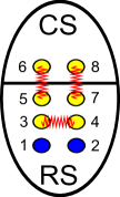
Figure 4: (Color online.) Teleportation of the controlled-Z gate from the real space to the correlation space. Two blue circles represent the two-qubit state $|\psi\rangle$. The Red zigzag line between the third and fourth qubits represents the real physical entanglement. Other red zigzag lines represent the virtual ”entanglement”. The first, third, and fifth qubits are projected. The second, fourth, and seventh qubits are projected. Then, the state of the sixth and eighth qubits is $CZ|\psi\rangle$ up to some trivial errors.

Appendix 5: Entanglement swapping.— Let us see Fig. 2 (c). The initial state is

$$\Big{[}\sum_{s=0}^{1}\Phi(|\phi_{s}\rangle)\otimes|m_{s}\rangle\Big{]}\otimes\Big{[}\sum_{r=0}^{1}\Phi(|\phi_{r}\rangle)\otimes|m_{r}\rangle\Big{]}.$$

Two real physical qubits are projected onto one of the Bell basis

$$|m_{0}\rangle\otimes|m_{0}\rangle+|m_{1}\rangle\otimes|m_{1}\rangle$$

$$|m_{0}\rangle\otimes|m_{0}\rangle-|m_{1}\rangle\otimes|m_{1}\rangle$$

$$|m_{0}\rangle\otimes|m_{1}\rangle+|m_{1}\rangle\otimes|m_{0}\rangle$$

$$|m_{0}\rangle\otimes|m_{1}\rangle-|m_{1}\rangle\otimes|m_{0}\rangle.$$

Then, we obtain the desired state

$$\sum_{s=0}^{1}\Phi(|\phi_{s}\rangle)\otimes\Phi(|\phi_{s}\rangle)$$

up to the phase or the bit errors.

References

• (1) R. Raussendorf and H. J. Briegel, Phys. Rev. Lett. 86, 5188 (2001).
• (2) D. Gross and J. Eisert, Phys. Rev. Lett. 98, 220503 (2007).
• (3) J. M. Cai, et. al., Phys. Rev. Lett. 103, 050503 (2009).
• (4) M. Van den Nest, et. al., Phys. Rev. Lett. 97, 150504 (2006).
• (5) D. Gottesman and I. L. Chuang, Nature 402, 390 (1999).
• (6) F. Verstraete and J. I. Cirac, Phys. Rev. A 70, 060302(R) (2004).
• (7) W. K. Wootters and W. H. Zurek, Nature 299, 802 (1982).
• (8) C. H. Bennett, et. al., Phys. Rev. Lett. 70, 1895 (1993).
• (9) C. H. Bennett and S. J. Wiesner, Phys. Rev. Lett. 69, 2881 (1992).
• (10) H. J. Briegel, et. al., Phys. Rev. Lett. 81, 5932 (1998).
• (11) F. Furusawa, et. al., Science 282, 706 (1998); M. A. Nielsen, et. al., Nature 396, 52 (1998); M. Riebe, et. al., Nature 429, 734 (2004); M. D. Barrett, et. al., Nature 429, 737 (2004); J. H. Reina and N. F. Johnson, Phys. Rev. A 63, 012303 (2000); J. Sherson, et. al., Nature 443, 557 (2006); Y. A. Chen, et. al., Nature Physics 4, 103 (2008).
• (12) W. B. Gao, et. al., arXiv:1004.4162.
• (13) S. K. Yip, Phys. Rev. Lett. 90, 250402 (2003).
• (14) G. K. Brennen, et. al., New J. Phys. 9, 138 (2007).
• (15) G. K. Brennen and A. Miyake, Phys. Rev. Lett. 101, 010502 (2008).
• (16) E. Knill, et. al., Nature 46, 409 (2001).