A Repeated Game Formulation of Energy-Efficient Decentralized Power Control

Abstract

Decentralized multiple access channels where each transmitter wants to selfishly maximize his transmission energy-efficiency are considered. Transmitters are assumed to choose freely their power control policy and interact (through multiuser interference) several times. It is shown that the corresponding conflict of interest can have a predictable outcome, namely a finitely or discounted repeated game equilibrium. Remarkably, it is shown that this equilibrium is Pareto-efficient under reasonable sufficient conditions and the corresponding decentralized power control policies can be implemented under realistic information assumptions: only individual channel state information and a public signal are required to implement the equilibrium strategies. Explicit equilibrium conditions are derived in terms of minimum number of game stages or maximum discount factor. Both analytical and simulation results are provided to compare the performance of the proposed power control policies with those already existing and exploiting the same information assumptions namely, those derived for the one-shot and Stackelberg games.

I Introduction

Many current wireless communications systems (e.g., cellular networks) are optimized in terms of quality of service (QoS), which can include for example, performance criteria such as transmission rate, reliability, latency, or security. It turns out that applications where trade-offs have to be found between QoS and energy consumptions, have become more and more important, especially over the past decade. Wireless sensor networks and ad-hoc networks are two good examples illustrating the importance of finding such trade-offs. A very simple and pragmatic way of knowing to what extent a communication is energy-efficient has been proposed by [1][2]. The authors of [1][2] define energy-efficiency as the net number of information bits that are transmitted without error per unit time (goodput) to the transmit power level. More specifically, the authors analyze the problem of distributed power control (PC) in flat fading multiple access channels (MACs). The problem is formulated as a non-cooperative game where the players are the transmitters, the action of a given player is her/his/its transmit power (“his” is chosen in this paper), and his payoff/reward/utility function is the energy-efficiency of his communication with the receiver. The results reported in [1][2] have been extended to the case of multi-carrier systems in [3]. Unfortunately, as shown in [2], Nash equilibria (NE) resulting from the one-shot game formulation of the energy-efficient power control problem are generally inefficient. This is one of the reasons why some authors proposed to apply other game-theoretic concepts to improve efficiency of the network equilibrium: [4] proposed a pricing mechanism and [5] proposed to introduce some hierarchy in the network by considering a Stackelberg game [6] or using successive interference cancellation at the receiver. The solution of [4] has the advantage to be Pareto-optimal (PO) but requires global channel state information (CSI) at the transmitters and equilibrium uniqueness is not proven analytically. On the other hand, the solution of [5] is not PO but only requires individual CSI and uniqueness is guaranteed.

All the cited and related works on energy-efficient PC ([3][4][5], etc) have at least one common point: time is divided into windows or blocks over which the channel is assumed to be constant and transmit power levels can be updated only once within a given block. The corresponding framework is the one of static or one-shot games which is to say, transmitters play independently from block to block and maximize their instantaneous utility for each block. In this paper, we consider a more general situation: transmitters are allowed to update their power levels several times within a block; the corresponding PC type could be called decentralized fast PC (DFPC), generalizing the more conventional decentralized slow PC (DSPC) for which the power can be updated only once per block. Both in the DFPC and DSPC cases, we want to take into account the fact that players (namely the transmitters) interact several times within a block or/and from block to block, which introduces new types of behaviors (cooperation, punishment, etc) with respect to the one-shot game. The framework considered here is the one of dynamic games. More specifically, we analyze a special case of dynamic games, which is the case of repeated games (RG). In standard repeated games [7][8][9] the same game is played a finite or infinite number of times and players are interested in optimizing a certain performance metric, resulting from averaging their utility over the whole duration of the game. In contrast with iterative or learning techniques that are based on mild information assumptions and different behavior assumptions (transmitters can be modeled by automata), RG generally require more demanding information and behavior assumptions. Also, RG aim at optimizing an averaged utility and reaching points more efficient than the one-shot game NE. Two important models of RG are considered: the finitely repeated game (FRG) [10] and discounted repeated game (DRG) [11]. A priori, the FRG seems to be more suited to DFPC since the number of times players interact is finite and can be known (e.g., the number of training symbols in a block) whereas the DRG seems to be more suited to DSPC with a uncertain number of blocks over which players interact. To the authors’ knowledge, there is only a small fraction of papers dedicated to repeated games in the wireless literature. As far as the present paper is concerned, the most relevant contributions available are [12][13][14]. With respect to these works, our contributions are as follows. The work reported in this paper is the first to apply the concept of RG to energy-efficient PC (the existing works consider Shannon transmission rates or similar utility functions). A second important feature of the present analysis is that only individual CSI and signal-to-interference plus noise ratio (SINR) are needed to implement the proposed PC scheme, which is not the case in [12][13][14]. Third, two models of RG are considered and explicit equilibrium conditions on the number of game stages (for the FRG) and discounted factor (for the DRG) are provided and discussed, which is not made in the existing literature. At last but not least, the PC policy we propose is compared in a fair manner with existing game-theoretic PC policies both analytically and by simulations and shown to be the most efficient one (in the sense of Pareto). For this purpose, several works from the game theory literature, and not used yet by the wireless community, are exploited.

This paper is structured as follows. In Sec. II-A the assumed signal model is described. This is followed (Sec. II-B) by a short review of the static/one-shot non-cooperative and Stackelberg PC games. In Sec. III a rigorous RG formulation of the PC problem is provided and information assumptions necessary to implement the equilibrium strategies of Sec. IV-B are given. The proposed equilibria (finitely and discounted repeated games equilibria) and their properties are analyzed in Sec. IV. The results derived are illustrated by simulations in Sec. V, which is followed by the conclusion (Sec. VI).

II System model

II-A Signal model

We consider a decentralized MAC with a finite number of transmitters, which is denoted by $K$. The network is said to be decentralized in the sense that the receiver (e.g., a base station) does not dictate to the transmitters (e.g., mobile stations) their PC policy. Rather, all the transmitters choose their policy by themselves and want to selfishly maximize their energy-efficiency; in particular, they can ignore some specified centralized policies. We assume that the users transmit their data over quasi-static channels and at the same time and frequency band. Note that a block is defined as a sequence of $M$ consecutive symbols which comprises a training sequence that is, a certain number of consecutive symbols used to estimate the channel (or other related quantities) associated with a given block. A block has therefore a duration less than the channel coherence time. The signal model used corresponds to the information-theoretic channel model used for studying MAC [15][16]; see e.g., [17] for more comments on the multiple access technique involved. What matters is that this model is both simple to be presented and captures the different aspects of the problem (the SINR structure in particular) and can be readily applied to speficic systems such as CDMA systems [2][5] or multi-carrier CDMA systems [3]. The equivalent baseband signal received by the base station can be written as

$$y(n)=\sum_{i=1}^{K}g_{i}(n)x_{i}(n)+z(n)$$ (1)

where $i\in\mathcal{K}$, $\mathcal{K}=\{1,...,K\}$, $x_{i}(n)$ represents the symbol transmitted by transmitter $i$ at time $n$, $\mathbb{E}|x_{i}|^{2}=p_{i}$, the noise $z$ is assumed to be distributed according to a zero-mean Gaussian random variable with variance $\sigma^{2}$ and each channel gain $g_{i}$ varies over time but is assumed to be constant over each block. For each transmitter $i$, the channel gain modulus is assumed to lie in a compact set $\left|g_{i}\right|^{2}\in\left[\eta_{i}^{\mathrm{min}},\eta_{i}^{\mathrm{max}}\right]$. This assumption is both practical (for example, such limitations can model the finite receiver sensitivity and the existence of a minimum distance between the transmitter and receiver) and important to guarantee the existence of the proposed equilibria (Sec. IV). At last, the receiver is assumed to implement single-user decoding.

II-B Review of the one-shot power control game

Here, we review a few key results from [2] concerning the static non-cooperative PC game. In order to define the static PC game some notations need to be introduced. We denote by $R_{i}$ the transmission information rate (in bps) for user $i$ and $f$ an efficiency function representing the block success rate, which is assumed to be sigmoidal and identical for all the users; the sigmoidness assumption is a reasonable assumption, which is well justified in [18][19]. Recently, [20] has shown that this assumption is also justified from an information-theoretic standpoint. At a given instant, the SINR at receiver $i\in\mathcal{K}$ writes as:

$$\mathrm{SINR}_{i}=\frac{p_{i}|g_{i}|^{2}}{\sum_{j\neq i}p_{j}|g_{j}|^{2}+\sigma^{2}}$$ (2)

where $p_{i}$ is the power level for transmitter $i$. With these notations, the static PC game, called $\mathcal{G}$, is defined in its normal form as follows.

Definition 1 (Static PC game)

The static PC game is a triplet $\mathcal{G}=(\mathcal{K},\{\mathcal{A}_{i}\}_{i\in\mathcal{K}},\{u_{i}\}_{i\in\mathcal{K}})$ where $\mathcal{K}$ is the set of players, $\mathcal{A}_{1},...,\mathcal{A}_{K}$ are the corresponding sets of actions, $\mathcal{A}_{i}=[0,P_{i}^{\mathrm{max}}]$, $P_{i}^{\mathrm{max}}$ is the maximum transmit power for player $i$, and $u_{1},...,u_{k}$ are the utilities of the different players which are defined by:

$$u_{i}(p_{1},...,p_{K})=\frac{R_{i}f(\mathrm{SINR}_{i})}{p_{i}}\ [\mathrm{bit}/\mathrm{J}].$$ (3)

In this game with complete information ($\mathcal{G}$ is known to every player) and rational players (every player does the best for himself and knows the others do so and so on), an important game solution concept is the NE (i.e., a point from which no player has interest in unilaterally deviating). When it exists, the non-saturated NE of this game can by obtained by setting $\frac{\partial u_{i}}{\partial p_{i}}$ to zero, which gives an equivalent condition on the SINR: the best SINR in terms of energy-efficiency for transmitter $i$ has to be a solution of $xf^{\prime}(x)-f(x)=0$ (this solution is independent of the player index since a common efficiency function is assumed, see [19] for more details). This leads to:

$$\forall i\in\{1,...,K\},\ p_{i}^{*}=\frac{\sigma^{2}}{|g_{i}|^{2}}\frac{\beta^{*}}{1-(K-1)\beta^{*}}$$ (4)

where $\beta^{*}$ is the unique solution of the equation $xf^{\prime}(x)-f(x)=0$. By using the term “non-saturated NE” we mean that the maximum transmit power for each user, denoted by $P_{i}^{\mathrm{max}}$, is assumed to be sufficiently high not to be reached at the equilibrium i.e., each user maximizes his energy-efficiency for a value less than $P_{i}^{\mathrm{max}}$ (see [5] for more details). An important property of the NE given by (4) is that transmitters only need to know their individual channel gain $|g_{i}|$ to play their equilibrium strategy. One of the interesting results of this paper is that it is possible to obtain a more efficient equilibrium point by repeating the game $\mathcal{G}$ while keeping this key property.

II-C Review of the Stackelberg power control game

Here we review a few key results from [5]. The corresponding results will be used in Sec. IV and V where the performance of the proposed RG equilibrium is compared with the one of the Stackelberg equilibrium (SE). The main difference between the one-shot game [2] and the Stackelberg game is that in the latter, one of the transmitters is the leader of the game. The other transmitters are assumed to be able to observe the actions of the leader and react to them accordingly; these transmitters are called the followers. Note that the leader knows that his actions are observed and therefore anticipates the reaction of the followers. In [5], it is shown that the SE power profile Pareto-dominates the one-shot NE power profile. The power played by transmitter $i\in\mathcal{K}$ at the SE when he is the game leader (L) is given by: $p_{i}^{L}=\frac{\sigma^{2}}{|g_{i}|^{2}}\frac{\gamma^{*}(1+\beta^{*})}{1-(K-1)\gamma^{*}\beta^{*}-(K-2)\beta^{*}}$ where $\gamma^{*}$ is the unique solution of $x\left[1-\frac{(K-1)\beta^{*}}{1-(K-2)\beta^{*}}x\right]f^{\prime}(x)-f(x)=0$, and the corresponding utility is $u^{L}_{i}=\frac{|g_{i}|^{2}}{\sigma^{2}}\frac{1-(K-1)\gamma^{*}\beta^{*}-(K-2)\beta^{*}}{\gamma^{*}(1+\beta^{*})}f(\gamma^{*})$. On the other hand, the power played by transmitter $i\in\mathcal{K}$ at the SE when he is one of the game followers (F) and corresponding utility are given by $p_{i}^{F}=\frac{\sigma^{2}}{|g_{i}|^{2}}\frac{\beta^{*}(1+\gamma^{*})}{1-(K-1)\gamma^{*}\beta^{*}-(K-2)\beta^{*}}$ and $u^{F}_{i}=\frac{|g_{i}|^{2}}{\sigma^{2}}\frac{1-(K-1)\gamma^{*}\beta^{*}-(K-2)\beta^{*}}{\beta^{*}(1+\gamma^{*})}f(\beta^{*})$.

III Moving from static to repeated PC games

III-A Strategic information assumptions

First, we want to show that, in the non-saturated regime (as defined in the preceding section), the energy-efficient one-shot PC game has a very interesting structure in terms of CSI. This structure, which is analyzed just below, has two consequences. The first consequence is that only individual CSI is required at the transmitters that is, only $|g_{i}|$ needs to be known by transmitter $i$. In the existing literature ([2][3][5], etc) this game feature is observed once the equilibrium solution has been determined. It turns out that it is due to the structure of the utility functions of the one-shot game and not only to the specific solutions analyzed in the existing literature. This can therefore be checked before deriving the equilibrium solution. A simple way of proving this statement is to consider a game where utilities are normalized: $\frac{u_{i}(p_{1},...,p_{K})}{|g_{i}|^{2}}=\frac{R_{i}f\left(\frac{p_{i}|g_{i}|^{2}}{\sum_{j\not=i}p_{j}|g_{j}|^{2}+\sigma^{2}}\right)}{p_{i}|g_{i}|^{2}}$. By making the change of variables $a_{i}=p_{i}|g_{i}|^{2}$ the normalized utility function becomes: $\hat{u}_{i}(a_{1},...,a_{K})=\frac{R_{i}f\left(\frac{a_{i}}{\sum_{j\not=i}a_{j}+\sigma^{2}}\right)}{a_{i}}$. It is seen from the normalized utilities that channel gains play only a role when players de-normalize their actions by computing $p_{i}=\frac{a_{i}}{|g_{i}|^{2}}$, which shows that only individual CSI is needed to play the game. The second consequence of the structure of $\hat{u}_{i}$ is that the repeated versions of the one-shot game are easier to be analyzed. Indeed, the normalized utilities $\hat{u}_{i}$ depend on time only through the action profile $\underline{a}=(a_{1},...,a_{K})$ and not through $|g_{i}|$. This means that the PC stochastic repeated game can be analyzed as the repeated version of a (normalized) static game; this is why, in the sequel, we will not use a time index for $u_{i}$. In addition to the individual CSI assumption, we also assume that every player can observe a public signal. More specifically, we assume that every player knows at each stage of the game the signal

$$\omega=\sigma^{2}+\sum_{i=1}^{K}|g_{i}|^{2}p_{i}.$$ (5)

By noticing that $\forall i\in\mathcal{K},\ p_{i}|g_{i}|^{2}\times\frac{\mathrm{SINR}_{i}+1}{\mathrm{SINR}_{i}}=\omega$ we see that each transmitter can construct the public signal from the sole knowledge of his action, individual channel gain, and individual SINR. One of the main results of this paper is that assuming the two mentioned information assumptions allows one to implement a cooperation plan between the transmitters corresponding to an efficient equilibrium. This is possible with the repeated game formulation of the problem, which is given below.

III-B Repeated game formulation of the power control problem

In the static PC game, each transmitter observes the channel gain associated with the current block i.e., $|g_{i}|$ and updates his power level according to (4) in order to maximize his instantaneous utility. In repeated games, players want to maximize their averaged utility. To define the latter quantity we first need to define several notions namely a game stage, the game history, and the strategy of a player. Game stages correspond to instants at which players can choose their actions. To be concrete, in the case of DSPC, game stages coincide with blocks whereas in the case of DFPC, game stages coincide with sub-blocks (comprising one or several symbols). The proposed framework is the one of repeated games with a public signal (see e.g., [22][23]) in which the public signal (namely (5)) is a deterministic function of the played actions. We denote by $\Omega=\displaystyle{\left[\sigma^{2},\sigma^{2}+\sum_{i=1}^{K}\eta_{i}^{\max}P_{i}^{\mathrm{max}}\right]}$ the interval the public signal lies in. The pair of vectors $(\underline{\omega}_{t},\underline{p}_{i,t})=\left(\omega(1),...,\omega(t-1),p_{i}(1),...,p_{i}(t-1)\right)$ is called the history of the game for transmitter $i$ at time $t$ and lies in the set $\mathcal{H}_{t}=\Omega^{t-1}\times\mathcal{P}_{i}^{t-1}$. This is precisely the history $\underline{h}_{t}=\left(\underline{\omega}_{t},\underline{p}_{i,t}\right)$ which is assumed to be known by the transmitters before playing at stage $t$. With these notations, a pure strategy of a transmitter in the repeated game can be defined properly.

Definition 2 (Players’ strategies in the RG)

A pure strategy $\tau_{i}$ for player $i\in\mathcal{K}$ is a sequence of causal functions $\left(\tau_{i,t}\right)_{t\geq 1}$ with

$$\tau_{i,t}:\left|\begin{array}[]{ccc}\mathcal{H}_{t}&\rightarrow&[0,P_{i}^{\mathrm{max}}]\\ \underline{h}_{t}&\mapsto&p_{i}(t).\end{array}\right.$$ (6)

The strategy of player $i$, which is a sequence of functions, will be denoted by $\tau_{i}$ (removing the game stage index in (6) is a common way to refer to a player’s strategy). The vector of strategies $\underline{\tau}=(\tau_{1},...,\tau_{K})$ will be referred to a joint strategy and lie in the set $\mathcal{T}$. A joint strategy $\underline{\tau}$ induces in a natural way a unique action plan $(\underline{p}(t))_{t\geq 1}$. To each profile of powers $\underline{p}(t)=(p_{1}(t),\ldots,p_{K}(t))$ corresponds a certain instantaneous utility $u_{i}(\underline{p}(t))$ for player $i$. In our setup, each player does not only care about what he gets at a given stage but what he gets over the whole duration of the game. This is why we consider utility functions resulting from averaging over the instantaneous utility. More precisely, we consider two utility functions which correspond to the two important models of repeated games under investigation namely the FRG and DRG.

Definition 3 (Players’ utilities in the RG)

Let $\underline{\tau}=(\tau_{1},...,\tau_{K})$ be a joint strategy. The utility for player $i\in\mathcal{K}$ is defined by:

$$\begin{array}[]{ccll}v_{i}^{T}(\underline{\tau})&=&\displaystyle{\frac{1}{T}\sum_{t=1}^{T}u_{i}(\underline{p}(t))}&\ \text{\emph{in the FRG}}\\ v_{i}^{\lambda}(\underline{\tau})&=&\displaystyle{\sum_{t=1}^{\infty}\lambda(1-\lambda)^{t-1}u_{i}(\underline{p}(t))}&\ \text{\emph{in the DRG}}\end{array}$$ (7)

where $\underline{p}(t)$ is the power profile of the action plan induced by the joint strategy $\underline{\tau}$, $T\geq 1$ is the number of game stages in the FRG, and $0<\lambda<1$ is a parameter of the DRG called the discount factor and is known to every player (since the game is with complete information).

In this paper, we consider two models of RG because these are complementary in a certain sense. In scenarios where the duration over which the transmitters interact is known (this is typically the case when transmit power levels can only be updated during the training phase of the block) or/and transmitters value the different instantaneous utilities uniformly, the FRG seems to be more suited. In the current available wireless literature on the problem under investigation the DRG is used as follows: the discount factor is used in [12] as a way of accounting for the delay sensitivity of the network; the discount factor is used in [14] to let the transmitters the possibility to value short-term and long-term gains differently. Interestingly, [8][21] offer another interpretation of this model. Indeed, the author sees the DRG as an FRG where $T$ would be unknown to the players and considered as an integer-valued random variable, finite almost surely, whose law is known by the players. Otherwise said, $\lambda$ can be seen as the stopping probability at each game stage: the probability that the game stops at stage $t$ is thus $\lambda(1-\lambda)^{t-1}$. The function $v_{i}^{\lambda}$ would correspond to an expected utility given the law of $T$. This shows that the discount factor is also useful to study wireless games where a player enters/leaves the game. We would also like to mention that it can also model a heterogeneous DRG where players have different discount factors, in which case $\lambda$ represents $\min_{i}\lambda_{i}$ (as pointed out in [21]). In practice, such a parameter can be acquired through a public signal from the receiver.

Definition 4 (Equilibrium strategies in the RG)

A joint strategy $\underline{\tau}$ supports an equilibrium of the RG defined by $\left(\mathcal{K},\{\mathcal{T}_{i}\}_{i\in\mathcal{K}},\{v_{i}\}_{i\in\mathcal{K}}\right)$ if $\forall i\in\mathcal{K},\forall\tau_{i}^{\prime}\in\mathcal{T}_{i},\ v_{i}(\underline{\tau})\geq v_{i}(\tau_{i}^{\prime},\underline{\tau}_{-i})$ where $v_{i}$ equals $v_{i}^{T}$ or $v_{i}^{\lambda}$, $-i$ is the standard notation to refer to the set $\mathcal{K}\backslash\{i\}$; here $\underline{\tau}_{-i}=(\tau_{1},...,\tau_{i-1},\tau_{i+1},...,\tau_{K})$.

An important issue is precisely to characterize the set of possible equilibrium utilities in the RG. When the game is with complete information and perfect monitoring, there is a theorem which provides the corresponding characterization from the sole knowledge of the possible utilities in the static game. This theorem is called the “Folk theorem” (see e.g., [7][8]). Recall that the game is said to be with perfect monitoring when every player is able to observe at each stage the actions chosen by all the other players. Whereas this knowledge can be acquired in certain scenarios where appropriate estimation and sensing mechanisms are implemented, one of our objectives is to show that some of these information assumptions can be relaxed by exploiting the specific structure of energy-efficient PC games. In the next section, we clearly make explicit the information assumptions needed to implement the proposed cooperation plan. This cooperation plan is built from a point of the feasible utility region of $\mathcal{G}$ and has been studied in [24] in the framework of centralized networks.

IV Equilibrium analysis of the repeated PC game

Folk theorems aim at characterizing the set of equilibrium utilities of RG for different types of RG (finite/infinite/discounted RG), equilibria (NE, correlated equilibria, communication equilibria, etc), and information assumptions (complete/incomplete information, perfect/imperfect monitoring). In this paper, the objective is much more modest since we focus on a given equilibrium point and a specific game. One of the goals of this section is to show that the proposed equilibrium has several attractive properties for wireless networks: (a) as shown in the previous section, only individual CSI is required at the transmitters; (b) it is fair in terms of SINR like the NE in the one-shot game $\mathcal{G}$; (c) it is PO under sufficient but reasonable conditions; (d) it is more efficient than the equilibrium point of the SE point of [5] under sufficient but reasonable conditions; (e) it is always more efficient than the NE in the one-shot game $\mathcal{G}$; (f) it is subgame perfect (this notion will be explained in Sec. IV-B) in the case of the DRG. The corresponding equilibrium relies on a cooperation plan exploiting two points of the one-shot game: the NE point presented in Sec. II-B and the operating point for which a detailed study is required.

IV-A An interesting operating point of the game $\mathcal{G}$

By considering all the points $(p_{1},...,p_{K})$ such that $p_{i}\in[0,P_{i}^{\mathrm{max}}]$, $i\in\mathcal{K}$, one obtains the feasible utility region. We consider a subset of points of this region for which the power profiles $(p_{1},...,p_{K})$ verify $p_{i}|g_{i}|^{2}=p_{j}|g_{j}|^{2}$ for all $(i,j)\in\mathcal{K}^{2}$. The considered subset therefore consists of the solutions of the following system of equations:

$$\forall(i,j)\in\mathcal{K}^{2},\ \frac{\partial u_{i}}{\partial p_{i}}(\underline{p})=0\;\;\text{with }p_{i}|g_{i}|^{2}=p_{j}|g_{j}|^{2}.$$ (8)

It turns out that, following the lines of the proof of SE uniqueness in [5], it is easy to show that a sufficient condition for ensuring both existence and uniqueness of the solution to this system of equations is that there exists $x_{0}\in]0,\frac{1}{K-1}[$ such that $\frac{f^{\prime\prime}(x)}{f^{\prime}(x)}-\frac{2(K-1)}{1-(K-1)x}$ is strictly positive on $]0,x_{0}[$ and strictly negative on $]x_{0},\frac{1}{K-1}[$. This condition is satisfied for the two following efficiency functions: $f(x)=(1-e^{-x})^{M}$ [1] and $f(x)=e^{-\frac{c}{x}}$ [20] with $c=2^{R}-1$ ($R$ is the transmission rate). If this condition should be found to be too restrictive it is always possible to directly derive a purely numerical condition, which can be translated into a condition on $K$, $M$ (in the case of [1]), or $R$ [20]. Under the aforementioned condition, the unique solution of (8) can be checked to be:

$$\forall i\in\mathcal{K},\ \tilde{p_{i}}=\frac{\sigma^{2}}{|g_{i}|^{2}}\frac{\tilde{\gamma}}{1-(K-1)\tilde{\gamma}}$$ (9)

where $\tilde{\gamma}$ is the unique solution of $x[1-(K-1)\cdot x]f^{\prime}(x)-f(x)=0$. It is important here to distinguish between the equal-SINR condition imposed in (8) and the equal-SINR solution of the one-shot game (4). In the first case, the SINR has a special structure imposed by the condition (8) which is $\mathrm{SINR}_{i}=\frac{|g_{i}|^{2}p_{i}}{\sigma^{2}+(K-1)|g_{i}|^{2}p_{i}}$. Therefore, each transmitter is assumed to maximize a single-variable utility function $u_{i}(\underline{q}_{i})$ with $\underline{q}_{i}=p_{i}\times\left(\left|\frac{g_{i}}{g_{1}}\right|^{2},\left|\frac{g_{i}}{g_{2}}\right|^{2},...,\left|\frac{g_{i}}{g_{K}}\right|^{2}\right)$. In the second case (one-shot NE), the solution is the solution of a $K-$unknown $K-$equation system and it happens that the solution has the equal-SINR property. The proposed operating point (OP), given by (9), is thus fair in the sense of the SINR since $\forall i\in\mathcal{K}$, $\mathrm{SINR}_{i}=\tilde{\gamma}$. Another question to be answered is whether it is efficient. To answer this question we proceed in three steps. First, we provide sufficient conditions under which it is PO. Second, we provide some conditions under which it Pareto-dominates the SE point derived in [5]. Third, we show that the proposed (OP) always Pareto-dominates the one-shot game NE point (4). Denote PO for Pareto-optimality.

Proposition 5 (Sufficient conditions for PO)

Let $\mathcal{U}_{\mathcal{G}}$ be the achievable utility region for the game $\mathcal{G}$. Let $u^{\mathrm{max}}$ be an upper bound for the utilities of all transmitters. Let $\mathcal{U}_{\mathcal{G}}^{C}$ be the complementary set of $\mathcal{U}_{\mathcal{G}}$ in $[0,u^{\mathrm{max}}]^{K}$. If $\mathcal{U}_{\mathcal{G}}$ or $\mathcal{U}_{\mathcal{G}}^{C}$ is a convex region then the vector of utilities $\underline{u}(\tilde{\underline{p}})$ is Pareto-optimal.

The proof is provided in App. A. Whereas it appears a difficult task to fully characterize the frontier of the achievable utility region for an arbitrary choice of sigmoidal functions $f$ and therefore obtain the mildest condition for Pareto-optimality, many simulations have shown us that with usual efficiency functions [1][20], the assumption “$\mathcal{G}$ or $\mathcal{G}^{C}$ is convex” is reasonable but unfortunately not always valid. Of course, the fact that we do not provide a general proof does not mean that the proposed OP is not efficient under milder conditions. In all the simulations we have performed (not only those reported in Sec. V), the proposed OP was PO. The addressed technical problem is in fact a quite general problem encountered in game theory, especially in economics and some non-trivial refinements could be brought to our analysis.

Proposition 6 (SE vs OP)

Let $p_{i}^{L}$ (resp. $p_{i}^{F}$) the power of transmitter $i$ at the equilibrium of the Stackelberg game of [5] when $i$ is the game leader (resp. one of the game followers). Denote by $u_{i}^{L}$, $u_{i}^{F}$ the corresponding utilities. Then, we have:

(i)

$\forall i\in\mathcal{K}$,  $u_{i}(\tilde{\underline{p}})\geq u_{i}^{L}$;

(ii)

$\exists K_{0},\ \forall K\geq K_{0},\forall i\in\mathcal{K},u_{i}(\tilde{\underline{p}})\geq u_{i}^{F}.$

The first statement of this proposition indicates that a transmitter always prefers to play the OP than being a leader of the hierarchical game of [5]. The second statement shows that this is also true for the followers when the network reaches a certain size in terms of users. All the simulations we have performed have shown that $K_{0}$ equals $3$.

Proposition 7 (NE vs OP)

It is always true that $\forall i\in\mathcal{K},u_{i}(\tilde{\underline{p}})\geq u_{i}(\underline{p}^{*})$ where $\underline{p}^{*}=(p_{1}^{*},...,p_{K}^{*})$.

An important message conveyed by this proposition is that every transmitter always prefers the optimal strategy of the RG than the optimal strategy of the one-shot game. In the next section, we will see that the proposed OP corresponds to a possible agreement between the players, which allows one to obtain an equilibrium point in the FRG and DRG. Note that other points of $\mathcal{G}$ which are both feasible and individually rational could be used to build a cooperation plan. Designing other cooperation plans based on the repeated game formulation is a relevant extension of this paper.

IV-B Equilibrium strategies of the repeated PC games

First, we state two theorems providing equilibrium strategies that have the properties mentioned in Sec. IV-A. These theorems correspond to the FRG and DRG respectively.

Theorem 8 (Equilibrium strategies in the FRG)

Let $T_{0}$ be some integer. Assume that the following condition is met: $T\geq T_{0}$ with:

$$T_{0}=\left\lceil\frac{\eta_{i}^{\mathrm{max}}\frac{f(\beta^{*})}{\beta^{*}}-\eta_{i}^{\mathrm{min}}\frac{f(\tilde{\gamma})[1-(K-1)\tilde{\gamma}]}{\tilde{\gamma}}}{\;\eta_{i}^{\mathrm{min}}\frac{f(\beta^{*})[1-(K-1)\beta^{*}]}{\beta^{*}}-\frac{\eta_{i}^{\mathrm{max}}f(\beta^{*})}{\beta^{*}\left(\sum_{j\neq i}P_{j}^{\max}\eta_{j}^{\mathrm{min}}+\sigma^{2}\right)}}\right\rceil.$$ (10)

Then, for all $i\in\mathcal{K}$, the following action plan is an NE of the $T-$stage FRG for any distribution for the channel gains and any $(T,T_{0})$ verifying (10) $\forall t\geq 1,$:

$$\ \tau_{i,t}=\left|\begin{array}[]{ll}\widetilde{p_{i}}&\text{\emph{if} }t\in\{1,2,\ldots,T-T_{0}\}\\ p_{i}^{*}&\text{\emph{if} }t\in\{T-T_{0}+1,\ldots,T\}\\ P_{i}^{\max}&\text{ \emph{if someone deviates from }}\\ &\text{ \emph{the above cooperative plan.}}\end{array}\right.$$ (11)

Theorem 9 (Equilibrium strategies in the DRG)

Assume that the following condition is met:

$$\lambda\leq\frac{\eta_{i}^{\mathrm{min}}\delta(\beta^{*},\tilde{\gamma})}{\eta_{i}^{\mathrm{min}}\delta(\beta^{*},\tilde{\gamma})+\eta_{i}^{\mathrm{max}}\left[(K-1)f(\beta^{*})-\delta(\beta^{*},\tilde{\gamma})\right]}$$ (12)

where $\delta(\beta^{*},\tilde{\gamma})=\frac{1-(K-1)\tilde{\gamma}}{\tilde{\gamma}}f(\tilde{\gamma})-\frac{1-(K-1)\beta^{*}}{\beta^{*}}f(\beta^{*})$. Then, for all $i\in\mathcal{K}$, the following action plan is a subgame perfect NE of the DRG for any distribution for the channel gains:

$$\forall t\geq 1,\ \tau_{i,t}=\left|\begin{array}[]{ll}\widetilde{p_{i}}&\text{ \emph{if all the other players play} }\tilde{p}_{-i}\\ p_{i}^{*}&\text{ \emph{otherwise}}\\ \end{array}.\right.$$ (13)

For the proofs see App. D. Here, we restrict our attention to interpreting these theorems.
$\square$ Comment $1$ (Equilibrium conditions). Before starting the game, the players agree on a certain cooperation/punishment plan. Each transmitter $i\in\mathcal{K}$ always transmits at $\widetilde{p}_{i}$ if no deviation is detected and plays a punishment level otherwise ($P_{i}^{\max}$ or $p_{i}^{*}$ depending on the RG under consideration). The proposed strategies support an equilibrium if the gain brought by deviating is less than the expected loss induced by the punishment procedure applied by the other transmitters. To make sure that this effectively occurs, the game must be sufficiently long in the FRG and the game stopping probability sufficiently low in the DRG. This explains the presence of the lower bound on $T$ and upper bound on $\lambda$.
$\square$ Comment $2$ (Cooperation plan). In the DRG, the cooperation plan consists in always transmitting at the powers corresponding to the OP analyzed in Sec. IV-A. In the FRG, the cooperation plan includes a phase where the transmitters play the one-shot game NE, which can seem surprising. The game having a finite number of stages, it appears that the players who deviate at the last stage of the game cannot be punished. If a player deviates earlier it can happen that the punishment undergone by the deviator is not sufficiently severe. Therefore, the agreement consisting in playing the one-shot NE during the second phase of the cooperation plan corresponds to a selfish trade-off between the gain brought by deviating without being punished severely enough and the one brought by playing at an efficient point (namely the OP, which Pareto-dominates the one-shot NE).
$\square$ Comment $3$ (Deviation detection mechanism). The cooperation plan is implementable only if the transmitters can detect a deviation from the cooperation plan. It turns out that the knowledge of the public signal is sufficient for this purpose. Indeed, when the transmitters play at the OP, the public signal equals $\frac{2\sigma^{2}}{1-(K-1)\tilde{\gamma}}$. Therefore, if one transmitter deviates from the OP, the public signal $\omega(t)$ is no longer constant. Of course, if more transmitters deviate from the equilibrium in a coordinated manner this detection mechanism can fail; this is not inherent to the proposed cooperation plan but to the NE definition. If this issue should turn out to be crucial it would be necessary to consider other solution concepts such as strong equilibria which are stable to deviations of coalitions [25][26][8] but this is out of scope of this paper.
$\square$ Comment $4$ (Punishment procedure). There is one difference between Theorems 8 and 9 in terms of punishment. In the FRG, the other transmitters punish the deviator by playing at their maximum transmit power, which is the most severe punishment possible. In the DRG, the punishment is that the other transmitters play at the one-shot game NE. The drawback for punishing at the one-shot game NE point is that the punishment mechanism is less efficient which is to say, more game stages are needed to punish the deviator. The advantage is that the proposed equilibrium strategy is subgame perfect [27]. The subgame perfection property ensures that if a joint strategy $\underline{\tau}$ of the RG supports an equilibrium then, after all possible histories $\underline{h}$, the joint strategy $\underline{\tau}(\underline{h})$ is still an equilibrium strategy, which makes the decentralized network performance predictable. Back to the FRG, it can be proven [10] that the subgame perfect equilibrium property cannot be verified in this RG because the associated one-shot game has only one pure NE (whereas at least two pure NE are needed).
$\square$ Comment $5$ (Equilibrium conditions and wireless channels). The equilibrium conditions provided can be seen to be independent of the channel statistics. If the latter are known, it is possible to refine the bounds (see App. D for more details). To the best of the authors’ knowledge, this type of conditions are not considered in the available wireless literature whereas it is important to know whether the models of RG are applicable. The problem of how much these conditions are restrictive can be seen from two complementary perspectives. If the channel gain dynamics is given, the question is to know the maximum (resp. minimum) value of the discount factor (resp. game stages) guaranteeing the existence of an equilibrium condition. The values for $\eta_{i}^{\mathrm{min}}$ and $\eta_{i}^{\mathrm{max}}$ depend on the propagation scenario and considered technology. In systems like WiFi networks these quantities typically correspond to the path loss dynamics, the receiver sensitivity, the minimum distance between the transmitter and receiver. On the other hand, if the discount factor (resp. the number of game stages) is given (e.g., by the traffic statistics or training sequence length), this imposes lower and upper bounds on the channel gains. It can happen that the admissible range for the discount factor (or the number of game stages) can be not compatible with the channel gain dynamics, in which case our model need to be refined.

V Numerical results

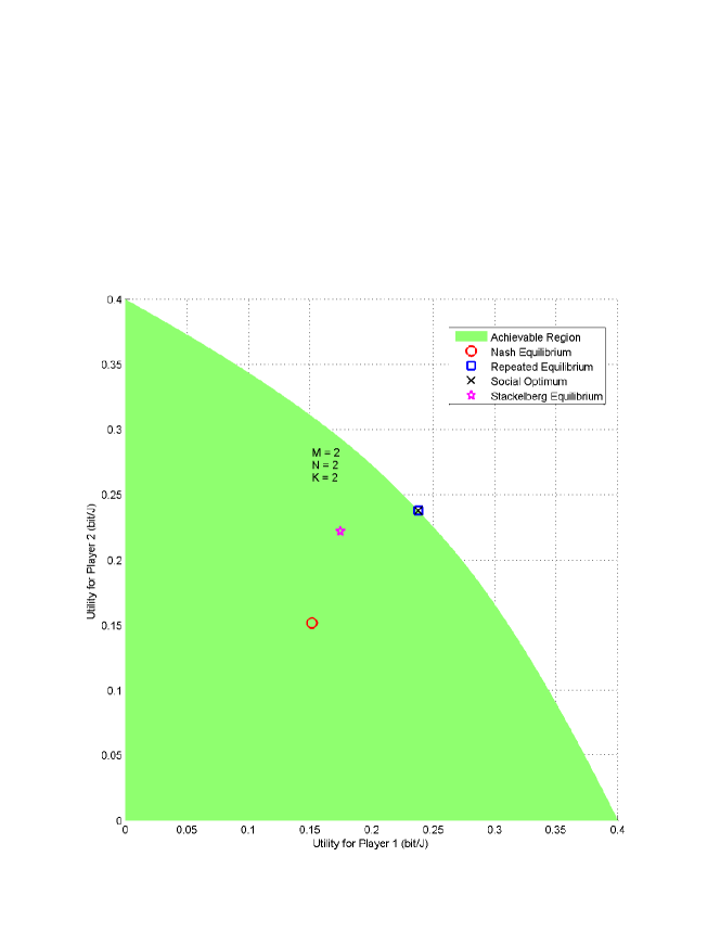
Figure 1: Normalized achievable utility region for $(K,M,N)=(2,2,2)$ plus four important points.

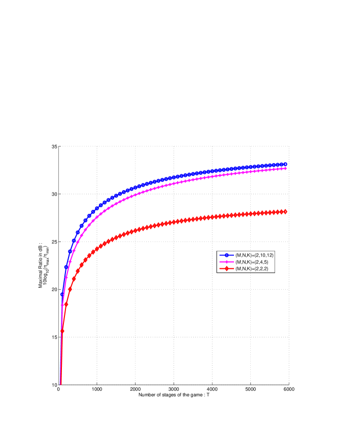
Figure 2: Admissible channel gain dynamics vs. number of stages of the game for $M=2$ and $(K,N)\in\{(2,2),(4,5),(10,12)\}$.

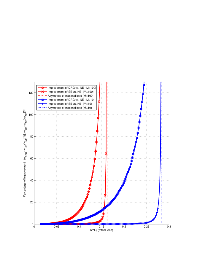
Figure 4: Percentage of improvement of social utility for repeated equilibrium ($w_{DRG}$) and for Stackelberg ($w_{SE}$) vs. Nash equilibrium ($w_{NE}$) in function of the system load ($K/N$).

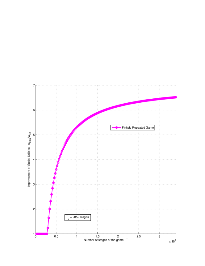
Figure 5: Improvement of social utility for the finitely repeated equilibrium ($w_{FRG}$) vs. Nash equilibrium ($w_{NE}$) in function of the number of stages $T$ of the game.

In this section we consider the same type of scenarios as [3][5] namely random CDMA systems with a spreading factor equal to $N$, the efficiency function $f(x)=(1-e^{-x})^{M}$ and Rayleigh fading channels.
$\star$ The first scenario considered is simple but has the advantage that it can be represented clearly. Consider the scenario $(K,M,N)=(2,2,2)$. Fig. 1 represents the normalized achievable utility region of the one-shot PC game (normalizing the utilities allows one to conduct fair comparisons). Four important points are highlighted: the NE of the one-shot game (circle), the SE (star), the proposed operating/cooperation point studied in Sec. IV-A (square marker), and the point where the social welfare (sum of utilities) is maximized (cross). From this figure it can be seen that: the utility region is convex; a significant gain can be obtained by using a model of repeated games instead of the one-shot model; and the cooperation and optimum social points coincide.
$\star$ Considering the same scenario, the link between the number of stages of the FRG (resp. the stopping probability of the DRG) and channel gain dynamics has been considered. Fig. 2 (resp. 3) represents the quantity $10\log_{10}\left(\frac{\eta^{\mathrm{max}}}{\eta^{\mathrm{min}}}\right)$ as a function of $T$ (resp. of $\lambda$) for $M=2$ and different numbers of transmitters and spreading factors : $(K,N)\in\{(2,2),(4,5),(10,12)\}$. Considering the corresponding figures, the models of RG seem to be suitable not only in scenarios where $|g_{i}|$ models the path loss effects but also the fading effects. Of course if the number of stages is too small or the probability too high, more appropriate models have to be designed.
$\star$ As a third type of numerical results, the performance gain brought by the DRG formulation of the distributed PC problem is assessed. Denote by $w_{NE}$ (resp. $w_{SE}$ and $w_{DRG}$) the efficiency of the NE (resp. SE and RG equilibrium) in terms of social welfare i.e., the sum of utilities of the players. Fig. 4 represents the quantity $\frac{w_{DRG}-w_{NE}}{w_{NE}}$ and $\frac{w_{SE}-w_{NE}}{w_{NE}}$ in percentage as a function of the spectral efficiency $\alpha=\frac{K}{N}$ with $N=128$ and $2\leq K<\frac{N}{\beta^{*}}+1$. The asymptotes $\alpha_{max}=\frac{1}{\beta^{*}}+\frac{1}{N}$ are indicated in dotted lines for different values $M\in\{10,100\}$. The improvement become very significant when the system load is close to $\frac{1}{N}+\frac{1}{\beta^{*}}$, this is because the power at the one-shot game NE becomes large when the system becomes more and more loaded. As explained in [5] for the Stackelberg approach, these gains are in fact limited by the maximum transmit power.
$\star$ At last, Fig. 5 represents the ratio $\frac{{w}_{FRG}}{w_{NE}}$ as a function of the number of stages played (averaged over channel gains). Considering the following constants $(K,M,N)=(35,10,128)$, $P^{max}=10^{-2}$ Watt, $\sigma^{2}=10^{-5}$ Watt, $10\log_{10}(\frac{\eta_{max}}{\eta_{min}})=20$ and the equation (10), a cooperation plan can be settled as soon as $T_{0}=2852$ stages. This curve gives an idea of what a transmitter can gain by cooperating, the normalized gain in terms of utility goes from $1$ to $6$ depending on the number of stages of the game (between $2852$ and $15000$ stages). For example, in a cellular system where power levels are updated with a typical frequency of $1500$ Hz, this would mean that cooperating is a good option if several transmitters are using the same resources for more than $1$ s. The ratio $\frac{{w}_{FRG}}{w_{NE}}$ has a limit when $T\rightarrow+\infty$. The latter is easy to obtain since

$$\frac{{w}_{FRG}}{w_{NE}}=\frac{\phi(\tilde{\gamma})\displaystyle{\sum_{i=1}^{K}R_{i}}\displaystyle{\sum_{t=1}^{T-T_{0}}}|g_{i}(t)|^{2}+\phi(\beta^{*})\displaystyle{\sum_{i=1}^{K}R_{i}}\displaystyle{\sum_{t=T-T_{0}+1}^{T}|g_{i}(t)|^{2}}}{\phi(\beta^{*})\displaystyle{\sum_{i=1}^{K}R_{i}}\displaystyle{\sum_{t=1}^{T}|g_{i}(t)|^{2}}}$$ (14)

where $\phi(x)=\frac{f(x)}{x}\left[1-(K-1)x\right]$. It follows that, for a given $T_{0}$, $\displaystyle{\lim_{T\rightarrow+\infty}}\frac{{w}_{FRG}}{w_{NE}}=\frac{\phi(\tilde{\gamma})}{\phi(\beta^{*})}$.

VI Conclusion

One of the messages of this paper is that taking into account the fact that transmitters interact several times, it is possible to incite selfish transmitters to operate at lower powers, which leads to an equilibrium point that Pareto-dominates the one-shot NE point of [2] and the SE point of [5]. It has been proven that the proposed equilibrium strategies only require individual CSI and a public signal, which is available in many wireless systems. Additionally, this equilibrium is also fair in terms of SINR similarly to the one-shot game NE. In terms of modeling, two models of RG have been analyzed: the finitely RG which is suited to situations where the number of game stages is known, whereas the discounted RG is more suited to situations where it is uncertain or when typical features of wireless networks (delay sensitivity of the network, the fact that users can enter/leave the system, or the fact that transmitters can value the current and future utilities differently) have to be accounted for. An apparent drawback of these two models is the existence of an admissible range for the channel gain dynamics. When only path loss is considered, the corresponding effect is generally negligible. If fading is also considered, simulations have shown that the corresponding impact seems to be limited if the game stopping probability (resp. number of game stages) is reasonably low (resp. high). Otherwise, the proposed model probably needs some refinements such as those proposed in [28] where the author studies the influence of the value of the discount factor on the set of possible equilibrium utilities for the prisoners’ dilemma. As a more general extension of this paper it would be important to apply the proposed approach to other network types such as the interference channel and studying other equilibrium points (depending on the fairness criterion under consideration). At last but not least, the proposed communication and game models, even through there are commonly used, should be refined to propose cooperation plans more robust to imperfect modeling and inherent uncertainty on the quantities used.

Appendix A Proof of Proposition 5

Assume that $\mathcal{U}_{\mathcal{G}}$ is convex. Let $\underline{u}$ be a point of $\mathcal{U}_{\mathcal{G}}$. Define the hyperplane $\mathcal{H}(\underline{u})$, orthogonal to the vector $\left(\frac{1}{|g_{1}|^{2}},...,\frac{1}{|g_{K}|^{2}}\right)$ and containing $\underline{u}$ by: $\mathcal{H}(\underline{u})=\left\{(u_{1}^{\prime},...,u_{K}^{\prime})\in\mathbb{R}_{+}^{K}:\sum_{i=1}^{K}\frac{u_{i}^{\prime}-u_{i}}{|g_{i}|^{2}}=0\right\}$. The key observation to be made is that the point $\underline{\tilde{u}}=(u_{1}(\tilde{p}),...,u_{K}(\tilde{p}))$ given by (9) maximizes the weighted sum $\sum_{i=1}^{K}w_{i}u_{i}$ if $w_{i}=\frac{1}{|g_{i}|^{2}}$. Note that $\underline{\tilde{u}}$ is unique since the solution of $x\left[1-(K-1)x\right]f^{\prime}(x)-f(x)=0$ is unique $\tilde{\underline{p}}=\arg\max_{\underline{p}}\sum_{i=1}^{K}\frac{u_{i}(\underline{p})}{|g_{i}|^{2}}$. By definition, $\underline{\tilde{u}}$ maximizes the Euclidian distance $d(\underline{{u}},\underline{0})$ for all points on the line originating from $\underline{0}$ and directed by the vector $\left(\frac{1}{|g_{1}|^{2}},...,\frac{1}{|g_{K}|^{2}}\right)$, orthogonal to the hyperplane $\mathcal{H}(\underline{\tilde{u}})$. In conclusion, $\underline{\tilde{u}}$ maximizes the sum $\sum_{i=1}^{N}\frac{u_{i}}{|g_{i}|^{2}}$, and because of the convexity of the utility region, no other achievable point can dominate the hyperplane $\mathcal{H}(\underline{\tilde{u}})$, which shows that $\underline{\tilde{u}}$ is PO.
Now assume that $\mathcal{U}_{\mathcal{G}}^{C}$ is convex. Denote by $u_{i}^{\mathrm{max}}$ the maximal utility for player $i$. Define a set of $K$ points $(\hat{u}_{i})_{i\in K}$, such that: $\hat{u}_{i}=(0,\ldots,u_{i}^{\mathrm{max}}+1,\ldots,0)$. Let $\mathcal{P}$ be a polyhedron defined as the subset of $\mathbb{R}^{K}_{+}$ that dominates every hyperplane passing through the OP $\tilde{\underline{u}}$ and a combination of $K-1$ points $\hat{u}_{i}$. As $\mathcal{U}_{\mathcal{G}}^{C}$ is convex, this polyhedron intersects the achievable utility region in a unique point which is the OP $\tilde{\underline{u}}$. Since the positive orthan at the OP is strictly included in the polyhedron, the OP is therefore PO.

Appendix B Proof of Proposition 6

Statement (i). From Sec. II-C we have that

$$\frac{\tilde{u_{i}}}{u_{i}^{L}} =\frac{\frac{f(\tilde{\gamma})}{\tilde{\gamma}}[1-(K-1)\tilde{\gamma}](1+\beta^{*})}{\frac{f(\gamma^{*})}{\gamma^{*}}[1-(K-1)\gamma^{*}\beta^{*}-(K-2)\beta^{*}]}$$ (15)

$$\geq\frac{\frac{f(\tilde{\gamma})}{\tilde{\gamma}}[\beta^{*}-(K-1)\gamma^{*}\beta^{*}+1-(K-1)\gamma^{*}]}{\frac{f(\gamma^{*})}{\gamma^{*}}(\beta^{*}-(K-1)\gamma^{*}\beta^{*}+1-(K-1)\beta^{*})}.$$ (16)

Since by definition $\beta^{*}\geq\gamma^{*}$ we readily see that $\frac{\tilde{u_{i}}}{u_{i}^{L}}\geq 1$.
Statement (ii). From Sec. II-C we have that

$$\frac{\tilde{u_{i}}}{u_{i}^{F}}=\frac{\frac{f(\tilde{\gamma})}{\tilde{\gamma}}[1-(K-1)\tilde{\gamma}](1+\gamma^{*})}{\frac{f(\beta^{*})}{\beta^{*}}[1-(K-1)\gamma^{*}\beta^{*}-(K-2)\beta^{*}]}$$ (17)

$$\geq\frac{\frac{f(\tilde{\gamma})}{\tilde{\gamma}}\left\{1-\tilde{\gamma}[(K-1)\gamma^{*}+K-2]\right\}}{\frac{f(\beta^{*})}{\beta^{*}}\left\{1-\beta^{*}[(K-1)\gamma^{*}+K-2]\right\}}.$$ (18)

We want to prove that this ratio is greater than or equal to $1$. We consider the quantity :

$$\varphi_{[\tilde{\gamma}_{K},\beta^{*}]}(K) =\frac{f(\tilde{\gamma}_{K})}{\tilde{\gamma}_{K}}\left\{1-\tilde{\gamma}_{K}[(K-1)\gamma^{*}_{K}+K-2]\right\}$$

$$-\frac{f(\beta^{*})}{\beta^{*}}\left\{1-\beta^{*}[(K-1)\gamma^{*}_{K}+K-2]\right\}$$

$$=K(f(\beta^{*})-f(\tilde{\gamma}_{K}))(\gamma_{K}^{*}+1)+\frac{f(\tilde{\gamma}_{K})}{\tilde{\gamma}_{K}}$$

$$-\frac{f(\beta^{*})}{\beta^{*}}-(f(\beta^{*})-f(\tilde{\gamma}_{K}))(\gamma^{*}_{K}+2)$$

$$\geq K(f(\beta^{*})-f(\tilde{\gamma}_{K}))(\tilde{\gamma}_{K}+1)+\frac{f(\tilde{\gamma}_{K})}{\tilde{\gamma}_{K}}$$ (21)

$$-\frac{f(\beta^{*})}{\beta^{*}}-(f(\beta^{*})-f(\tilde{\gamma}_{K}))(\beta^{*}+2)$$ (22)

As $\tilde{\gamma}_{K}$ goes to zero as $K$ goes to infinity, ($\tilde{\gamma}_{K}\leq\frac{1}{K-1}$) and by hypothesis $f(0)=0$, $\lim_{x\rightarrow 0}\frac{f(x)}{x}=0$ :

$$\lim_{K\rightarrow+\infty}\varphi_{[\tilde{\gamma}_{K},\beta^{*}]}(K)$$ (23)

$$\geq\lim_{K\rightarrow+\infty}K[(f(\beta^{*})-f(\tilde{\gamma}_{K}))(\tilde{\gamma}_{K}+1)]$$ (24)

$$+\frac{f(\tilde{\gamma}_{K})}{\tilde{\gamma}_{K}}-\frac{f(\beta^{*})}{\beta^{*}}-(f(\beta^{*})-f(\tilde{\gamma}_{K}))(\beta^{*}+2)$$

$$\geq\lim_{K\rightarrow+\infty}K(f(\beta^{*}))-\frac{f(\beta^{*})}{\beta^{*}}-(f(\beta^{*}))(\beta^{*}+2)=+\infty$$ (25)

In conclusion, the sequence $(\varphi_{[\tilde{\gamma}_{K},\beta^{*}]}(K))_{K\geq 2}$ is strictly increasing and its limit is $+\infty$. There exists an integer $K_{0}$ such that for all $K\geq K_{0}$, $\varphi_{[\tilde{\gamma}_{K},\beta^{*}]}(K)>0$. This implies that $u_{i}(\tilde{\underline{p}})>u_{i}^{F}$.

Appendix C Proof of Proposition 7

The goal is to show that $\forall i\in K,\frac{u_{i}(\tilde{\underline{p}})}{u_{i}(\underline{p}^{*})}=\frac{\frac{f(\tilde{\gamma})}{\tilde{\gamma}}[1-(K-1)\tilde{\gamma}]}{\frac{f(\gamma^{*})}{\gamma^{*}}[1-(K-1)\gamma^{*}]}$ is greater than or equal to one. For this, consider the function $\phi(x)=\frac{f(x)}{x}\left[1-(K-1)x\right]$. The derivative of $\phi$ is $\phi^{\prime}(x)=\frac{x(1-(K-1)x)f^{\prime}(x)-f(x)}{x^{2}}$ which vanishes in unique point namely, in $\tilde{\gamma}$. Therefore the function $\phi$ is strictly increasing on $]0,\tilde{\gamma}[$ and strictly decreasing on $]\tilde{\gamma},+\infty[$ and thus reaches its maximum in $\tilde{\gamma}$, which concludes the proof.

Appendix D Proof of Theorems 8 and 9

The proofs are provided in the general case where the PC game is repeated for different channel realizations (DSPC). At a game stage $t$ a transmitter has therefore to consider future realizations of the channels, which are unknown at stage $t$. To tackle this issue we use a dynamic programming principle [21], which is standard in repeated game. Let us define $\bar{u_{i}}=\max_{\underline{p}}u_{i}(\underline{p})=\frac{R_{i}|g_{i}|^{2}f(\beta^{*})}{\sigma^{2}\beta^{*}}$, the maximal utility player $i$ can get for a fixed channel gain $|g_{i}|^{2}$. First consider the FRG. It is clear that during the last $T_{0}$ stage, the players play the one-shot NE. Thus no deviation over this period can be profitable to any player. We now consider that a player deviates during the first $T-T_{0}$ stages. His deviation utility is bounded by $\bar{u}_{i}$ and he will be punished at his minmax level in the next stage. Suppose the deviator deviates at stage $t\leq T-T_{0}$. Denote by $\stackrel{{\scriptstyle\frown}}{{u_{i}}}=\min_{\underline{p}_{-i}}\max_{p_{i}}u_{i}(\underline{p})$ with $\underline{p}_{-i}=(p_{1},...,p_{i-1},p_{i+1},...,p_{K})$. The deviation utility of the FRG is upper-bounded as:

$$\sum_{s=1}^{t-1}\tilde{u_{i}}(\underline{p}(s))+\bar{u_{i}}(\underline{p}(t))+\sum_{s=t+1}^{T}\mathbb{E}_{\mathbf{g}}[\stackrel{{\scriptstyle\frown}}{{u}}_{i}(\underline{p}(s))]$$

$$\leq\sum_{s=1}^{T-T_{0}-1}\tilde{u_{i}}(\underline{p}(s))+\bar{u_{i}}(\underline{p}(T-T_{0}))+\sum_{s=T-T_{0}+1}^{T}\mathbb{E}_{\mathbf{g}}[\stackrel{{\scriptstyle\frown}}{{u_{i}}}(\underline{p}(s))]$$

The equilibrium condition for the FRG at stage $t$ writes as:

$$\sum_{s=1}^{T-T_{0}-1}\tilde{u_{i}}(\underline{p}(s))+\bar{u_{i}}(\underline{p}(T-T_{0}))+\sum_{s=T-T_{0}+1}^{T}\mathbb{E}_{\mathbf{g}}[\stackrel{{\scriptstyle\frown}}{{u_{i}}}(\underline{p}(s))]$$

$$\leq\sum_{s=1}^{T-T_{0}-1}\tilde{u_{i}}(\underline{p}(s))+\tilde{u_{i}}(\underline{p}(T-T_{0}))+\sum_{s=T-T_{0}+1}^{T}\mathbb{E}_{\mathbf{g}}[u_{i}^{*}(\underline{p}(s))]$$

$$\Longleftrightarrow\quad\bar{u_{i}}(\underline{p}(t))+\sum_{s=T-T_{0}+1}^{T}\mathbb{E}_{\mathbf{g}}[\stackrel{{\scriptstyle\frown}}{{u_{i}}}(\underline{p}(s))]$$

$$\leq\tilde{u_{i}}(\underline{p}(t))+\sum_{s=T-T_{0}+1}^{T}\mathbb{E}_{\mathbf{g}}[u_{i}^{*}(\underline{p}(s))]$$

$$\Longleftrightarrow\quad|g_{i}|^{2}\frac{f(\beta^{*})}{\beta^{*}}+\sum_{s=T-T_{0}+1}^{T}\mathbb{E}_{\mathbf{g}}[\frac{|g_{i}|^{2}f(\beta^{*})}{\beta^{*}\left(\sum_{j\in\mathcal{K}\backslash i}p_{j}^{\max}|g_{j}|^{2}+\sigma^{2}\right)}]$$

$$\leq|g_{i}|^{2}\frac{f(\tilde{\gamma})(1-(K-1)\tilde{\gamma})}{\tilde{\gamma}}+\sum_{s=T-T_{0}+1}^{T}\mathbb{E}_{\mathbf{g}}[|g_{i}|^{2}]\frac{f(\beta^{*})(1-(K-1)\beta^{*})}{\beta^{*}}.$$

Now we want to show that the last inequality is verified under the sufficient condition of Theorem $8$. The sufficient condition of Theorem $8$ implies that:

$$\eta_{i}^{\mathrm{max}}\frac{f(\beta^{*})}{\beta^{*}}-\eta_{i}^{\mathrm{min}}\frac{f(\tilde{\gamma})(1-(K-1)\tilde{\gamma})}{\tilde{\gamma}}$$

$$\leq T_{0}\left[\;\eta_{i}^{\mathrm{min}}\frac{f(\beta^{*})(1-(K-1)\beta^{*})}{\beta^{*}}-\frac{\eta_{i}^{\mathrm{max}}f(\beta^{*})}{\beta^{*}\left(\sum_{j\in\mathcal{K}\backslash i}p_{j}^{\max}\eta_{i}^{\mathrm{min}}+\sigma^{2}\right)}\right]$$

$$\Longrightarrow\eta_{i}^{\mathrm{max}}\frac{f(\beta^{*})}{\beta^{*}}+T_{0}\frac{\eta_{i}^{\mathrm{max}}f(\beta^{*})}{\beta^{*}\left(\sum_{j\in\mathcal{K}\backslash i}p_{j}^{\max}\eta_{i}^{\mathrm{min}}+\sigma^{2}\right)}$$

$$\leq\eta_{i}^{\mathrm{min}}\frac{f(\tilde{\gamma})(1-(K-1)\tilde{\gamma})}{\tilde{\gamma}}+T_{0}\eta_{i}^{\mathrm{min}}\frac{f(\beta^{*})(1-(K-1)\beta^{*})}{\beta^{*}}$$

$$\Longrightarrow\eta_{i}^{\mathrm{max}}\frac{f(\beta^{*})}{\beta^{*}}+\sum_{s=T-T_{0}+1}^{T}\frac{\eta_{i}^{\mathrm{max}}f(\beta^{*})}{\beta^{*}\left(\sum_{j\in\mathcal{K}\backslash i}p_{j}^{\max}\eta_{i}^{\mathrm{min}}+\sigma^{2}\right)}$$

$$\leq\eta_{i}^{\mathrm{min}}\frac{f(\tilde{\gamma})(1-(K-1)\tilde{\gamma})}{\tilde{\gamma}}+\sum_{s=T-T_{0}+1}^{T}\eta_{i}^{\mathrm{min}}\frac{f(\beta^{*})(1-(K-1)\beta^{*})}{\beta^{*}},$$

The worst case scenario for stochastic channel gains implies the average case scenario. The condition of theorem 8 is sufficient for the desired equilibrium condition hold at each stage $t$ of the FRG. This concludes the proof for the FRG. Consider now the equilibrium condition for the DRG at stage $t$ :

$$\lambda\bar{u_{i}}(\underline{p}^{t})+\sum_{s\geq t+1}\lambda(1-\lambda)^{s-t}\mathbb{E}_{\mathbf{g}}[u_{i}^{*}(\underline{p}^{s})]$$

$$\leq\lambda\tilde{u_{i}}(\underline{p}^{t})+\sum_{s\geq t+1}\lambda(1-\lambda)^{s-t}\mathbb{E}_{\mathbf{g}}[\tilde{u_{i}}(\underline{p}^{s})]$$

$$\Longleftrightarrow \lambda|g_{i}|^{2}\frac{f(\beta^{*})}{\beta^{*}}$$

$$+ \sum_{s\geq t+1}\lambda(1-\lambda)^{s-t}\mathbb{E}_{\mathbf{g}}[|g_{i}|^{2}]\frac{f(\beta^{*})(1-(K-1)\beta^{*})}{\beta^{*}}$$

$$\leq \lambda|g_{i}|^{2}\frac{f(\tilde{\gamma})(1-(K-1)\tilde{\gamma})}{\tilde{\gamma}}$$

$$+ \sum_{s\geq t+1}\lambda(1-\lambda)^{s-t}\mathbb{E}_{\mathbf{g}}[|g_{i}|^{2}]\frac{f(\tilde{\gamma})(1-(K-1)\tilde{\gamma})}{\tilde{\gamma}}$$

$$\Longleftrightarrow \lambda|g_{i}|^{2}\left[\frac{f(\beta^{*})}{\beta^{*}}-\frac{f(\tilde{\gamma})(1-(K-1)\tilde{\gamma})}{\tilde{\gamma}}\right]$$

$$\leq \sum_{s\geq t+1}\lambda(1-\lambda)^{s-t}\mathbb{E}_{\mathbf{g}}\left[|g_{i}|^{2}\right]$$

$$\times \left[\frac{f(\tilde{\gamma})(1-(K-1)\tilde{\gamma})}{\tilde{\gamma}}-\frac{f(\beta^{*})(1-(K-1)\beta^{*})}{\beta^{*}}\right]$$

The equilibrium condition for the DRG can be obtained by following the same reasoning as for the FRG.

Mael Le Treust earned his Diplôme d’Étude Approfondies (M.Sc.) degree in Optimization, Game Theory & Economics (OJME) from the Université de Paris VI (UPMC), France in 2008. He is currently pursuing his Ph.D. degree at the Laboratoire des signaux et systèmes (joint laboratory of CNRS, Supélec, Université de Paris XI), Gif-sur-Yvette, France. He was also a Math TA at the Université de Paris I (Panthéon-Sorbonne) and Université de Paris VI (UPMC), France. His research interests include game theory, wireless communications and information theory.

Samson Lasaulce received his BSc and Agrégation degree in Applied Physics from École Normale Supérieure (Cachan) and his MSc and PhD in Signal Processing from École Nationale Supérieure des Télécommunications de Paris (ENST). He has been working with Motorola Labs (1999, 2000, 2001) and France Télécom R+D (2002, 2003). Since 2004, he has joined the CNRS and Supélec and is Chargé d’Enseignement at École Polytechnique. His broad interests lie in the areas of communications, signal processing, information theory and game theory for wireless communications.

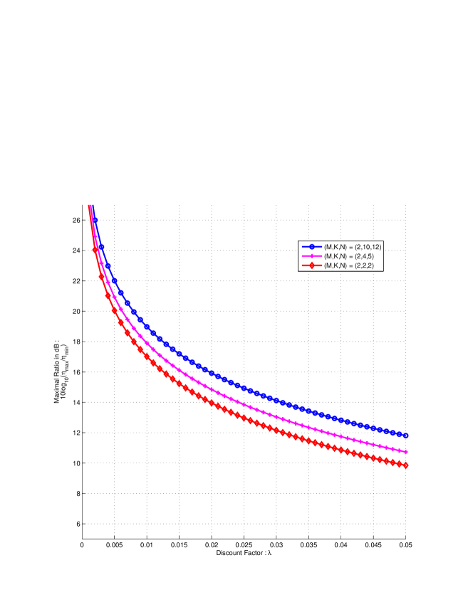
Figure 3: Admissible channel gain dynamics vs. discount factor for $M=2$ and $(K,N)\in\{(2,2),(4,5),(10,12)\}$.

References

- [1] V. Shah, N. B. Mandayam, and D. J. Goodman, “Power Control for Wireless Data based on Utility and Pricing”, in IEEE Proc. of the 9th Intl. Symp. on Indoor and Mobile Radio Commun. (PIMRC), Boston, USA, Vol. 3, pp. :1427–1432, Sep 1998.
- [2] D. J. Goodman and N. B. Mandayam, “Power control for wireless data”, IEEE Person. Comm., Vol. 7, No. 2, pp. 48–54, 2000.
- [3] F. Meshkati, M. Chiang, H. V. Poor and S. C. Schwartz, “A game-theoretic approach to energy-efficient power control in multi-carrier CDMA systems”, IEEE Journal on Selected Areas in Communications, Vol. 24, No. 6, pp. 1115–1129, June 2006.
- [4] C. U. Saraydar, N. B. Mandayam and D. J. Goodman, “Efficient power control via pricing in wireless data networks”, IEEE Trans. on Communications, Vol. 50, No. 2, pp. 291–303, Feb. 2002.
- [5] S. Lasaulce, Y. Hayel, R. El Azouzi and M. Debbah, “Introducing hierarchy in energy games”, IEEE Trans. on Wireless Comm., Vol. 8, No. 7, pp. 3833–3843, Jul. 2009.
- [6] V. H. Stackelberg, “Marketform und Gleichgewicht”, Oxford University Press, 1934.
- [7] R. J. Aumann, “Survey of repeated games”, Essays in game theory and mathematical economics in honor of Oskar Morgenstern, edited by R. J. Aumann, Wissenschaftsverlag, Bibliographisches Institut, Mannheim, Wien, Zurich, pp. 11-42, 1981.
- [8] S. Sorin, “Repeated Games with Complete Information”, In: R. Aumann, S. Hart (eds.), Handbook of game theory with economic applications, Vol. 1, pp. 71-107, 1992.
- [9] J. F. Mertens, S. Sorin, and S. Zamir, “Repeated Games, Parts A,B,C”, CORE Discussion Papers, 1994.
- [10] Benoit, J. P. and V. Krishna, “Finitely Repeated Games” Econometrica, Vol. 39, No. 10, pp. 905–922, 1985.
- [11] D Fudenberg, E Maskin, “The folk theorem in repeated games with discounting or with incomplete information”, Econometrica: Journal of the Econometric Society, Vol. 54, No. 3, pp. 533–554, 1986.
- [12] R. Etkin, A. Parekh and D. Tse, “Spectrum Sharing for Unlicensed Bands”, IEEE Journal on Selected Areas on Communications, Special issue on adaptive, Spectrum Agile and Cognitive Wireless Networks, Vol. 25, No. 3, pp. 517-528, April 2007.
- [13] L. Lai and H. El Gamal, “The Water-Filling Game in Fading Multiple-Access Channels”, IEEE Trans. on Information Theory, Vol. 54, No. 5, pp. 2110–2122, May 2008.
- [14] Y. Wu, B. Wang, K. J. R. Liu, and T. C. Clancy, “Repeated Open Spectrum Sharing Game with Cheat-Proof Strategies”, IEEE Trans. on Wireless Comm., Vol. 8, No. 4, pp. 1922–1933, Apr. 2009.
- [15] A. D. Wyner, “Recent results in Shannon theory”, IEEE Trans. on Inform. Theory, Vol. 20, Issue 1, pp. 2–10, Jan. 1974.
- [16] T. Cover, “Some advances in broadcast channels”, in Advances in Comm. Systems, Vol. 4, Academic Press, 1975.
- [17] E. V. Belmega, S. Lasaulce and M. Debbah, “Power allocation games for MIMO multiple access channels with coordination”, IEEE Trans. on Wireless Communications, Vol. 8, No. 5, May 2009.
- [18] V. Rodriguez, “An Analytical Foundation for Resource Management in Wireless Communication”, IEEE Proc. of Globecom, 2003.
- [19] F. Meshkati, H. V. Poor, S. C. Schwartz, and N. B. Mandayam, “An Energy-Efficient Approach to Power Control and Receiver Design in Wireless Data Networks”, IEEE Trans. on Comm., Vol. 53, No. 11, Nov. 2005.
- [20] E. V. Belmega and S. Lasaulce, “An information-theoretic look at MIMO energy-efficient communications”, ACM Proc. of the Intl. Conf. on Performance Evaluation Methodologies and Tools (VALUETOOLS), Pisa, Italy, Oct. 2009.
- [21] L. Shapley, “Stochastic Games”, Proc. of Nat. Aca. of Science, Vol. 39, pp. 1095 -1100, 1953.
- [22] Fudenberg, D. and Levine, D. and Maskin, E., “The Folk Theorem with Imperfect Public Information”, Econometrica, Vol. 62, No. 5, pp. 997-1039, Sep. 1994.
- [23] T. Tomala, “Pure equilibria of repeated games with public observation”, International Journal of Game Theory (IJGT), Vol. 27, No. 1, pp. 93–109, 1998.
- [24] D. Goodman and N. Mandayam, “Network assisted power control for wireless data”, Mobile Networks and Applications, Vol. 6, No. 5, pp. 409–415, 2001.
- [25] Robert J. Aumann, “The Core of a Cooperative Game Without Side Payments” Trans. of the A.M.S., Vol. 98, No 3, pp. 539–552, 1961.
- [26] J. F. Mertens, “A note on the characteristic function of supergames” Intl. Journal of Game Theory, Vol. 9, No. 4, pp. 189–190, 1980.
- [27] R. Selten, “Spieltheoretische behandlung eines oligopolmodells mit nachfragetragheit”, Zeits. fuer die gesamte Staatswissenschaft, 1965.
- [28] S. Sorin, “On Repeated Games with Complete Information”, Mathematics of Operations Research, Vol. 11, No. 1, pp. 147–160, 1986.