Simulation of Z(3) walls and string production via bubble nucleation in a quark-hadron transition

Abstract

We study the dynamics of confinement-deconfinement (C-D) phase transition in the context of relativistic heavy-ion collisions within the framework of effective models for the Polyakov loop order parameter. We study the formation of $Z(3)$ walls and associated strings in the initial transition from the confining (hadronic) phase to the deconfining (QGP) phase via the so called Kibble mechanism. Essential physics of the Kibble mechanism is contained in a sort of domain structure arising after any phase transition which represents random variation of the order parameter at distances beyond the typical correlation length. We implement this domain structure by using the Polyakov loop effective model with a first order phase transition and confine ourselves with temperature/time ranges so that the first order C-D transition proceeds via bubble nucleation, leading to a well defined domain structure. The formation of $Z(3)$ walls and associated strings results from the coalescence of QGP bubbles expanding in the confining background. We investigate the evolution of the $Z(3)$ wall and string network. We also calculate the energy density fluctuations associated with $Z(3)$ wall network and strings which decay away after the temperature drops below the quark-hadron transition temperature during the expansion of QGP. We discuss evolution of these quantities with changing temperature via Bjorken’s hydrodynamical model and discuss possible experimental signatures resulting from the presence of $Z(3)$ wall network and associate strings.

Key words: quark-hadron transition, relativistic heavy-ion collisions, Z(3) domain walls

I INTRODUCTION

Search for the quark-gluon plasma (QGP) at relativistic heavy-ion collision experiments (RHICE) has reached a very exciting stage with the ongoing experiments at RHIC and with the upcoming heavy-ion experiments at the Large Hadron Collider. No one doubts that the QGP phase has already been created at RHIC but conclusive evidence for the same is still lacking. Many signatures have been proposed for the detection of the QGP phase heinz and these have been thoroughly investigated both theoretically and experimentally. Along with continued investigation of these important signatures of QGP, there is a need for investigating novel signals exploring qualitatively non-trivial features of the QGP phase and/or the quark-hadron phase transition.

With this view we focus on the non-trivial vacuum structure of the QGP phase which arises when one uses the expectation value of the Polyakov loop $l(x)$ as the order parameter for the confinement-deconfinement phase transition lary . This order parameter transforms non-trivially under the center $Z(3)$ of the color SU(3) group and is non-zero above the critical temperature $T_{c}$. This breaks the global $Z(3)$ symmetry spontaneously above $T_{c}$, while the symmetry is restored below $T_{c}$ in the confining phase where this order parameter vanishes. In the QGP phase, due to spontaneous breaking of the discrete $Z(3)$ symmetry, one gets domain walls (interfaces) which interpolate between different $Z(3)$ vacua. The properties and physical consequences of these $Z(3)$ interfaces have been discussed in the literaturezn . It has been suggested that these interfaces should not be taken as physical objects in the Minkowski space smlg . Similarly, it has also been subject of discussion whether it makes sense to talk about this $Z(3)$ symmetry in the presence of quarks qurk1 . However, we will follow the approach where the presence of quarks is interpreted as leading to explicit breaking of $Z(3)$ symmetry, lifting the degeneracy of different $Z(3)$ vacua qurk2 ; psrsk ; psrsk2 ; z3lnr . Thus, with quarks, even planar $Z(3)$ interfaces do not remain static and move away from the region with the unique true vacuum. Our main discussion will be for the pure gauge theory which we discuss first. Later we will briefly comment on the situation with quarks. A detailed study with inclusion of quark effects is postponed for a future work.

In earlier works some of us had shown that there are novel topological string defects which form at the intersection of the three $Z(3)$ interfaces. These strings are embedded in the QGP phase and their cores consist of the confining phase. Structure of these strings and interfaces were discussed in these earlier works z3str . It was also shown that reflection of quarks from collapsing $Z(3)$ interfaces can lead to large scale baryon inhomogeneities in the early universe znb . This effect is also utilized to argue for $P_{T}$ enhancement of quarks of heavy flavor (consecutively corresponding hadrons) in relativistic heavy-ion collisions apm .

In this paper we carry out numerical simulation of formation of these $Z(3)$ interfaces and associated strings at the initial confinement-deconfinement transition which is believed to occur during the pre-equilibrium stage in relativistic heavy-ion collision experiments. For the purpose of numerical simulation we will model this stage as a quasi-equilibrium stage with an effective temperature which first rises (with rapid particle production) to a maximum temperature $T_{0}>T_{c}$, where $T_{c}$ is the critical temperature for the confinement-deconfinement phase transition, and then decreases due to continued plasma expansion.

We use the effective potential for the Polyakov loop expectation value $l(x)$ as proposed by Pisarski psrsk ; psrsk2 to study the confinement-deconfinement (C-D) phase transition. Within this model, the C-D transition is weakly first order. Even though Lattice results show that quark-hadron transition is most likely a smooth cross-over at zero chemical potential, in the present work we will use this first order transition model to discuss the dynamical details of quark-hadron transition. One reason for this is that our study is in the context of relativistic heavy-ion collision experiments (RHICE) where the baryon chemical potential is not zero. For not too small values of the chemical potential, the quark-hadron phase transition is expected to be of first order, so this may be the case relevant for us any way (especially when collision energy is not too high). Further, our main interest is in determining the structure of the network of Z(3) domain walls and strings resulting during the phase transition. These objects will form irrespective of the nature of the transition, resulting entirely from the finite correlation lengths in a fast evolving system, as shown by Kibble kbl . The Kibble mechanism was first proposed for the formation of topological defects in the context of the early universe kbl , but is now utilized extensively for discussing topological defects production in a wide variety of systems from condensed matter physics to cosmology zrk . Essential ingredient of the Kibble mechanism is the existence of uncorrelated domains of the order parameter which result after every phase transition occurring in finite time due to finite correlation length. A first order transition allows easy implementation of the resulting domain structure especially when the transition proceeds via bubble nucleation. With this view, we use the Polyakov loop model as in psrsk ; psrsk2 to model the phase transition and confine ourselves with temperature/time ranges so that the first order quark-hadron transition proceeds via bubble nucleation.

The $Z(3)$ wall network and associated strings (as mentioned above) formed during this early confinement-deconfinement phase transition evolve in an expanding plasma with decreasing temperature. Eventually when the temperature drops below the deconfinement-confinement phase transition temperature $T_{c}$, these $Z(3)$ walls and associated strings will melt away. However they may leave their signatures in the form of extended regions of energy density fluctuations (as well as $P_{T}$ enhancement of heavy-flavor hadrons apm ). We make estimates of these energy density fluctuations which can be compared with the experimental data. Especially interesting will be to look for extended regions of large energy densities in space-time reconstruction of hadron density (using hydrodynamic models). In our model, we expect energy density fluctuations in event averages (representing high energy density regions of domain walls/strings), as well as event-by-event fluctuations as the number/geometry of domain walls/strings and even the number of QGP bubbles, varies from one event to the other. A detailed analysis of energy fluctuations, especially the event-by-event fluctuations, is postponed for a future work.

We also determine the distribution/shape of $Z(3)$ wall network and its evolution. In particular, our results provide an estimate of domain wall velocities (for the situations studied) to range from 0.5 to 0.8. These results provide crucial ingredients for a detailed study of the effects of collapsing $Z(3)$ walls on the $P_{T}$ enhancement of heavy flavor hadrons znb ; apm in RHICE. We emphasize that the presence of $Z(3)$ walls and string may not only provide a qualitatively new signature for the QGP phase in these experiments, it may provide the first (and may be the only possible) laboratory study of such topological objects in a relativistic quantum field theory system.

The paper is organized in the following manner. In section II, we discuss the Polyakov loop model of confinement-deconfinement phase transition. We describe the effective potential proposed by Pisarski psrsk and discuss the structure of the $Z(3)$ walls and associated strings. In section III, we present the physical picture of the formation of these $Z(3)$ walls and associated strings in the confinement-deconfinement phase transition via the Kibble mechanism which provides a general framework for the production of topological defects in symmetry breaking phase transitions. We confine ourselves with temperature/time ranges so that the first order transition (in the Pisarski model) proceeds via bubble nucleation. The other possibility of spinodal decomposition is of completely different nature and we will present it in a future work. (We mention here that a simulation of spinodal decomposition in Polyakov loop model has been carried out in ref. dumitru , where fluctuations in the Polyakov loop are investigated in detail. In comparison, the main focus of our work is on the topological objects, Z(3) walls, and strings, and energy density fluctuations resulting therefrom.) In section IV, we discuss the calculation of the profile of the critical bubble using bounce technique clmn and also the estimates of nucleation rates for bubbles for the temperature/time range relevant for RHICE. Section V presents the numerical technique of simulating the phase transition via random nucleation of bubbles. In section VI we discuss the issue of the effects of quarks in our model. Section VII presents the results of the numerical simulations. Here we discuss distribution of $Z(3)$ wall/string network formed due to coalescence of QGP bubbles (in a confining background). We also calculate the energy density fluctuations associated with $Z(3)$ wall network and strings. We discuss evolution of these quantities with changing temperature via Bjorken’s hydrodynamical model. In section VIII we discuss possible experimental signatures resulting from the presence of $Z(3)$ wall network and associate strings. Section IX presents conclusions.

II THE POLYAKOV LOOP MODEL

We first discuss the case of pure SU(N) gauge theory. We will later discuss briefly the case with quarks. The order parameter for the confinement-deconfinement (C-D) phase transition is the expectation value of the Polyakov loop $\it l(x)$ which is defined as

$$\it l(x)=(1/N)tr(Pexp(ig\int^{\beta}_{0}A_{0}(x,\tau)d\tau))$$ (1)

Here P denotes the path ordering, g is the gauge coupling, and $\beta=1/T$, where T is the temperature. $A_{0}(x,\tau)\equiv A_{0}^{a}(x,\tau)T_{a}$, $T_{a}$ being the generators of SU(N) in the fundamental representation, is the time component of the vector potential at spatial position $\it{x}$ and Euclidean time $\tau$. Under a global Z(N) symmetry transformation, $\it l(x)$ transforms as

$$\it l(x)\rightarrow{exp(2{\pi}in/N)\it l(x)},\>n=0,1,...(N-1)$$ (2)

The expectation value of $l(x)$ is related to $e^{-\beta F}$ where $F$ is the free energy of an infinitely heavy test quark. For temperatures below $T_{c}$, in the confined phase, the expectation value of Polyakov loop is zero corresponding to the infinite free energy of an isolated test quark. (Hereafter, we will use the same notation $l(x)$ to denote the expectation value of the Polyakov loop.) Hence the Z(N) symmetry is restored below $T_{c}$. Z(N) symmetry is broken spontaneously above $T_{c}$ where $l(x)$ is non-zero corresponding to the finite free energy of the test quark. For QCD, $N=3$, and we take the effective theory for the Polyakov loop as proposed by Pisarski psrsk ; psrsk2 . The effective Lagrangian density is given by

$$L={N\over g^{2}}|{\partial_{\mu}\it l}|^{2}{T^{2}}-V(\it l)$$ (3)

$V(\it l)$ is the effective potential for the Polyakov loop

$$V(\it l)=({-b_{2}\over 2}|\it l|^{2}-{b_{3}\over 6}(\it l^{3}+(\it l^{\ast})^{3})+\frac{1}{4}(|\it l|^{2})^{2}){b_{4}{T^{4}}}$$ (4)

The values of various parameters are fixed to reproduce the lattice results scav ; latt for pressure and energy density of pure SU(3) gauge theory. We make the same choice and give those values below. The coefficients $b_{3}$ and $b_{4}$ have been taken as, $b_{3}=2.0$ and $b_{4}=0.6016$. We will take the same value of $b_{2}$ for real QCD (with three massless quark flavors), while the value of $b_{4}$ will be rescaled by a factor of 47.5/16 to account for the extra degrees of freedom relative to the degrees of freedom of pure SU(3) gauge theory scav . The coefficient $b_{2}$ is temperature dependent scav . $b_{2}$ is taken as, $b_{2}(r)=(1-1.11/r)(1+0.265/r)^{2}(1+0.3/r)^{3}-0.487$, where r is taken as T/$T_{c}$. With the coefficients chosen as above, the expectation value of order parameter approaches to $\it x=b_{3}/2+\frac{1}{2}\sqrt{b_{3}^{2}+4b_{2}(T=\infty)}$ for temperature $T\rightarrow\infty$. As in psrsk2 , we use the normalization such that the expectation value of order parameter $\it l_{0}$ goes to unity for temperature $T\rightarrow\infty$. Hence the fields and the coefficients in $V(l)$ are rescaled as $\it l\rightarrow l/x$, $b_{2}(T)\rightarrow b_{2}(T)/x^{2}$, $b_{3}\rightarrow b_{3}/x$ and $b_{4}\rightarrow b_{4}x^{4}$ to get proper normalization of $\it l_{0}$.

For the parameters chosen as above, the value of $T_{c}$ is taken to be 182 MeV. We see that the $b_{3}$ term in Eq.(4) gives a cos(3$\theta$) term, leading to Z(3) degenerate vacua structure. Here, the shape of the potential is such that there exists a metastable vacuum upto a temperature $\sim$ 250 MeV. Hence first order transition via bubble nucleation is possible only upto $T=250$ MeV. We show the plot of V$(\it l)$ in $\theta=0$ direction in Fig.(1a) for a value of temperature T = 185 MeV. This shows the metastable vacuum at $\it l=0$. Fig.(1b) shows the structure of vacuum by plotting V($\it l$) as a function of $\theta$ for fixed $\it l_{0}$, where $l_{0}$ is the vacuum expectation value of $V(\it l)$ at $T=185$ MeV.

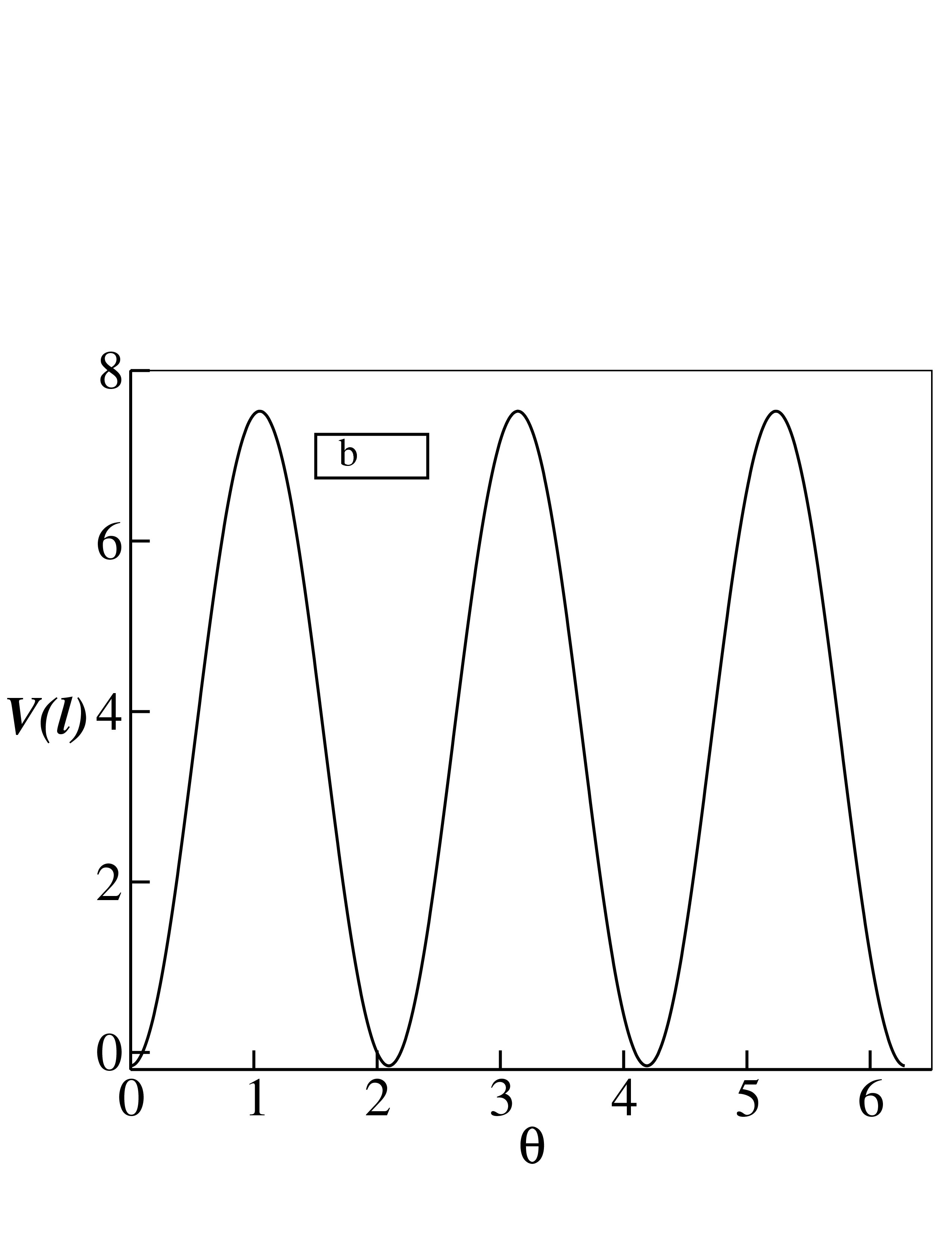
Figure 1:

(a) Plot of $V(l)$ in $\theta=0$ direction for $T=185MeV$ showing the metastable vacuum at $l=0$. In (a) and (b), plots of $V$ are given in units of $T_{c}^{4}$. The value of critical temperature is taken to be $T_{c}\simeq 182MeV$. The $Z(3)$ structure of the vacuum can be seen in (b) in the plot of the potential $V(l)$ as a function of $\theta$ for fixed $|l|=l_{0}$. Here, $l_{0}$ corresponds to the absolute minimum of $V(l)$.

In Fig.(1b), the three degenerate vacua are separated by large barrier in between them. While going from one vacuum to another vacuum, the field configuration is determined from the field equations. For the case of degenerate vacua, there are time independent solutions which have planar symmetry. These solutions are called domain wall. For the non-degenerate case, as will be appropriate for the case when quarks are included as dynamical degrees of freedom in discussing the quark hadron transition, the solutions of the interfaces separating these vacua will be similar to the bounce solutions clmn , though the standard bounce techniques need to be extended for the case of complex scalar field. The resulting planar domain wall solutions will not be static. As mentioned above, we will be neglecting such effects of quarks, and hence will discuss the case of degenerate vacua only. Later, in section VI, we will examine the justification of using the approximation of neglecting quark effects.

In physical space, after the phase transition, regions with different Z(3) vacua are separated by domain walls. Inside a domain wall, $|l|$ becomes very small as $T\rightarrow T_{c}$ z3str . In ref.z3str the intersection of the three Z(3) domain walls was considered and, using topological arguments, it was then shown that at the line-like intersection of these interfaces, the order parameter $l(x)$ should vanish. This leads to a topological string configuration with core of the string being in the confining phase. Properties of these new string configurations were determined in z3str using the model of Eq.(3). This string configuration is interesting, especially when we note that such a string has exactly reverse physical behavior compared to the standard QCD string. The QCD string exists in the confining phase, connecting quarks and antiquarks, or forming baryons, glueballs etc. Inside the QCD string, the core region is expected to behave as a deconfined region. In contrast the string discussed in z3str , arising at the intersection of Z(3) walls, exists in the high temperature deconfined phase. Its core is characterized by restored $Z(3)$ symmetry, implying that it is in the confined phase. To differentiate it with the standard QCD string, this new string structure was called as the QGP string in ref.z3str . It is also important to note that although the standard QCD string breaks by creating quark-antiquark pairs, the QGP string cannot break as it originates from topological arguments. This QGP string, thus should either form closed loops, or it should end at the boundary separating the deconfined phase from the confined phase. Its structure is very similar to certain axionic strings discussed in the context of early universe axion . Note that as these strings contain the confining phase (with $l=0$) in the core, while they are embedded in the QGP phase, a transition from deconfining phase to the confining phase, in the presence of such strings may begin from regions near the strings. Similarly, the presence of domain walls may lead to heterogeneous bubble nucleation in a first order quark-hadron transition. We will be studying the formation of Z(3) domain walls and these QGP strings in the initial confinement-deconfinement phase transition, and their subsequent evolution.

III DOMAIN WALL AND STRING FORMATION VIA KIBBLE MECHANISM

We now briefly describe the physical picture of the formation of topological defects via the Kibble mechanism. Kibble first gave a detailed theory of the formation of topological defects in symmetry breaking phase transitions in the context of the early universe kbl . Subsequently it was realized that the basic physics of Kibble mechanism is applicable to every symmetry breaking transition, from low energy physics of condensed matter systems to high energy physics relevant for the early universe zrk .

Basic physics of the Kibble mechanism can be described as follows. After a spontaneous symmetry breaking phase transition, the physical space consists of regions, called domains. In each domain the configuration of the order parameter field can be taken as nearly uniform while it varies randomly from one domain to another. In a numerical simulation where the phase transition is modeled to implement the Kibble mechanism, typically the physical region is divided in terms of elementary domains of definite geometrical shape. The order parameter is taken to be uniform within the domain and random variations of order parameter field within the vacuum manifold are allowed from one domain to the other. The order parameter field configuration in between domains is assumed to be such that the variation of the order parameter field is minimum on the vacuum manifold (the so-called geodesic rule). With this simple construction, topological defects arise at the junctions of several domains if the variation of the order parameter in those domains traces a topologically non-trivial configuration in the vacuum manifold. See, ref. vlnkn for a detailed discussion of this approach.

We, however, will follow a more detailed simulation as in ref.ajit where the Kibble mechanism was implemented in the context of a first order transition. Bubbles of true vacuum (determined from the bounce solution) were randomly nucleated in the background of false vacuum. Each bubble was taken to have the uniform orientation of the order parameter in the vacuum manifold, while the order parameter orientation varied randomly from one bubble to another. This provided the initial seed domains, as needed for the Kibble mechanism. Evolution of this initial configuration via the field equation led to expansion of bubbles which eventually coalesce and lead to the formation of topological defects at the junctions of bubbles when the order parameter develops appropriate variation (winding) in that region. Important thing is that in this case one does not need to assume anything like the geodesic rule. As different bubbles come into contact during their expansion, the value of the order parameter in the intermediate region is automatically determined by the field equations.

An important aspect of the Kibble mechanism is that it does not crucially depend on the dynamical details of the phase transition. Although the domain size depends on the dynamics of phase transitions, the defect number density (per domain) and type of topological defects produced via the Kibble mechanism depends only on the topology of order parameter space and spatial dimensions. If the vacuum manifold M has disconnected components, then domain walls form. If it is multiply connected (i.e., if M contains unshrinkable loops), strings will form. When M contains closed two surfaces which cannot be shrunk to a point, then monopoles will form in three dimensional physical space. In our case domain walls and string network will be produced in the QGP phase. As discussed above, domain walls arise due to interpolation of field between different Z(3) vacua. At the intersection of these interfaces, string is produced.

IV CRITICAL BUBBLE PROFILE AND NUCLEATION PROBABILITY

As we explained in the introduction, we will study the Z(3) domain wall and string formation with the first order transition model given by Eq.(3), such that the transition occurs via bubble nucleation. The semiclassical theory of decay of false vacuum at zero temperature has been given in ref. clmn , and the finite temperature extension of this theory was given in ref. linde . The process of barrier tunneling leads to the appearance of bubbles of the new phase. Resulting bubble profile is determined using the bounce solution for the false vacuum decay which we will discuss below.

First we note general features of the dynamics of a standard first order phase transition at finite temperature via bubble nucleation. A region of true vacuum, in the form of a spherical bubble, appears in the background of false vacuum. The creation of bubble leads to the change in the free energy of the system as,

$${\it F}(R)={\it F}_{s}+{\it F}_{v}=4\pi R^{2}\sigma-{4\pi\over 3}R^{3}\eta$$ (5)

where R is the radius of bubble, ${\it F_{s}}$ is the surface energy contribution and ${\it F_{v}}$ is the volume energy contribution. $\eta$ is the difference of the free energy between the false vacuum and the true vacuum and $\sigma$ is the surface tension which can be determined from the bounce solution.

A bubble of size $R$ will expand or shrink depending on which process leads to lowering of the free energy given above. The bubbles of very small sizes will shrink to nothing since surface energy dominates. If the radius of bubble exceeds the critical size $R_{c}={2\sigma\over\eta}$, it will expand and lead to the transformation of the metastable phase into the stable phase.

Eq.(5) is useful for the so-called thin wall bubbles where there is a clear distinction between the surface contribution to the free energy and the volume contribution. For the temperature/time relevant for our case in relativistic heavy-ion collisions this will not be the case. Instead we will be dealing with the thick wall bubbles where surface and volume contributions do not have clear separations. We will determine the profiles of these thick wall bubbles numerically following the bounce technique clmn .

First we note that for the effective potential in Eq.(4), the barrier between true vacuum and false vacuum vanishes at temperatures above about 250 MeV. So first order transition via bubble nucleation is possible only within the temperature range of $T_{c}\simeq 182$ MeV - 250 MeV. Above $T\simeq$ 250 MeV, spinodal decomposition will take place due to the roll down of field. Implementation of the dynamics of phase transition via spinodal decomposition is of completely different nature, and we hope to discuss this in a future work.

As we are discussing the initial confinement-deconfinement transition in the context of RHICE, clearly the discussion has to be within the context of longitudinal expansion only, with negligible effects of the transverse expansion. However, Bjorken’s longitudinal scaling model bjorken cannot be applied during this pre-equilibrium phase, even with the assumption of quasi-equilibrium (as discussed above), unless one includes a heat source which could account for the increase of effective temperature during this phase to the maximum equilibrium temperature $T_{0}$. As indicated above, this heat source can be thought of as representing the rapid particle production (with subsequent thermalization) during this early phase. We will not attempt to model such a source here. Instead, we will simply use the field equations resulting from Bjorken’s longitudinal scaling model for the evolution of the field configuration for the entire simulation, including the initial pre-equilibrium phase from $\tau=0$ to $\tau=\tau_{0}$. The heating of the system until $\tau=\tau_{0}$ will be represented by the increase of the temperature upto $T=T_{0}$. Thus, during this period, the energy density and temperature evolution will not obey the Bjorken scaling equations bjorken . After $\tau_{0}$, with complete equilibrium of the system, the temperature will decrease according to the equations in the Bjorken’s longitudinal scaling model.

We will take the longitudinal expansion to only represent the fact that whatever bubbles will be nucleated, they get stretched into ellipsoidal, and eventually cylindrical, shapes during the longitudinal expansion (ignoring the boundary effects in the longitudinal direction). The transverse expansion of the bubble should then proceed according to relative pressure difference between the false vacuum and the true vacuum as in the usual theory of first order phase transition. We will neglect transverse expansion for the system, and focus on the mid rapidity region. With this picture in mind, we will work with effective 2+1 dimensional evolution of the field configuration, (neglecting the transverse expansion of QGP). However, for determining the bubble profile and the nucleation probability of bubbles, one must consider full 3+1 dimensional case as bubbles are nucleated with full 3-dimensional profiles in the physical space. It will turn out that the bubbles will have sizes of about 1 - 1.5 fm radius. Taking the initial collision region during the pre-equilibrium phase also to be of the order of 1-2 fm in the longitudinal direction, it looks plausible that the nucleation of 3-dimensional bubble profile as discussed above may provide a good approximation. Of course the correct thing will be to consider the bounce solutions for rapidly longitudinally expanding plasma, and we hope to return to this issue in some future work.

We neglect transverse expansion in the present work, which is a good approximation for the early stages when wall/string network forms. However, this will not be a valid approximation for later stages, especially when temperature drops below $T_{c}$ and wall/string network melts. The way to account for the transverse expansion in the context of our simulation will be to take a lattice with much larger physical size than the initial QGP system size, and allow free boundary conditions for the field evolution at the QGP system boundary (which will still be deep inside the whole lattice). This will allow the freedom for the system to expand in the transverse direction automatically. With a suitable prescription of determining temperature from local energy density (with appropriate account of field contributions and expected contribution from a plasma of quarks and gluons) in a self consistent manner, the transverse expansion can be accounted for in this simulation. We hope to come back to this in a future work.

Let us consider the effective potential in Eq.(4), at a temperature such that there is a barrier between the true vacuum and the three Z(3) vacua. An example of this situation is shown in Fig.1 for the case with $T=$ 185 MeV. The initial system (of nucleons) was at zero temperature with the order parameter l(x) = 0, and will be superheated as the temperature rises above the critical temperature. It can then tunnel through the barrier to the true vacuum, representing the deconfined QGP phase. At zero temperature, the tunneling probability can be calculated by finding the bounce solution which is a solution of the 4-dimensional Euclidean equations of motion However, at finite temperature, this 4-dimensional theory will reduce to an effectively 3 Euclidean dimensional theory if the temperature is sufficiently high, which we will take to be the case.

For this finite temperature case, the tunneling probability per unit volume per unit time in the high temperature approximation is given by linde (in natural units)

$$\Gamma=A~{}e^{-S_{3}(l)/T}$$ (6)

where $S_{3}(l)$ is the 3-dimensional Euclidean action for the Polyakov loop field configuration that satisfies the classical Euclidean equations of motion. The condition for the high temperature approximation to be valid is that $T>>r_{0}^{-1}$, where $r_{0}$ is the radius of the critical bubble in 3 dimensional Euclidean space. The values of temperature for our case (relevant for bubble nucleation) will be above $T=T_{c}=182$ MeV. As we will see, the bubble radius will be larger than 1.5 fm ( $\sim$ (130 MeV)^-1) which justifies our use of high temperature approximation to some extent. The determination of the pre-exponential factor is a non-trivial issue and we will discuss it below. The dominant contribution to the exponential term in $\Gamma$ comes from the least action $O(3)$ symmetric configuration which is a solution of the following equation (for the Lagrangian in Eq.(3)).

$${d^{2}l\over dr^{2}}+{2\over r}{dl\over dr}={g^{2}\over{2NT^{2}}}V^{\prime}(\it l)$$ (7)

where $r\equiv r_{E}=\sqrt{{\vec{x}}^{2}+t_{E}^{2}}$, subscript E denoting the coordinates in the Euclidean space.

The boundary conditions imposed on $l$ are

$$l=0~{}~{}{\rm as}~{}~{}r\rightarrow\infty\qquad{\rm and}\qquad{dl\over dr}=0~{}~{}{\rm at}~{}~{}r=0$$ (8)

Bounce solution of Eq.(7) can be analytically obtained in the thin wall limit where the difference in the false vacuum and the true vacuum energy is much smaller than the barrier height. This situation will occur for very short time duration near $T=T_{c}$ for the effective potential in Eq.(4). However, as the temperature is rapidly evolving in the case of RHICE, there will not be enough time for nucleating such large bubbles (which also have very low nucleation rates due to having large action). Thus the case relevant for us is that of thick wall bubbles whose profile has to be obtained by numerically solving Eq.(7).

As we have mentioned earlier, in the high temperature approximation the theory effectively becomes 3 (Euclidean) dimensional. For a theory with one real scalar field in three Euclidean dimensions the pre-exponential factor arising in the nucleation rate of critical bubbles has been estimated, see ref. linde . The pre-exponential factor obtained from linde for our case becomes

$$A=T^{4}\left({S_{3}(l)\over 2\pi T}\right)^{3/2}$$ (9)

It is important to note here that the results of linde were for a single real scalar field and one of the crucial ingredients used in linde for calculating the pre-exponential factor was the fact that for a bounce solution the only light modes contributing to the determinant of fluctuations were the deformations of the bubble perimeter. Even though we are discussing the case of a complex scalar field $l(x)$, this assumption may still hold as we are calculating the tunneling from the false vacuum to one of the Z(3) vacua (which are taken to be degenerate here as we discussed above). This assumption may need to be revised when light modes e.g. Goldstone bosons are present which then also have to be accounted for in the calculation of the determinant.

A somewhat different approach for the pre-exponential factor in Eq.(6) is obtained from the nucleation rate of bubbles per unit volume for a liquid-gas phase transition as given in ref. langer ; csern ,

$$\Gamma={\kappa\over{2\pi}}{\Omega_{0}}e^{-\Delta F/T}$$ (10)

Here $\kappa$ is the dynamical prefactor which determines the exponential growth rate of critical droplets. $\Omega_{0}$ is a statistical prefactor which measures the available phase space volume. The exponential term is the same as in Eq.(6) with $\Delta F$ being the change in the free energy of the system due to the formation of critical droplet. This is the same as $S_{3}$ in Eq.(6). The bubble grows beyond the critical size when the latent heat is conducted away from the surface into the surrounding medium which is governed by thermal dissipation and viscous damping. For our case, in the general framework of transition from a hadronic system to the QGP phase, we will use the expression for the dynamical prefactor from ref.kpst

$$\kappa={2\sigma\over(\Delta\omega)^{2}R_{c}^{3}}(\lambda T+2({4\over 3}\eta+\zeta))$$ (11)

Here $\sigma$ is the surface tension of the bubble wall, $\Delta\omega$ is the difference in the enthalpy densities of the QGP and the hadronic phases, $\lambda$ is thermal conductivity, $R_{c}$ is the critical bubble radius, and $\eta$ and $\zeta$ are shear and bulk viscosities. $\zeta$ will be neglected as it is much smaller than $\eta$. For $\lambda$ and $\eta$, the following parametrizations are used kpst ; daniel .

$$\eta=\left({1700\over T^{2}}\right)\left({n\over n_{0}}\right)^{2}+\left({22\over 1+T^{2}/1000}\right)\left({n\over n_{0}}\right)^{0.7}+{5.8T^{1/2}\over 1+160/T^{2}}$$ (12)

$$\lambda=\left({0.15\over T}\right)\left({n\over n_{0}}\right)^{1.4}+\left({0.02\over 1+T^{4}/(7\times 10^{6})}\right)\left({n\over n_{0}}\right)^{0.4}+{0.0225T^{1/2}\over 1+160/T^{2}}$$ (13)

Here $n/n_{0}$ is the ratio of the baryon density of the system to the normal nuclear baryon density, $T$ is in MeV, $\eta$ is in MeV/fm²c, and $\lambda$ is in c/fm². With this, the rate in Eq.(10) is in fm^-4. For the range of temperatures of our interest ($T>160MeV$), and for the low baryon density central rapidity region under consideration, it is the last $n$ independent term for both $\eta$ and $\kappa$ which dominates, and we will use these terms only for calculating $\eta$ and $\kappa$ for our case.

For the statistical prefactor, we use the following expression kpst

$$\Omega_{0}={{2\over{3\sqrt{3}}}\left({\sigma\over T}\right)^{3/2}\left({R_{c}\over\xi_{had}}\right)^{4}}$$ (14)

The correlation length in the hadronic phase, $\xi_{had}$, is expected to be of order of 1 fm and we will take it to be 0.7 fm kpst ).

We will present estimates of the nucleation rates from Eq.(6) as well as Eq.(10). One needs to determine the critical bubble profile and its 3-dimensional Euclidean action $S_{3}$ (equivalently, $\Delta F$ in Eq.(10)). We solve Eq.(7) using the fourth order Runge-Kutta method with appropriate boundary conditions (Eq.(8)), to get the profile of critical bubble ajit . The critical bubble profiles (for the 3+1 dimensional case) are shown in Fig.(2a) for different temperatures. The bubble size decreases as temperature increases, since the energy difference between true vacuum and false vacuum increases (relative to the barrier height) as temperature increases. We choose a definite temperature $T=200$ MeV for the nucleation of bubbles, which is suitably away from $T_{c}$ to give acceptable bubble size and nucleation probabilities for the relevant time scale. Making $T$ larger (up to $T=250$ MeV when the barrier disappears) leads to similar bubble profile, and the nucleation probability of same order.

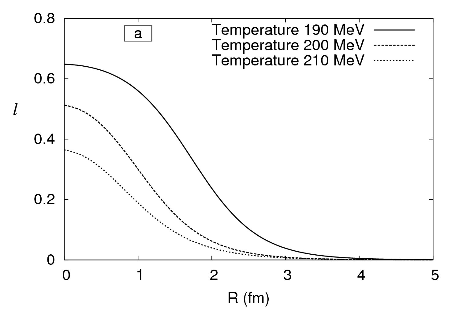
Figure 2:

(a) Critical bubble profiles for different values of the temperature. (b) Solid curve shows the critical bubble for the 3+1 dimensional case (which for finite temperature case becomes 3 Euclidean dimensional) for $T$ = 200 MeV and the dotted curve shows the same for 2+1 dimensional case (i.e. 2 Euclidean dimensions for finite temperature case).

Recall that we are calculating bubble profiles using Eq.(7) relevant for the 3+1 dimensional case, however, the field evolution is done using 2+1 dimensional equations as appropriate for the mid rapidity region of rapidly longitudinally expanding plasma. In Fig.(2b) solid curve shows the critical bubble for the 3+1 dimensional case (which for finite temperature case becomes 3 Euclidean dimensional) for $T$ = 200 MeV and the dashed curve shows the same for 2+1 dimensional case (i.e. 2 Euclidean dimensions for finite temperature case). It is clear that the 3 dimensional bubble is of supercritical size and will expand when evolved with 2+1 dimensional equations. This avoids the artificial construction of suitable supercritical bubbles which can expand and coalesce as was done in ref.ajit . (Recall that for the finite temperature case, a bubble of exact critical size will remain static when evolved by the field equations. In a phase transition, bubbles with somewhat larger size than the critical size expand, while those with smaller size contract.)

For the bubble profile given by the solid curve in Fig.(2b), the value of the action $S_{3}(l)$ is about 240 MeV. Using Eq.(6) for the nucleation rate, we find that the nucleation rate of QGP bubbles per unit time per unit volume is of the order of $0.025fm^{-4}$. The thermalization time for QGP phase is of the order of 1 fm at RHIC (say, for Au-Au collision at 200 GeV energy). Hence the time available for the nucleation of QGP bubbles is at most about 1 fm. We take the region of bubble nucleation to be of thick disk shape with the radius of the disk (in the transverse direction) of about 8 fm and the thickness of the disk (in the longitudinal direction) of about 1 fm. Total space-time volume available for bubble nucleation is then about 200 fm⁴ (in practice, less than this). For the case of Eq.(6), net number of bubbles is then equal to 5.

For the case of the nucleation rate given by Eq.(10), one needs an estimate of the critical bubble size $R_{c}$ as well as bubble surface energy $\sigma$, (along with other quantities like $\lambda$ etc. as given by Eqs.(11)-(14)). Determination of $R_{c}$ is somewhat ambiguous here as the relevant bubbles are thick wall bubbles as seen in Fig.(2). Here there is no clear demarcation between the core region and the surface region which could give an estimate of $R_{c}$. Essentially, there is no core at all and the whole bubble is characterized by the overlap of bubble wall region. We can take, as an estimate for the bubble radius $R_{c}$ any value from 1 fm - 1.5 fm. It is important to note here that this estimate of $R_{c}$ is only for the calculation of nucleation rate $\Gamma$, and not for using the bubble profile for actual simulation. When bubbles are nucleated in the background of false vacuum with $l=0$, a reasonably larger size of the bubble is used so that cutting off the profile at that radius does not lead to computational errors and field evolution remains smooth.

Once we have an estimate of $R_{c}$, we can then estimate the surface tension $\sigma$ (which also is not unambiguous here) as follows. With the realization that essentially there is no core region for the bubbles in Fig(2), we say that the entire energy of the bubble (i.e. the value of $S_{3}$) comes from the surface energy. Then we write

$$4\pi R_{c}^{2}\sigma=S_{3}$$ (15)

For $S_{3}$ = 240 MeV, we get $\sigma=8$ MeV/fm² if we take $R_{c}$ = 1.5 fm. With $R_{c}$ = 1.0 fm, we get $\sigma$ = 20 MeV/fm².

Number of bubbles expected can now be calculated for the case when nucleation rate is given by Eq.(10). We find number of bubbles to be about 10^-4 with $R_{c}$ taken as 1.5 fm. This is in accordance with the results discussed in ref. kpst . The bubble number increases by about a factor 5 if $R_{c}$ is taken to be about 1 fm. Thus, with the estimates based on Eq.(10), bubble nucleation is a rare event for the time available for RHICE.

As we have mentioned above, for us the bubble nucleation on one hand represents the possibility of actual dynamics of a first order transition, while on the other hand, it represents the generic properties of the domain structure arising from a C-D transition, which may very well be a cross-over, occurring in a finite time. With this view, and with various uncertainties in the determination of pre-exponential factors in the nucleation rate, we will consider a larger number of bubbles also and study domain wall and string production. First we will consider nucleation of 5 bubbles and then we will consider nucleation of 9 bubbles to get a better network of domain walls and strings.

V NUMERICAL TECHNIQUES

In our simulation critical bubbles are nucleated at a time when the temperature $T$ crosses the value $T=200$ MeV during the initial stage between $\tau=0$ to $\tau=\tau_{0}=1$ fm (during which we have modeled the system temperature to increase linearly from 0 to $T_{0}$). We take $T_{0}=400$ MeV so bubble nucleation stage is taken to be at $\tau=0.5$ fm when $T$ reaches the value 200 MeV. Again, this is an approximation since in realistic case bubbles will nucleate over a span of time given by the (time dependent) nucleation rate, which could lead to a spectrum of sizes of expanding bubbles at a given time. However, due to very short time available to complete the nucleation of QGP bubbles in the background of confined phase, bubbles will have very little time to expand during the nucleation period of all bubbles (especially as initial bubble expansion velocity is zero). Thus it is reasonable to assume that all the bubbles nucleate at the same time.

After nucleation, bubbles are evolved by the time dependent equations of motion in the Minkowski space rndrp as appropriate for Bjorken’s longitudinal scaling model.

$${\ddot{l}_{i}}+{{\dot{l}_{i}}\over\tau}-{\partial^{2}l_{i}\over\partial x^{2}}-{\partial^{2}l_{i}\over\partial y^{2}}={-\partial V(l)\over{\partial l_{i}}},\qquad i=1,2$$ (16)

with ${\dot{l}}=0$ at $\tau$ = 0. Here $l=l_{1}+il_{2}$, and dot indicates derivative with respect to the proper time $\tau$.

The bubble evolution was numerically implemented by a stabilized leapfrog algorithm of second order accuracy both in space and in time with the second order derivatives of $l_{i}$ approximated by a diamond shaped grid. Here we follow the approach described in ajit to simulate the first order transition. We need to nucleate several bubbles randomly choosing the corresponding Z(3) vacua for each bubble. This is done by randomly choosing the location of the center of each bubble with some specified probability per unit time per unit volume. Before nucleating a bubble, it is checked if the relevant region is in the false vacuum (i.e. it does not overlap with some other bubble already nucleated). In case there is an overlap, the nucleation of the new bubble is skipped. The orientation of $l$ inside each bubble is taken to randomly vary between the three Z(3) vacua.

For representing the situation of relativistic heavy ion collision experiments, the simulation of the phase transition is carried out by nucleating bubbles on a square lattice with physical size of 16 fm within a circular boundary (roughly the Gold nucleus size). We use fixed boundary condition, free boundary condition, as well as periodic boundary condition for the square lattice. To minimize the effects of boundary (reflections for fixed boundary, mirror reflections for periodic boundary conditions), we present results for free boundary conditions (for other cases, the qualitative aspects of our results remain unchanged). Even for free boundary conditions, spurious partial reflections occur, and to minimize these effects we use a thin strip (of 10 lattice points) near each boundary where extra dissipation is introduced.

We use 2000 $\times$ 2000 lattice. For the physical size of 16 fm, we have $\Delta x$ = 0.008 fm. To satisfy the Courant stability criteria, we use $\Delta t=\Delta x/\sqrt{2}$, as well as $\Delta t=0.9\Delta x/\sqrt{2}$, (which we use for the results presented in the paper). For Au-Au collision at 200 GeV, the thermalization is expected to happen within 1 fm time. As mentioned above, in this pre-equilibrium stage, we model the system as being in a quasi-equilibrium stage with a temperature which increases linearly with time (for simplicity). The temperature of the system is taken to reach upto 400 MeV in 1 fm time, starting from $T$ = 0. After $\tau=\tau_{0}=1$ fm, the temperature decreases due to continued longitudinal expansion, i.e.

$$T(\tau)=T(\tau_{0})\left({\tau_{0}\over\tau}\right)^{1/3}$$ (17)

The stability of the simulation is checked by checking the variation of total energy of the system during the evolution. The energy fluctuation remains within few percent, with no net increase or decrease in the energy (for fixed and periodic boundary conditions, and without the dissipative $\dot{l}$ term in Eq.(16)) showing the stability of the simulation.

The bubbles grow and eventually start coalescing, leading to a domain like structure. Domain walls are formed between regions corresponding to different Z(3) vacua, and strings form at junctions of Z(3) domain walls. Recall that the domain wall network is formed here in the transverse plane, appearing as curves. These are the cross-sections of the walls which are formed by elongation (stretching) of these curves in the longitudinal direction into sheets. At the intersection of these walls, strings form. In the transverse plane, these strings looks like vortices, which will be elongated into strings in the longitudinal direction.

VI Effects of quarks

We now discuss the effects of quarks. As we mentioned above, we will follow the approach where the presence of quarks is interpreted as leading to explicit breaking of the Z(3) symmetry, lifting the degeneracy of different Z(3) vacua qurk2 ; psrsk ; psrsk2 . This has important effects in the context of our model. First of all, different vacua having different energies implies different nucleation rates for the QGP bubbles with different Z(3) vacua. Further, for non-degenerate vacua, even planar $Z(3)$ interfaces do not remain static, and move away from the region with the unique true vacuum. Thus, while for the degenerate vacua case every closed domain wall collapses, for the non-degenerate case this is not true any more. A closed wall enclosing the true vacuum may expand if it is large enough so that the surface energy contribution does not dominate (this is essentially the same argument as given for the bubble expansion, see Eq.(5) and the discussion following it).

To see the importance of these effects we need an estimate of the explicit symmetry breaking term arising from inclusion of quarks. For this we use the estimates given in prsr ; z3lnr . Even though the estimates in ref.prsr are given in the high temperature limit, we will use these for temperatures relevant for our case, i.e. $T\simeq 200-400$ MeV, to get some idea of the effects of the explicit symmetry breaking. The difference in the potential energy between the true vacuum with $l=1$ and the other two vacua ($l=e^{i2\pi/3}$, and $l=e^{i4\pi/3}$, which are degenerate with each other) is estimated in ref. prsr to be,

$$\Delta V\sim{2\over 3}\pi^{2}T^{4}{N_{l}\over N^{3}}(N^{2}-2)$$ (18)

where $N_{l}$ is the number of massless quarks. If we take $N_{l}=2$ then $\Delta V\simeq 3T^{4}$. At the bubble nucleation temperature (which we have taken to be about $T=200$ MeV, the difference between the false vacuum and the true vacuum is about 150 MeV/fm³ while $\Delta V$ at $T=200$ MeV is about four times larger, equal to 600 MeV/fm³. As $T$ approaches $T_{c}$, this difference will become larger as the metastable vacuum and the stable vacuum become degenerate at $T_{c}$, while $\Delta V$ remains non-zero. For $T$ near 250 MeV (where the barrier between the metastable vacuum and the stable vacuum disappears), $\Delta V$ becomes almost comparable to the difference between the potential energy of the false vacuum (the confining vacuum) and the true vacuum (deconfined vacuum).

It does not seem reasonable that at temperatures of order 200 MeV a QGP phase (with quarks) has higher free energy than the hadronic phase. This situation can be avoided if the estimates of Eq.(18) are lowered by about a factor of 5 so that these phases have lower free energy than the confining phase. (A more desirable situation will be when $\Delta V$ approaches zero as the confining vacuum and the deconfining (true) vacuum become degenerate at $T_{c}$.) It is in the spirit of the expectation that explicit breaking of Z(3) is small near $T_{c}$ for finite pion mass z3lnr . Even with such lower estimates, the effects of quarks may give different nucleation probabilities for different Z(3) vacua. However, in this paper we will ignore this possibility. This may not be very unreasonable as for thick wall bubbles thermal fluctuations may be dominant in determining the small number of bubbles nucleated during the short span of time available. For very few bubbles nucleated, there may be a good fraction of events where different Z(3) vacua may occur in good fraction. Also note that the pre-exponential factor for the bubble nucleation rate of Eq.(6), as given in Eq.(9) increases with the value of $S_{3}(l)$. Thus, for the range of values of $S_{3}(l)$ for which the exponential factor in Eq.(6) is of order 1, which is likely in our case, the nucleation rate may not decrease with larger values of $S_{3}(l)$, i.e. for the Z(3) vacua with higher potential energies than the true vacuum. (Of course for very large values of $S_{3}(l)$ the exponential term will suppress the nucleation rate.) Thus our assumption of neglecting quark effects for the bubble nucleation rate may not be unreasonable.

We now consider the effect of non-zero $\Delta V$, as in Eq.(18), on the evolution of closed domain walls. The temperature range relevant for our case is $T=200-400$ MeV. In an earlier work we had numerically estimated the surface tension of Z(3) walls to be about 0.34 and 7.0 GeV/fm² for $T$ = 200 and 400 MeV respectively. The effects of quarks will be significant if a closed spherical wall (with true vacuum inside) starts expanding instead of collapsing. Again, using the bubble free energy Eq.(5), with $\eta=\Delta V$ and $\sigma$ as the surface energy of the interface, we see that the critical radius $R^{*}$ of the spherical wall is

$$R^{*}={2\sigma\over\eta}\simeq 2\sigma/3T^{4}$$ (19)

For $T$ = 200 MeV and 400 MeV we get $R^{*}\simeq 1$ and 1.5 fm respectively. Though these values are not large, these are not too small either when considering the fact that relevant sizes and times for RHICE are of order few fm anyway. The values of $R^{*}$ we estimated here are very crude as for these sizes wall thickness is comparable to $R^{*}$ hence application of Eq.(5), separating volume and surface energy contributions, is not appropriate. Further, as we discussed above, the estimate in Eq.(18) which is applicable for high temperature limit, seems an over estimate by about an order of magnitude at these temperatures. Thus uncertainties of factors of order 1 may not be unreasonable to expect. In that case the dynamics of closed domain walls of even several fm diameter will not be affected by the effects of quarks via Eq.(18).

We will see in the next section of simulation results that the domain walls and strings typically have large velocities (e.g. about 0.5 - 0.8) at the time of formation. These result from momentum of colliding bubble walls and from curvature in the shape of these walls (as well as asymmetries in the profiles of strings) at the time of formation. With such large velocities present, the effects of pressure differences between different Z(3) vacua due to quarks may become subdominant in studying the evolution of these structures for the short time duration available for RHICE.

With this, we will assume that for small closed walls, of order few fm diameter, as is expected in RHICE, the quark effects in the evolution of wall network may be neglected. We plan to remove these assumptions and include the effects of non-zero $\Delta V$ due to quarks on bubble nucleation and wall evolution in a future work.

VII RESULTS OF THE SIMULATION

As we mentioned above, the number of bubbles expected to form in RHICE is small. We first present and discuss the case of 5 bubbles which is more realistic from the point of view of nucleation estimates given by Eq.(6) (though a gross over-estimate for Eq.(10)). Note that a domain wall will form even if only two bubbles nucleate (with different Z(3) vacua). However, to see QGP string formation, we need nucleation of at least three bubbles. Next we will discuss the case of 9 bubbles which is a much more optimistic estimate of the nucleation rate (even for Eq.(6)). Alternatively, this case can be taken as better representation of the case when the transition is a cross over and bubbles only represent a means for developing a domain structure expected after the cross-over is completed. (In this case only relevant energy density fluctuations, as discussed below, will be those arising from Z(3) walls and strings, and not the ones resulting from bubble wall coalescence.)

VII.1 formation and motion of extended walls

Fig.3-7 show the results of simulation when five bubbles are nucleated with random choices of different Z(3) vacua inside each bubble. Fig.3 shows a time sequence of surface plots of the order parameter $l(x)$ in the two dimensional lattice. Fig.3a shows the initial profiles of the bubbles of the QGP phase embedded in the confining vacuum with $l=0$ at $\tau$ = 0.5 fm with the temperature $T=$ 200 MeV. (Recall that for initial 1 fm time the temperature is taken to linearly increase from zero to $T_{0}$ = 400 MeV.) The radial profile of each bubble is truncated with appropriate care of smoothness on the lattice for proper time evolution. Fig.3b shows the profile of each bubble at $\tau=$ 1.5 fm showing the expansion of the bubbles. Near the outer region of a bubble the field grows more quickly towards the true vacuum. If bubbles expand for long time then bubble walls become ultra-relativistic and undergo large Lorentz contraction. This causes problem in simulation (see, e.g. ajit ). In our case this situation arises at outer boundaries (for the inner regions bubbles collide quickly). For outer regions also it does not cause serious problem because of the use of dissipative boundary strip (as explained above in Sect.V).

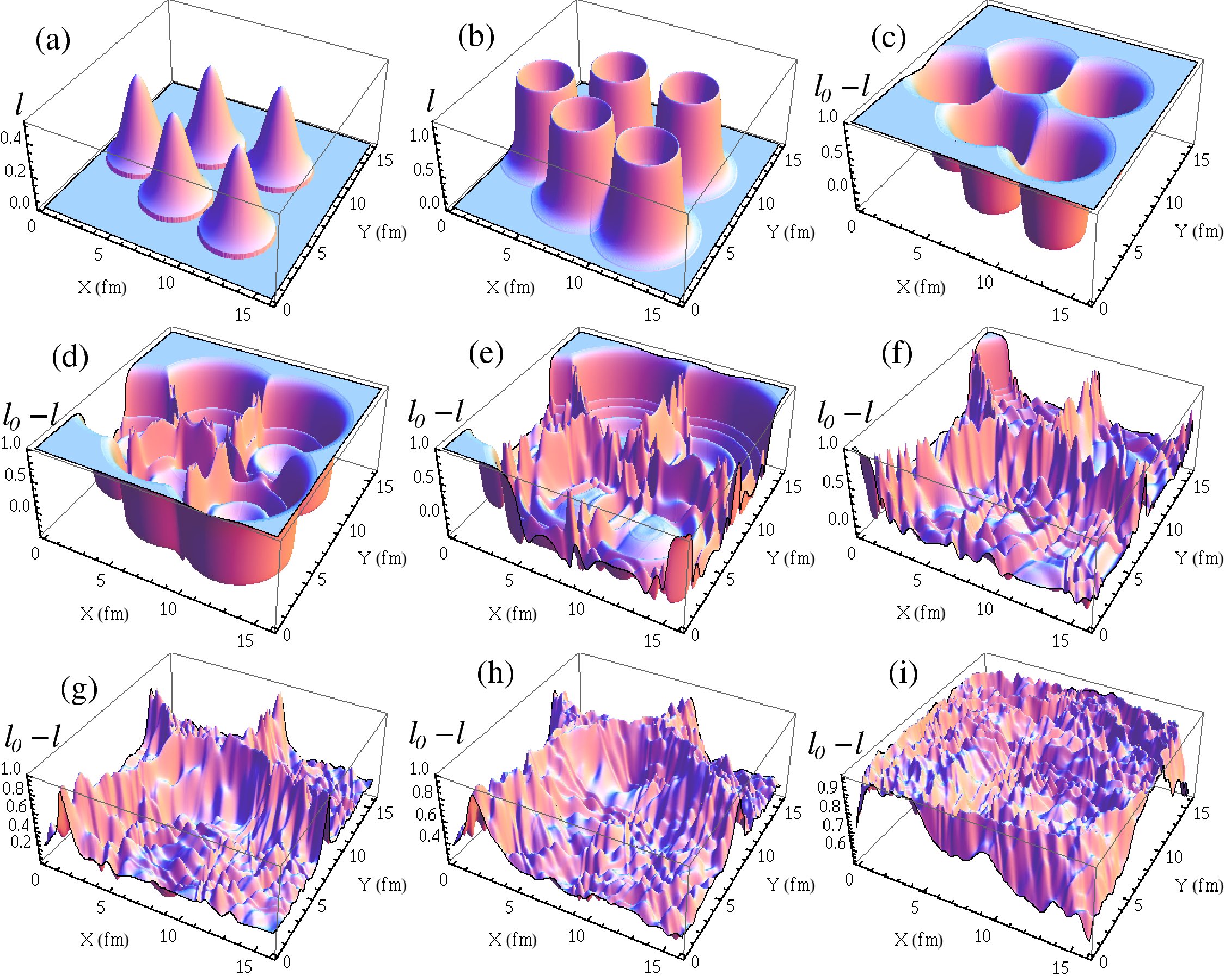
Figure 3:

(a) and (b) show plots of profiles of $l$ at $\tau=$ 0.5 fm and 1.5 fm respectively. (c)-(i) show plots of $l_{0}-l$ at $\tau=$ 1.5, 2.5, 4.0, 6.0, 9.0, 11.0, and 13.7 fm. $T$ drops to below $T_{c}$ around at $\tau=$ 10.5 fm and $T=$ 167 MeV at $\tau=$ 13.7 fm. Formation of domain walls and string and antistring (at junctions of three walls) can be seen in the plots in (e) - (h).

Figs. 3c-3i show plots of $l_{0}-l$ clearly showing formation of domain walls and strings (junctions of three walls). Here $l_{0}$ is a reference vacuum expectation value of $l$ calculated at the maximum temperature $T=T_{0}=$ 400 MeV. Formation of domain walls, extending through the entire QGP region, is directly visible from Fig.3e (at $\tau=4$ fm) onwards. The temperature drops to below $Tc\simeq 182$ MeV at $\tau\simeq 10.5$ fm. The last plot in Fig.3i is at $\tau=13.7$ fm when the temperature $T=$ 167 MeV, clearly showing that the domain walls have decayed away in the confined phase and the field is fluctuating about $l=0$.

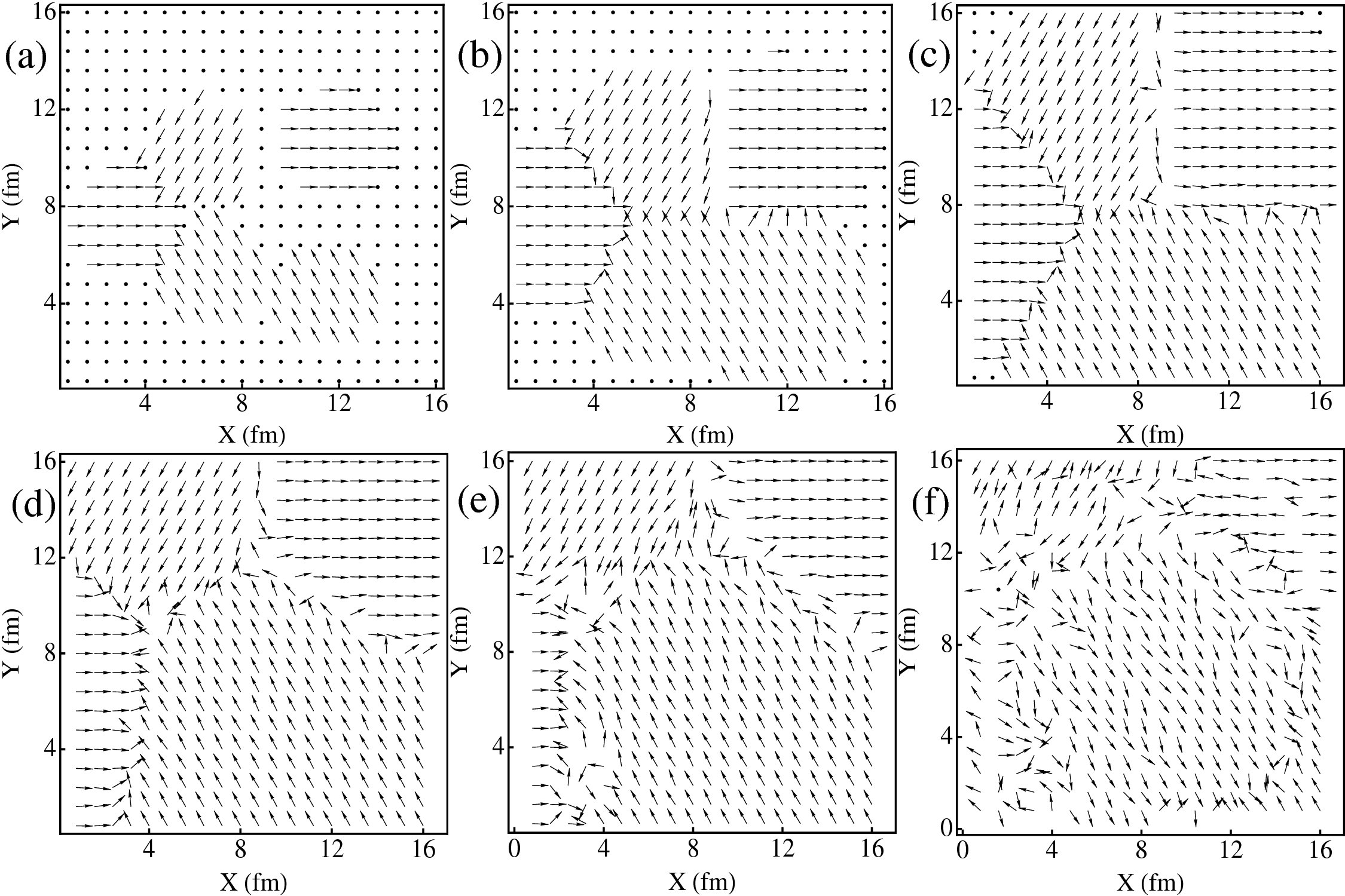
Figure 4:

Plots of the phase $\theta$ of the order parameter $l$. (a) shows the initial distribution of $\theta$ in the bubbles at $\tau=$ 0.5 fm. (b) - (f) show plots of $\theta$ at $\tau=$ 2.0, 4.6, 11.0, 12.2, and 13.7 fm respectively. Location of domain walls and the string (with positive winding) and antistring (with negative winding) are clearly seen in the plots in (b)-(e). The motion of the antistring and associated walls can be directly seen from these plots and an estimate of the velocity can be obtained.

In Fig.3f-3h we see two junctions of three domain walls where the QGP strings form. This is seen more clearly in Fig.4 where the phase $\theta$ of $l$ is plotted (with the convention that $\theta$ is the angle of the arrow from the positive $X$ axis). The domain walls are identified as the boundaries where two different values of $\theta$ meet, and strings correspond to the non-trivial winding of $\theta$ at the junctions of three walls. From Fig.4b,c we clearly see that at one of the junctions we have a string (at $X\simeq$ 5 fm, $Y\simeq$ 8 fm) with positive winding and we have an anti-string at $X\simeq$ 9 fm, $Y\simeq$ 8 fm with negative winding. Note the rapid motion of the walls forming the antistring towards positive $Y$ axis from Fig.4c (at $\tau=$ 4.6 fm) to Fig.4e (at $\tau=$ 12.2 fm). The average speed of the antistring (and wall associated with that) can be directly estimated from these figures to be about 0.5 (in natural units with $c=1$). This result is important in view of the discussion in the preceding section showing that effects of pressure differences between different Z(3) vacua, arising from quarks, may be dominated by such random velocities present for the walls and strings at the time of formation. The motion of the walls here is a direct result of the straightening of the $L$ shaped wall structure due to its surface tension. For the same reason the wall in the left part of Fig.4b also straightens from the initial wedge shape. Fig.4f shows almost random variations of $\theta$ at $\tau=13.7$ fm when the temperature is 167 MeV, well below the critical temperature. Though it is interesting to note that a large region of roughly uniform values of $\theta$ still survives at this stage.

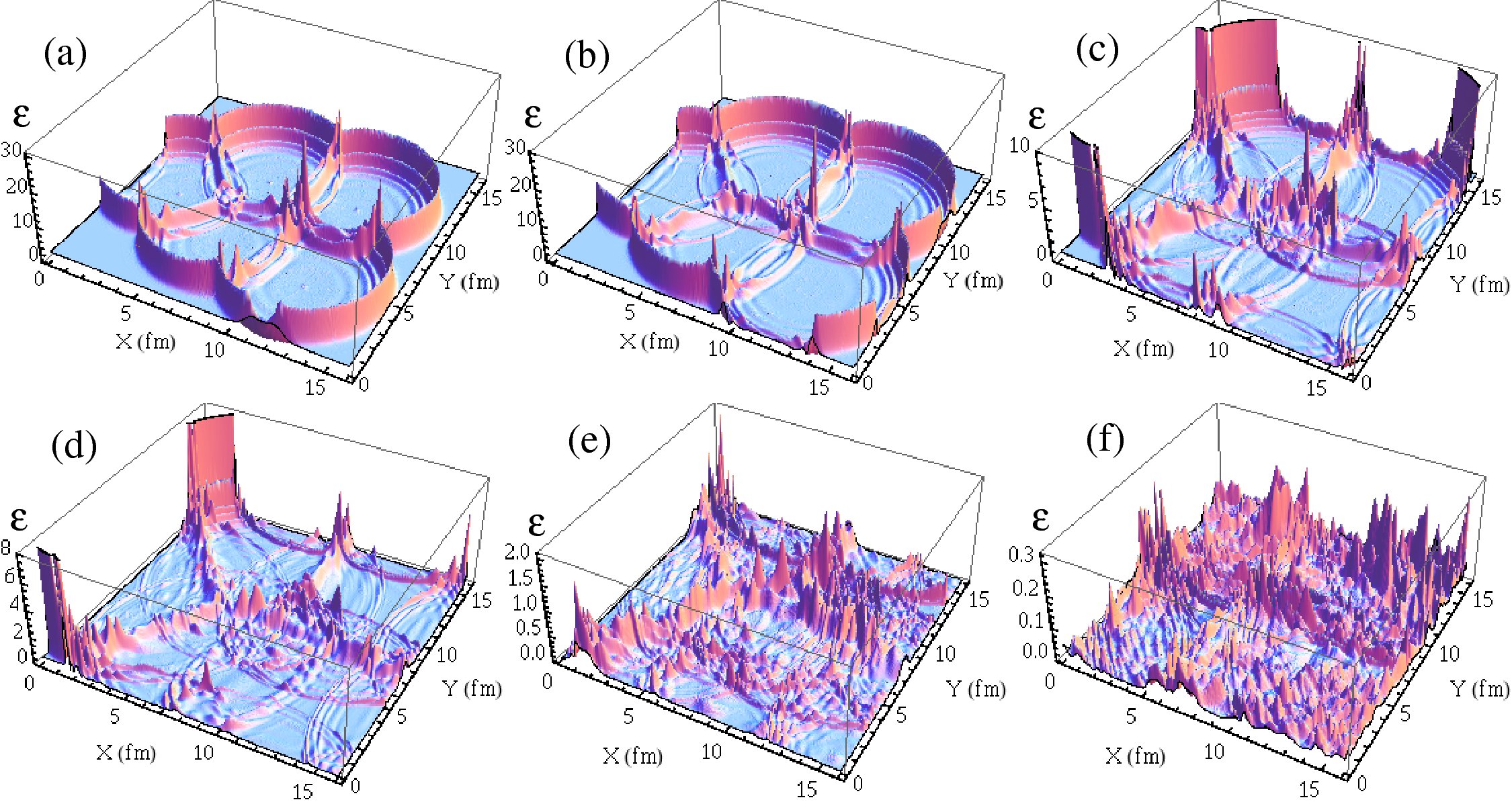
Figure 5:

Surface plots of the local energy density ${\varepsilon}$ in GeV/fm³. (a) - (f) show plots at $\tau=$ 3.0, 3.6, 5.0, 6.0, 8.0, and 13.2 fm respectively. Extended domain walls can be seen from these plots of $\varepsilon$ in (b) - (e). Small peaks in $\varepsilon$ exist at the locations of string and antistring (larger peaks arise from oscillations of field where bubbles coalesce). Plot in (f) is at the stage when $T=$ 169 MeV and domain walls have decayed away.

Fig.5 shows surface plots of the local energy density $\varepsilon$. $\varepsilon$ is plotted in units of GeV/fm³. Although the simulation is 2+1 dimensional representing the transverse plane of the QGP system, we calculate energy in 3+1 dimensions by taking a thickness of 1 fm in the central rapidity region. Fig.5a shows plot at $\tau=$ 3 fm when bubbles have coalesced. In Fig.5b at $\tau=$ 3.6 fm we see that bubble walls have almost decayed (in ripples of $l$ waves) between the bubbles with same $\theta$ (i.e. same Z(3) vacua) as can be checked from $\theta$ plots in Fig.4. Energy density remains well localized in the regions where domain walls exist. Also, one can see the small peaks in the energy density where strings and antistrings exist. Large peaks arise from oscillations of $l$ when bubble walls coalesce, as discussed in ajit . Large values of $\varepsilon$ near the boundary of the lattice are due to relativistically expanding bubble walls. Motion of walls and generation of increased fluctuations in energy density are seen in Fig.5c-5e. Fig.5f at $\tau=$ 13.2 fm (with $T$ = 169 MeV) shows that walls have decayed. However, some extended regions of high energy density can be seen at this stage also.

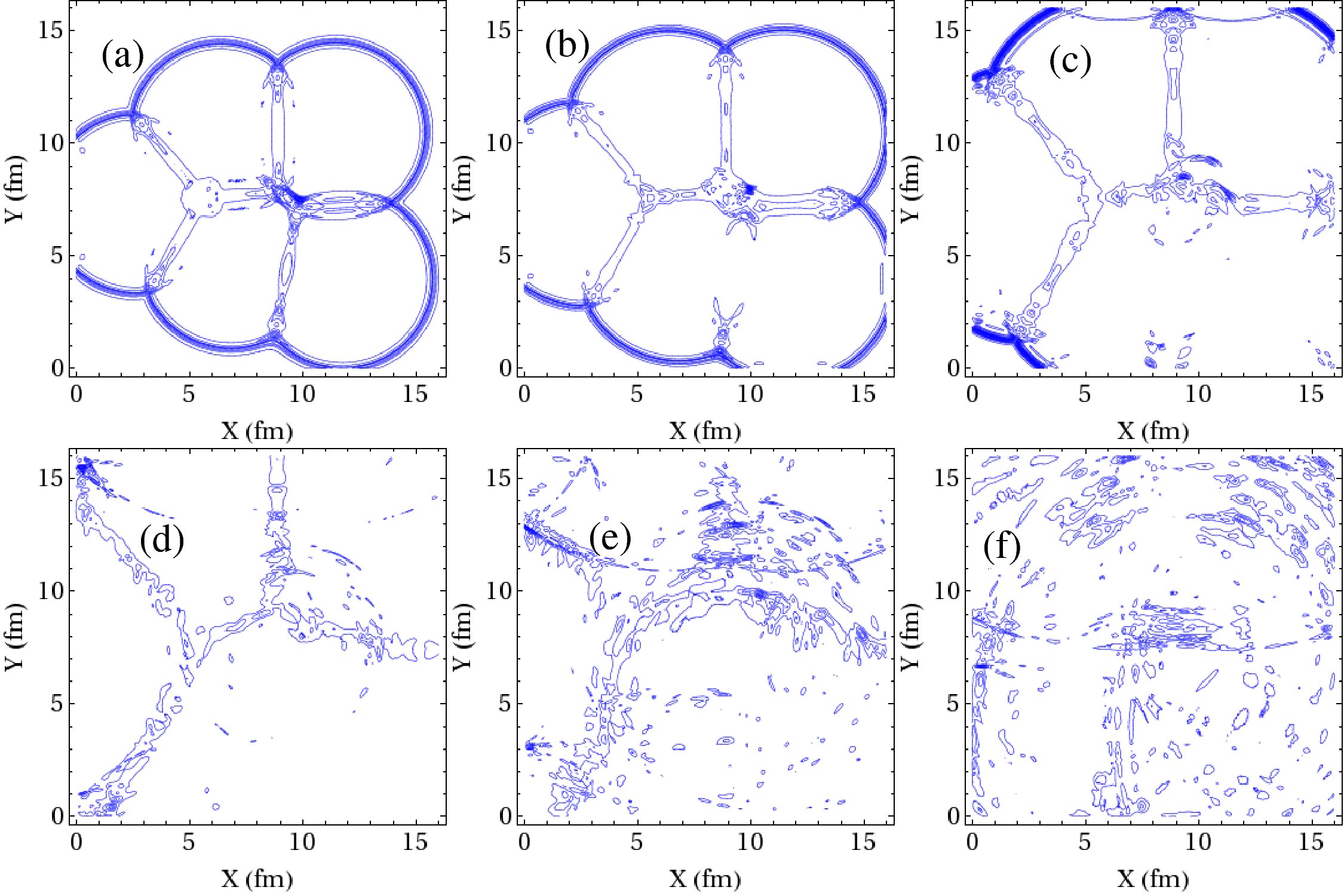
Figure 6:

Contour plots of the local energy density $\varepsilon$ at different stages. Plots in (a) - (f) correspond to $\tau=$ 3.0, 3.6, 5.0, 7.6, 10.2, and 13.2 fm respectively. Structure of domains walls formed near the coalescence region of bubbles with different $\theta$ is clear in (b), whereas the bubble walls at lower half of $Y$ region, and near $X=$ 10 fm, are seen to simply decay away due to same vacuum in the colliding bubbles. Motion of the antistring and associated domain walls is clear from plots in (b) - (e). The last plot in (f) is at $\tau=13.2$ fm when $T$ = 169 MeV.

Fig.6 shows contour plots of energy density $\varepsilon$. Fig.6a shows coalescence of bubbles at $\tau=$ 3 fm. Fig.6b at $\tau=$ 3.6 fm clearly shows the difference in the wall coalescence depending on the vacua in the colliding bubbles. Where domain walls exist, we see extended regions of high energy density contours whereas where the two vacua in colliding bubbles are same, there are essentially no high energy density contours. Motion of domain walls (and strings at wall junctions) is clearly seen in these contour plots in Fig.6b-6d. Fig.6e is at $\tau=$ 10.2 fm when $T$ drops to $T_{c}$. Wall structures are still present. Fig.6f is at $\tau=$ 13.2 fm ($T$ = 169 MeV) when walls have decayed away, though some extended structures in contours still survive.

We have also calculated the variance of energy density $\Delta\varepsilon$ at each time stage to study how energy fluctuations change during the evolution. In Fig.7 we show the plot of $\Delta\varepsilon/\varepsilon$ as a function of proper time. Here $\varepsilon$ is the average value of energy density at that time stage. The energy density $\varepsilon$ decreases due to longitudinal expansion, hence we plot this ratio to get an idea of relative importance of energy density fluctuations. Fig.7 shows initial rapid drop in $\Delta\varepsilon/\varepsilon$ due to large increase in $\varepsilon$ during the heating stage upto $\tau$ = 1 fm, followed by a rise due to increased energy density fluctuations during the stage when bubbles coalesce and bubble walls decay, as expected. Interesting thing to note is a slight peak in the plot near $\tau=$ 10.5 fm when $T$ drops below $T_{c}$. This should correspond to the decay of domain walls and may provide a signal for the formation and subsequent decay of such objects in RHICE.

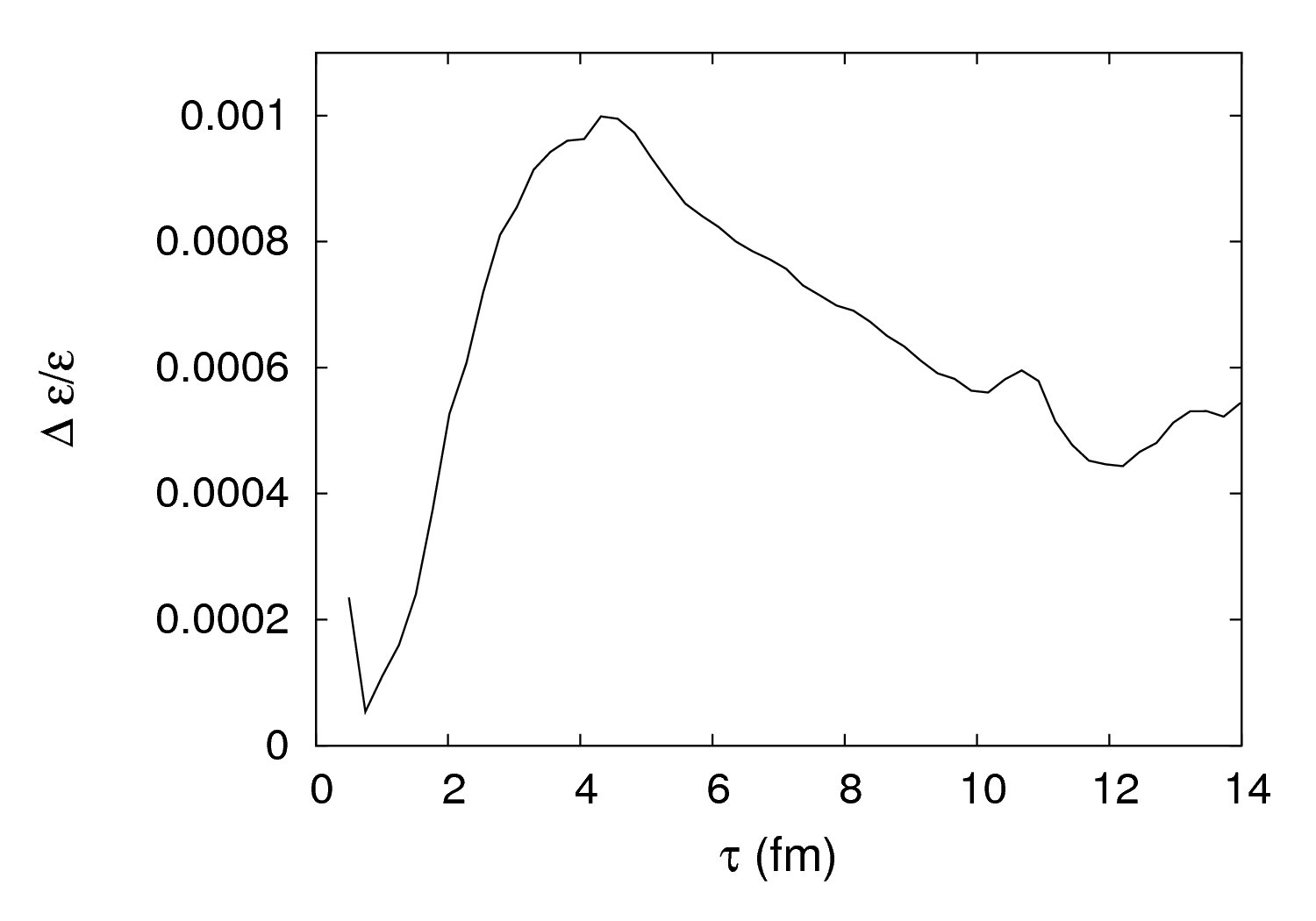
Figure 7:

Plot of the ratio of variance of energy density $\Delta\varepsilon$ and the average energy density $\varepsilon$ as a function of proper time. Energy fluctuations increase during the initial stages when bubbles coalesce and bubble walls decay. After that there is a slow decrease in energy fluctuation until the stage when the temperature drops below $T_{c}$ and $\tau\simeq 10.5$ fm. Energy fluctuations increase after this stage. Note small peak near the transition stage.

VII.2 Formation and collapse of a closed wall

Fig.8-12 show the results of simulation where nine bubbles are nucleated. Fig.8 shows a time sequence of surface plots of $l(x)$ (similar to Fig.3). Fig.8a shows the initial profiles of the QGP bubbles at $\tau$ = 0.5 fm with the nucleation temperature of $T=$ 200 MeV. Fig.8b shows the profile of $l$ for the bubbles at $\tau=$ 1.5 fm showing the expansion of the bubbles. Fig.8c-8i show plots of $l_{0}-l$ at different stages. Noteworthy here is the formation of a closed domain wall near the central region which is clearly first seen in Fig.8e at $\tau=$ 5 fm. The collapse of this closed domain wall is seen in the subsequent plots with the closed wall completely collapsing away in Fig.8h at $\tau=$ 9.6 fm. Only surviving structure is an extended domain wall along the $X$ axis. Fig.8i is at $\tau=13.2$ fm when $T=$ 169 MeV. The domain walls have decayed away and $l$ fluctuates about the value zero as appropriate for the confined phase.

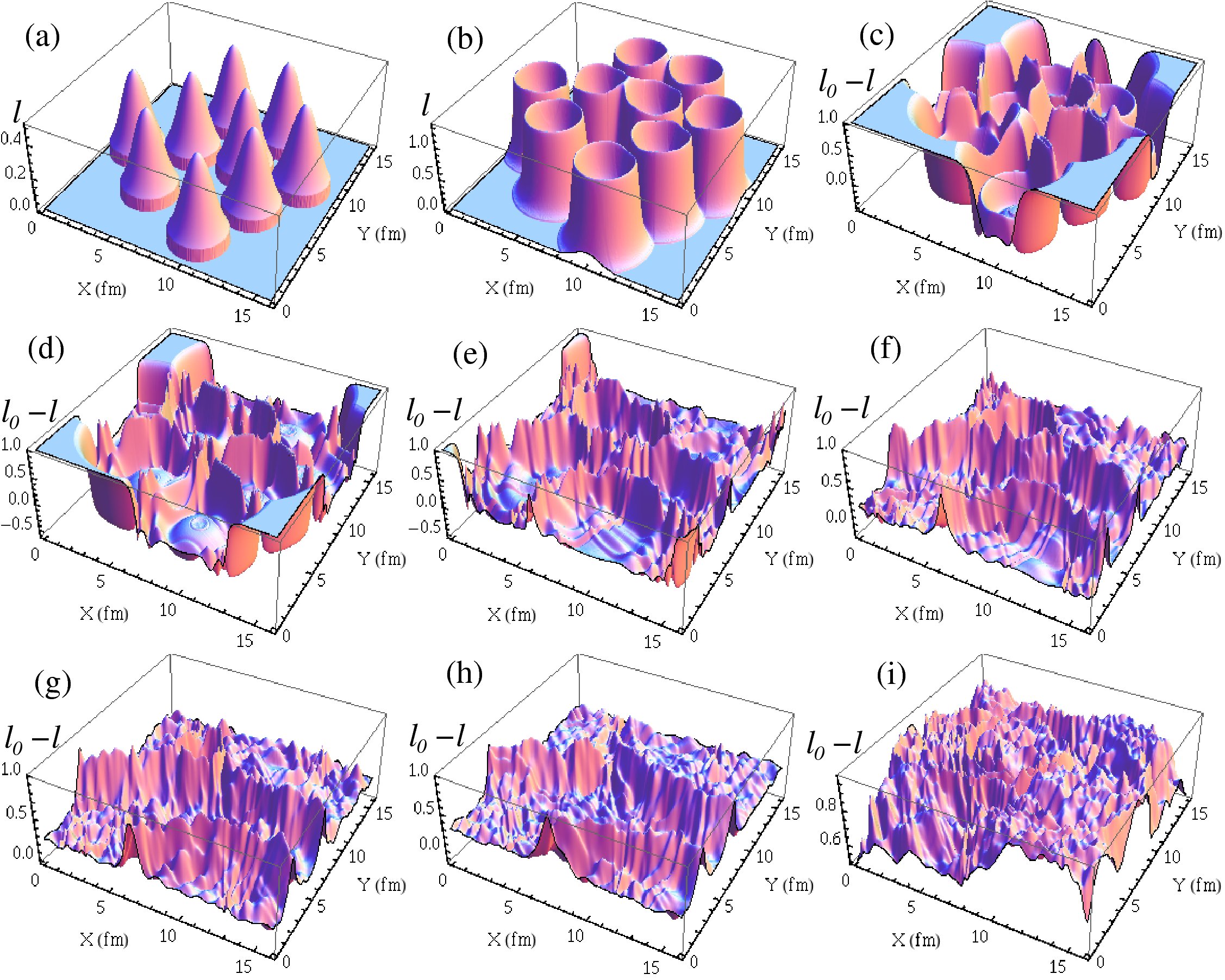
Figure 8:

(a) and (b) show plots of profiles of $l$ at $\tau=$ 0.5 fm and 1.5 fm respectively for the case when 9 bubbles are nucleated. (c)-(i) show plots of $l_{0}-l$ at $\tau=$ 2.0, 3.0, 5.0, 7.0, 8.6, 9.6, and 13.2 fm respectively. Formation of a closed domain wall is first clearly seen in the plot in (e). This closed domain wall collapses as seen in plots in (e) through (h). Only surviving domain wall is an extended wall along $X$ axis in (h). Plot in (i) is when the temperature $T=$ 169 MeV.

Fig.9 shows plots of the phase $\theta$ of $l$ at different stages. Initial phase distribution in different bubbles is shown in Fig.9a at $\tau=0.5$ fm. Fig.9b shows the formation of closed, elliptical shaped domain wall at $\tau=2.6$ fm. Strings and antistrings can also be identified by checking the windings of $\theta$. The closed domain wall collapses, and in the process becomes more circular, as shown in the plots in Fig.9b-9h. Fig.9h shows the plot at $\tau=$ 9.6 fm when the closed domain wall completely collapses away, leaving only an extended domain wall running along $X$ axis between $Y\simeq 4-8$ fm. The final Fig.9i at $\tau=13.8$ fm is when the temperature $T=$ 167 MeV showing random fluctuations of $\theta$ when domain walls have decayed away in the confining phase.

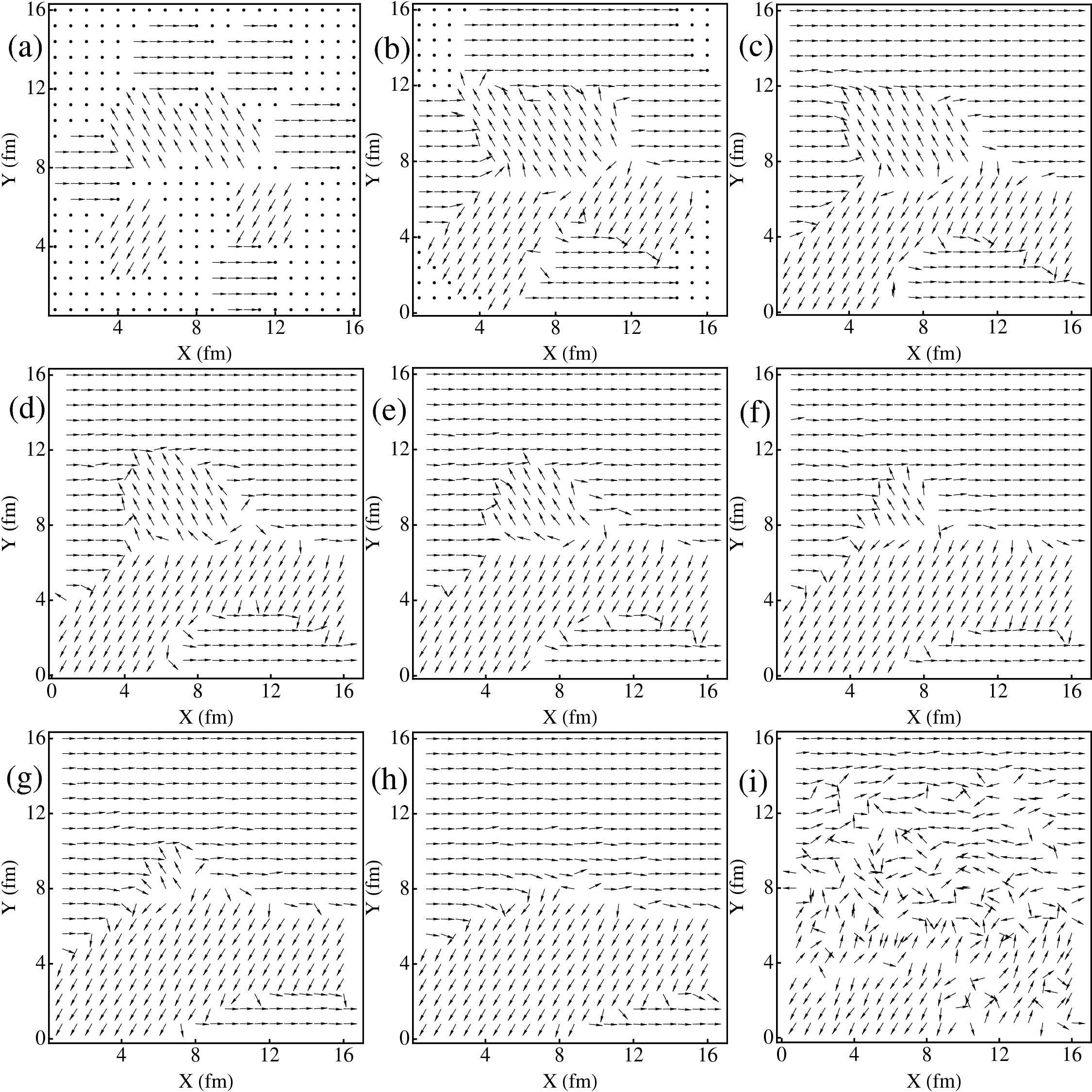
Figure 9:

Plots of the phase $\theta$ of $l$. (a) shows initial distribution of $\theta$ in the bubbles at $\tau=$ 0.5 fm. (b) - (i) show plots of $\theta$ at $\tau=$ 2.6, 5.0, 6.0, 7.0, 8.0, 8.6, 9.6, and 13.8 fm respectively. (b) shows formation of elliptical shaped closed domain wall which subsequently becomes more circular as it collapses away by $\tau=$ 9.6 fm as shown by the plot in (h). The plot in (i) is at $T=167$ MeV showing random fluctuations of $\theta$.

Fig.10 shows the surface plot of energy density $\varepsilon$ at different stages. Extended thin regions of large values of $\varepsilon$ are clearly seen in the plots corresponding to domain walls. Collapse of the closed domain wall is also clearly seen in Fig.10c-10g. Important thing to note here is the surviving peak in the energy density plot at the location of domain wall collapse. This peak survives even at the stage shown in Fig.10i at $\tau=13.2$ fm when $T=169$ MeV, well below the transition temperature. Such hot spots may be the clearest signals of formation and collapse of Z(3) walls.

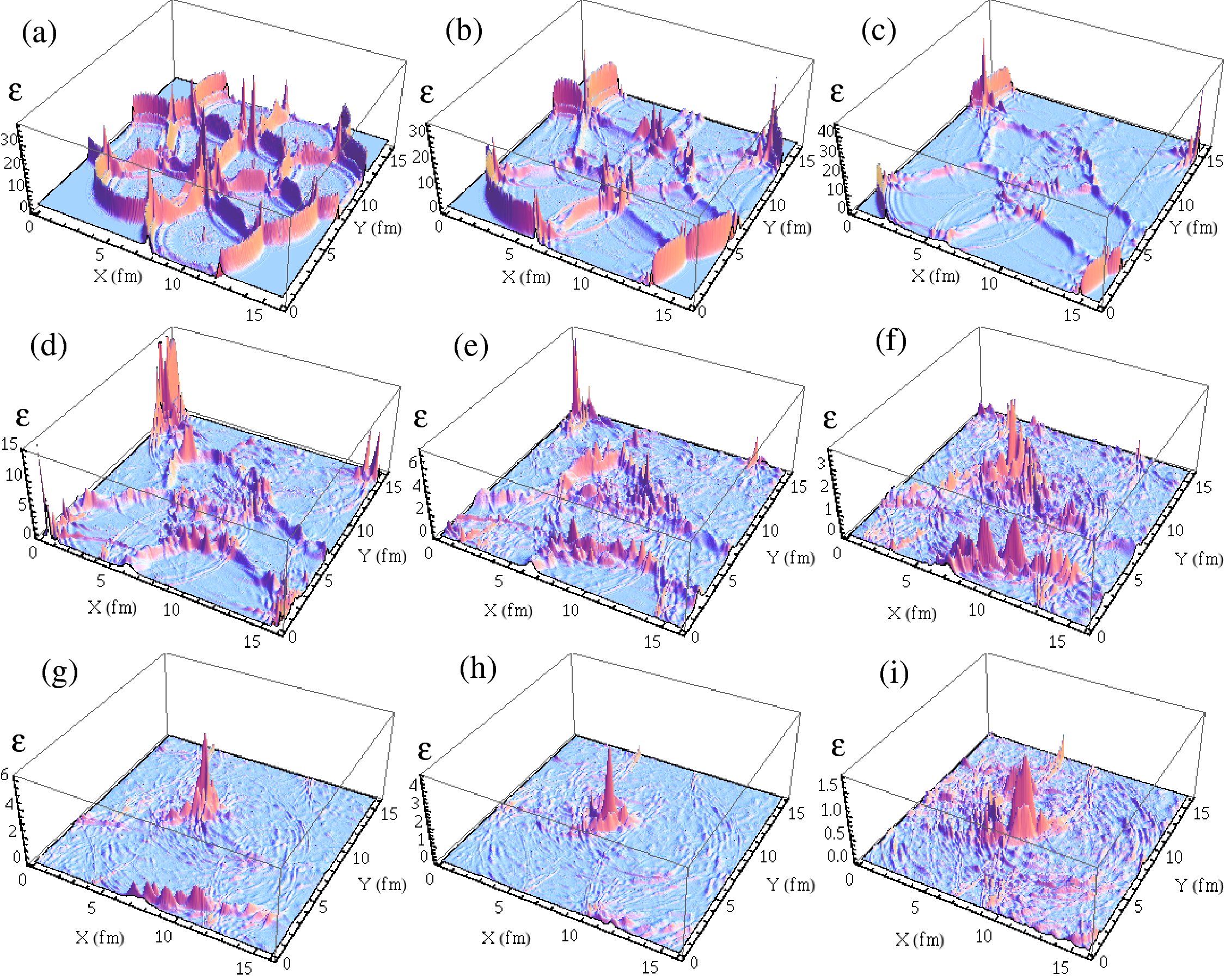
Figure 10:

Surface plots of the local energy density $\varepsilon$ in GeV/fm³. (a) - (i) show plots at $\tau=$ 2.6, 3.5, 4.6, 5.6, 7.0, 8.6, 9.6, 11.2, and 13.2 fm respectively. Formation and subsequent collapse of closed domain wall is clearly seen in plots in (c) through (g). Note that the strong peak in $\varepsilon$ resulting from domain wall collapse (the hot spot) survives in (i) when $T$ = 169 MeV.

Contour plots of $\varepsilon$ are shown in Fig.11. Though closed domain wall can be seen already in Fig.11b (at $\tau=$ 3.5 fm), the domain wall is still attached to outward expanding bubble walls near $X=$ 3 fm, $Y=$ 12 fm which affects the evolution/motion of that portion of the domain wall. Formation of distinct closed wall structure is first visible in Fig.11c at $\tau=$4.6 fm. Subsequent plots clearly show how the domain wall becomes circular and finally collapses away by Fig.11k at $\tau=9.6$ fm. Note the survival of the hot spot even at the stage shown in Fig.11l at $\tau=13.2$ fm when $T=$ 169 MeV.

One can make a rough estimate of the velocity of the closed wall during its collapse from these plots. In Fig.11c, at $\tau=$ 4.6 fm, the $X$ extent of the closed wall is about 8 fm and the $Y$ extent is about 5 fm. The wall collapses away by the stage in Fig.11k at $\tau=$ 9.6 fm. This gives rough velocity of collapse in $X$ direction to be about 0.8 while the velocity in $Y$ direction is about 0.5. Note that here, as well as in Fig.4 for the five bubble case, the estimate of the wall velocity is not affected by the extra dissipation which is introduced only in a very thin strip (consisting of ten lattice points) near the lattice boundary. Formation and collapse of such closed domain walls is important as the resulting hot spot can lead to important experimental signatures. Further, such closed domain wall structures are crucial in the studies of $P_{T}$ enhancement, especially for heavy flavor hadrons as discussed in znb ; apm

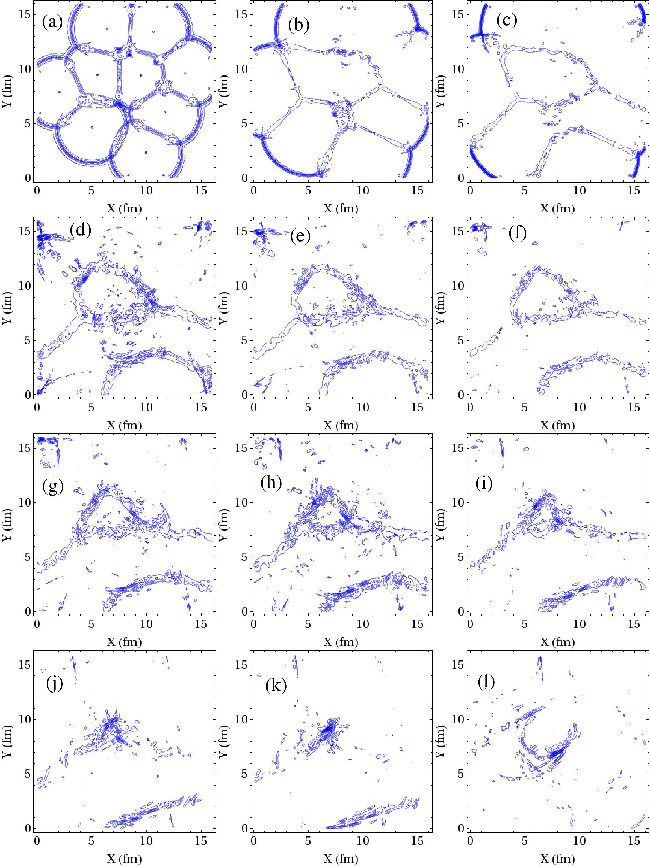
Figure 11:

Contour plots of the local energy density $\varepsilon$ at different stages. Plots in (a) - (l) correspond to $\tau=$ 2.6, 3.5, 4.6, 6.0, 6.6, 7.0, 7.6, 8.0, 8.6, 9.0, 9.6, and 13.2 fm respectively. Formation of distinct closed wall structure is first visible in (c) at $\tau=$4.6 fm. Subsequent plots show the collapse of this domain wall as it becomes more circular. The wall finally collapses away in (k) at $\tau=9.6$ fm. Note that concentration of energy density at the location of domain wall collapse (the hot spot) survives even at the stage shown in (l) at $\tau=13.2$ fm when $T=$ 169 MeV.

Fig.12 shows the evolution of the ratio of the variance of energy density and the average energy density. As for the five bubble case, initial drop and rise are due to heating stage upto $\tau=$ 1 fm and subsequent bubble coalescence and decay of bubble walls. In this case the ratio remain roughly constant upto $\tau\simeq$ 10.5 fm which is the transition stage to the confining phase. This is the stage when the surviving extended domain wall starts decaying. This is also the stage soon after the closed domain wall collapses away. The prominent peak at this stage should be a combined result of both of these effects. The large increase in the variance of energy density at this stage should be detectable from the analysis of particle distributions and should be a clear signal of hot spots resulting from collapse of closed walls and the decay of any surviving domain walls.

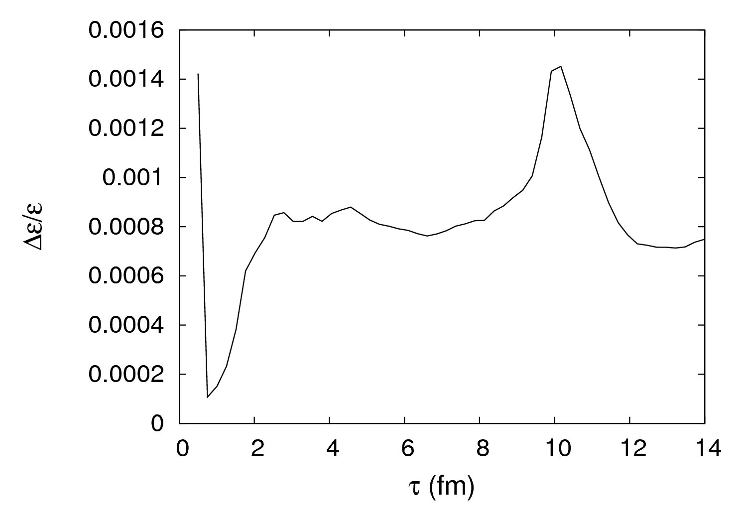
Figure 12:

Plot of the ratio of variance of energy density $\Delta\varepsilon$ and the average energy density $\varepsilon$ as a function of proper time. Energy fluctuations increase during the initial stages when bubbles coalesce and bubble walls decay. After that $\Delta\varepsilon/\varepsilon$ remains roughly constant until the stage when the temperature drops below $T_{c}$ at $\tau\simeq 10.5$ fm. This is also the stage just after the collapse of the closed domain wall. Energy fluctuations sharply increase around this stage. Note the prominent peak at this stage.

VIII Possible experimental signatures of Z(3) walls and strings

The $Z(3)$ wall network and associated strings form during the early confinement-deconfinement phase transition. They undergo evolution in an expanding plasma with decreasing temperature, and eventually melt away when the temperature drops below the deconfinement-confinement phase transition temperature. They may leave their signatures in the distribution of final particles due to large concentration of energy density in extended regions as well as due to non-trivial scatterings of quarks and antiquarks with these objects.

First, we focus on the extended regions of high energy density resulting from the domain walls and strings. This is clearly seen in our simulations and some extended structures/hot spots also survive after the temperature drops below the transition temperature $T_{c}$. Note that even the hot spot resulting from the collapse of closed domain wall in Fig.9,10 will be stretched in the longitudinal direction into an extended linear structure (resulting from the collapse of a cylindrical wall). We know that at RHIC energies, the final freezeout temperature is not too far below the transition temperature $T_{c}$. This means that the energy density concentrated in any extended (sheet like for domain walls and line like for strings/hot spots) regions may not be able to defuse away effectively. Assuming local energy density to directly result in multiplicity of particles coming from that region, an analysis of particle distribution in $P_{T}$ and in rapidity should be able to reflect any such extended regions. In this context, it will be interesting to investigate if the ridge phenomenon seen at RHIC ridge could be a manifestation of an underlying Z(3) domain wall/string structure. Correlation of particle production over large range of rapidity will naturally result from longitudinally extended regions of high energy density (hot spots in the transverse plane). Combined with flow effects it may lead to ridge like structures ridge2 ; ridge . If extended domain wall structure survives in the transverse plane also, this will then extend to sheet like regions in the longitudinal direction. Decay of such a region of high energy density may directly lead to a ridge like structure, without requiring flow effects.

We expect non-trivial signatures resulting from the consideration of interactions of quarks and antiquarks with domain walls. It was shown in an earlier work znb using generic arguments that quarks and antiquarks should have non-zero reflection coefficients when traversing across these domain walls. A collapsing domain wall will then concentrate any excess baryon number enclosed, leading to formation of baryon rich regions. This is just like Witten’s scenario for the early universe wtn (which was applied for the case of RHICE in ref. srfc ). However, for these works it was crucial that the quark-hadron transition be of (strong) first order. As we have emphasized above, in our case formation of Z(3) walls and strings will be a generic feature of any C-D phase transition. Even though we have implemented it in the context of a first order transition via bubble nucleation, these objects will form even if the transition is a cross-over. Thus, concentration of baryons in small regions should be expected to occur in RHICE which should manifest in baryon concentration in small regions of rapidity and $P_{T}$.

Another important aspect of quark/antiquark reflection is that inside a collapsing wall, each reflection increases the momentum of the enclosed particle. When closed domain walls collapse then enclosed quarks/antiquarks may undergo multiple reflections before finally getting out. This leads to a specific pattern of $P_{T}$ enhancement of quarks with heavy flavors showing more prominent effects apm . The modification of $P_{T}$ spectrum of resulting hadrons can be calculated, and the enhancement of heavy flavor hadrons at high $P_{T}$ can be analyzed for the signal for the formation of Z(3) domain walls in these experiments apm . In our simulations extended domain walls also form which show bulk motion with velocities of order 0.5. Quarks/antiquarks reflected from such moving extended walls will lead to anisotropic momentum distribution of emitted particles which may also provide signature of such walls. For collapsing closed domain walls, spherical domain walls were used for estimates in ref. znb and in ref. apm . Our simulation in the present work provides a more realistic distribution of shapes and sizes for the resulting domain wall network. We have estimated the velocity of moving domain walls to range from 0.5 to 0.8 for the situations studied. These velocities are large enough to have important effect on the momentum of quarks/antiquarks undergoing reflection from these walls. One needs to combine the analysis of znb ; apm with the present simulation to get a concrete signature for baryon concentration and heavy flavor hadron $P_{T}$ spectrum modification. We plan to carry this out in a future work. We also plan to study effects of spontaneous violation of CP due to formation of these Z(3) walls in RHICE.

Our results show interesting pattern of the evolution of the fluctuations in the energy density. As seen in Fig.7 and Fig.12, energy density fluctuations show rapid changes during stages of bubble wall coalescence and during collapse/decay of domain walls. Even string-antistring annihilations should be contributing to these fluctuations. Fluctuations near the transition stage may leave direct imprints on particle distributions. It is intriguing to think whether dileptons or direct photons may be sensitive to these fluctuations, which could then give a time history of evolution of such energy density fluctuations during the early stages as well. Even the presence of domain walls and strings during early stages may affect quark-antiquark distributions in those regions which may leave imprints on dileptons/direct photons. An important point to note is that in our model, we expect energy density fluctuations in event averages (representing high energy density regions of domain walls/strings as discussed above), as well as event-by-event fluctuations. These will result due to fluctuation in the number/geometry of domain walls/strings from one event to the other resulting from different distribution of (randomly occurring) Z(3) vacua in the QGP bubbles. Even the number of QGP bubbles, governed by the nucleation probability, will vary from one event to the other contributing to these event-by-event fluctuations.

IX Conclusions

We have carried out numerical simulation of formation of $Z(3)$ interfaces and associated strings at the initial confinement-deconfinement phase transition during the pre-equilibrium stage in relativistic heavy-ion collision experiments. A simple model of quasi-equilibrium system was assumed for this stage with an effective temperature which first rises (with rapid particle production) to a maximum temperature $T_{0}>T_{c}$, and then decreases due to continued plasma expansion.

Using the effective potential for the Polyakov loop expectation value $l(x)$ from ref. psrsk ; psrsk2 we study the dynamics of the (C-D) phase transition in the temperature/time range when the first order transition of this model proceeds via bubble nucleation. As we have emphasized above, though our study is in the context of a first order transition, its results are expected to be valid even when the transition is a cross-over. (Though for non-zero chemical potential the transition may indeed be of first order). The generic nature of our results arises due to the fact that the formation of Z(3) domain walls and associated strings happens due to the a general domain structure resulting after any transition (occurring in a finite time). This is the essential physics of the Kibble mechanism underlying the formation of topological defects in symmetry breaking transitions.

The $Z(3)$ wall network and associated strings formed during this early C-D transition are evolved using field equations in a plasma which is longitudinally expanding, with decreasing temperature. We have neglected here the transverse expansion which is a good approximation for the early stages near the formation stage of these objects, but may not be a good approximation for the later parts of simulations when temperature drops below $T_{c}$ and Z(3) domain walls and strings melt away. We have studied size/shape of resulting closed domain wall as well as extended domain walls and have estimated the velocities of walls to range from 0.5 to 0.8. We also calculate the energy density fluctuations expected due to formation of these objects. Various experimental signals which can indicate the formation of these topologically non-trivial objects in RHICE have been discussed. For example, existence of these objects will result in specific patterns of energy density fluctuations which may leave direct imprints on particle distributions. In our model, we expect energy density fluctuations in event averages (representing high energy density regions of domain walls/strings), as well as event-by-event fluctuations as the number/geometry of domain walls/strings and even the number of QGP bubbles, varies from one event to the other. Extended regions of large energy densities arising from Z(3) walls and associated strings may be manifested in space-time reconstruction of hadron density (using hydrodynamic model). The correlation of particle production over large range of rapidity will be expected from such extended regions. This, combined with the flow effects (for string like regions), or possibly directly (for sheet like extended region) may provide an explanation for the ridge phenomena observed at RHIC ridge . Also, from the reflection of quarks and antiquarks from collapsing domain walls, baryon number enhancement in localized regions (due to concentration of net baryon number) as well as enhancement of heavy flavor hadrons at high $P_{T}$ is expected.

We emphasize again that the presence of $Z(3)$ walls and string may not only provide qualitatively new signatures for the QGP phase in these experiments, it may provide the first (and may be the only possible) laboratory study of such topological objects in a relativistic quantum field theory system.

- (1) U. W. Heinz, Lectures given at 2nd Latin American School of High-Energy Physics, San Miguel Regla, Mexico, 1-14 Jun 2003, published in San Miguel Regla 2003, High-energy physics 165. e-Print: hep-ph/0407360;
- (2) L. D. McLerran and B. Svetitsky, Phys. Rev.D24, 450 (1981); B. Svetitsky, Phys. Rep. 132 , 1 (1986).
- (3) T. Bhattacharya, A. Gocksch, C. K. Altes, and R. D. Pisarski, Nucl. Phys. B 383, 497 (1992); J. Boorstein and D. Kutasov, Phys. Rev. D 51, 7111 (1995).
- (4) A. V. Smilga, Ann. Phys. 234, 1 (1994).
- (5) V.M. Belyaev, Ian I. Kogan, G.W. Semenoff, and N. Weiss, Phys. Lett. B277, 331 (1992).
- (6) C.P. Korthals Altes, hep-th/9402028
- (7) R.D. Pisarski, Phys. Rev. D62, 111501R (2000); ibid, hep-ph/0101168.
- (8) A. Dumitru and R.D. Pisarski, Phys. Lett. B 504, 282 (2001); Phys. Rev. D 66, 096003 (2002); Nucl. Phys. A698, 444 (2002).
- (9) A. Dumitru, D. Roder, and J. Ruppert, Phys. Rev. D70, 074001 (2004).
- (10) B. Layek, A.P. Mishra, A.M. Srivastava, Phys. Rev. D 71, 074015 (2005).
- (11) B. Layek, A.P. Mishra, A.M. Srivastava, and V.K. Tiwari, Phys. Rev. D 73, 103514 (2006).
- (12) ”Z(3) Interfaces, Strings, and their consequences in quark-gluon plasma”, A.P. Mishra, Thesis, Institute of Physics, Bhubaneswar, 2010.
- (13) T.W.B. Kibble, J. Phys. A 9, 1387 (1976); Phys. Rep. 67, 183 (1980);
- (14) W.H. Zurek, Phys. Rep. 276, 177 (1996).
- (15) A. Bazavov, B.A. Berg, and A. Dumitru, Phys. Rev. D78, 034024 (2008).
- (16) M.B. Voloshin, I.Yu. Kobzarev, and L.B. Okun, Yad. Fiz. 20, 1229 (1974) [Sov. J. Nucl. Phys. 20, 644 (1975)]; S. Coleman, Phys. Rev. D15, 2929 (1977).
- (17) O. Scavenius, A. Dumitru and J.T. Lenaghan, Phys. Rev. C66, 034903 (2002).
- (18) G. Boyd, J. Engels, F. Karsch, E. Laermann, C. Legeland, M. Lutgemeier, and B. Petersson, Nucl. Phys. B469, 419 (1996); M. Okamoto et al., Phys. Rev. D60, 094510 (1999).
- (19) S. Chang, C. Hagmann, and P. Sikivie, Phys. Rev. D59, 023505 (1999); M.C. Huang and P. Sikivie, Phys. Rev. D32, 1560 (1985).
- (20) T. Vachaspati and A. Vilenkin, Phys. Rev.D30, 2036 (1984).
- (21) A.M. Srivastava Phys. Rev. D45, R3304 (1992); Phys. Rev. D 46, 1353 (1992); S. Chakravarty A.M. Srivastava Nucl. Phys. B406,795 (1993).
- (22) A.D. Linde Nucl. Phys. B216, 421 (1983).
- (23) J.D. Bjorken, Phys. Rev.D 27, 140 (1983).
- (24) J. S. Langer, Ann. Phys. (N. Y.)54, 258 (1969); J. S. Langer and L. A. Turski, Phys. Rev. A 8, 3230, (1973); L. A. Turski and J. S. Langer, Phys. Rev. A 22, 2189 (1980)
- (25) L. P. Csernai and J. I. Kapusta, Phys. Rev. D 46, 1379 (1992).
- (26) J.I. Kapusta, A.P. Vischer, and R. Venugopalan, Phys. Rev. C 51, 901 (1995)
- (27) P. Danielewicz, Phys. Lett. 146B, 168 (1984)
- (28) T.C. Petersen and J. Randrup, Phys. Rev. C 61, 024906 (2000).
- (29) J. Ignatius, K. Kajantie, and K. Rummukainen, Phys. Rev. Lett. 68, 737 (1992); V. Dixit and M.C. Ogilvie, Phys. Lett. B 269, 353 (1991).
- (30) J. Adams et al. [STAR Collaboration], J. Phys. G 32, L37,(2006) [arXiv:nucl-ex/0509030]; J.Putschke, Talk at Quark Matter 2006 for STAR collaboration), Shanghai, Nov.2006; S. A. Voloshin, Phys. Lett. B 632, 490 (2006)[arXiv:nucl-th/0312065].
- (31) A. Dumitru, F. Gelis, L. McLerran, and R. Venugopalan, Nucl. Phys. A 810, 91 (2008).
- (32) E. Witten, Phys. Rev. D 30, 272 (1984).
- (33) S. Digal, A.M. Srivastava, Phys. Rev. Lett. 80,1841(1998).