PyMorph: Automated Galaxy Structural Parameter Estimation using Python
Abstract
We present a new software pipeline – PyMorph – for automated estimation of structural parameters of galaxies. Both parametric fits through a two dimensional bulge disk decomposition as well as structural parameter measurements like concentration, asymmetry etc. are supported. The pipeline is designed to be easy to use yet flexible; individual software modules can be replaced with ease. A find-and-fit mode is available so that all galaxies in a image can be measured with a simple command. A parallel version of the Pymorph pipeline runs on computer clusters and a Virtual Observatory compatible web enabled interface is under development.
keywords:
galaxies: photometry — galaxies: formation — galaxies: evolution — galaxies: fundamental parameters1 Introduction
In recent years, the morphological analysis of galaxies has provided invaluable information regarding their origin and evolution. This analysis used large galaxy samples drawn from modern astronomical surveys such as the SDSS (York et al. 2000; Abazajian et al. 2009), 2MASS (Skrutskie et al. 2006), GEMS (Rix et al. 2004), COSMOS (Scoville et al. 2007) etc. Since visual estimation of galaxy morphology is most accurate, it is widely used. But given the large numbers of galaxies in astronomical datasets, it is impractical to classify them all using human classifiers (unless a large volunteer base is available, like in the GalaxyZoo project (Lintott et al. 2008)). Besides, different human classifiers may not agree completely on the morphological classification. It is therefore desirable to develop a reliable, objective and automated method for quantitative morphological classification.
It has been known for a long time that the visual morphology of galaxies is well correlated with their physical properties. For example, the colour correlates with the morphology such that late type spirals are bluer, on average, than elliptical galaxies. Similarly, we can make use of the surface brightness profile of galaxies to classify them.
In general, the stellar component of galaxies can be decomposed into a bulge and a disk. While the disk profile is usually an exponential, the bulge is well approximated by the Sérsic function (Sersic 1968). It is found that the bulge-to-total luminosity ratio () of galaxies correlates with the visual morphology where the is the light contained in the bulge component and is the total light of the galaxy. Elliptical galaxies are expected to have , while pure disk galaxies have . In recent years, most researchers prefer to fit a two dimensional representation of the bulge and disk profiles directly to a broad band image of the galaxy (Byun & Freeman 1995; de Jong 1996; Wadadekar, Robbason & Kembhavi 1999; Peng et al. 2002; de Souza, Gadotti, & dos Anjos 2004). This structural decomposition technique is not only useful for quantifying the morphology but is also an excellent tool for studying the formation and evolution of galaxies of different morphological types (eg. Khosroshahi, Wadadekar & Kembhavi 2000; Ravindranath et al. 2001; Simard et al. 2002; MacArthur, Courteau, & Holtzman 2003; Barway et al. 2007, 2009; Vikram et al. 2010). Recent research has shown that the simple Sérsic bulge + exponential disk formulation is not adequate for many galaxies (Laurikainen, Salo & Buta 2005; Gadotti 2008; Peng et al. 2010) and fitting these simple models can lead to wrong estimates of structural parameters. Nevertheless, these simple models, when used appropriately, do give reliable results and are useful indicators of galaxy structure.
Since parametric methods (such as the two dimensional bulge disk decomposition) are generally computational intensive and difficult to apply to small faint galaxies, several non-parametric methods have been developed during the last few years to quantify galaxy morphology. The main motivation for the development of these non-parametric methods is to make classification possible at very high redshifts where the images do not have enough resolution elements and signal-to-noise for visual classification (Abraham et al. 1996; Conselice 2003; Lotz, Primack & Madau 2004). Non-parametric methods are not computationally intensive compared to the parametric methods. However, with non-parametric methods, it is not easy to convert measured quantities to physically meaningful parameters such as bulge or disk luminosity.
In this paper, we describe an automated pipeline software PyMorph to estimate structural parameters of galaxies. We have developed this pipeline by glueing together widely used codes such as SEXTRACTOR (Bertin & Arnouts 1996) and GALFIT (Peng et al. 2002)111Although PyMorph currently uses version 2.5.0 of SEXTRACTOR and version 2.03b of GALFIT , it can easily be modified to use newer versions of these codes. to our own codes for automation and quality control. We have also developed our own implementation of non-parametric methods (Section 2). In Section 3, we explain the operational procedure to obtain structural parameters using GALFIT and SEXTRACTOR. In Section 4, we describe how to setup the pipeline for the parametric and non-parametric methods. In Section 5, we describe the results of the simulations we have done to test the reliability of the pipeline. Finally, we describe a multiprocessor implementation of PyMorph and its performance characteristics (Section 6).
2 Non-parametric methods in PyMorph
We have implemented an automatic procedure for structural decomposition of galaxies using GALFIT supplemented by measurements using non-parametric methods. The algorithms we use to estimate non-parametric quantities are described in Conselice (2003) and Lotz et al. (2004). For completeness, we summarise the main features of these algorithms. For the calculation of all non-parametric quantities we use the sky value and center as determined by SEXTRACTOR , whereever required. Also, we use the SEXTRACTOR source catalog to identify and mask neighbour objects.
2.1 Concentration index ()
Concentration is defined as the ratio of the radius of the galaxy which contains 80% of the total light () to the radius of the galaxy which contains 20% of the total light (). ie.,
| (1) |
Here, the total light of the galaxy is taken to be the light within 1.5 times of the Petrosian radius (hereafter extraction radius, ) where is the radius of the galaxy at which the Petrosian parameter takes a value of 0.2. The Petrosian parameter is defined as follows:
| (2) |
where is the average light at the radius and is the average light inside . Near the center of the galaxy, where the light profile changes rapidly, we need to oversample the pixels to obtain an accurate measurement. We achieve this by subpixelisation inside the central 7 pixels (radius) of the galaxy by a factor of ten.
2.2 Asymmetry ()
We calculate asymmetry using the algorithm devised by Conselice (2003). The steps are: we rotate the galaxy through 180 degrees about its center which is taken to be the centroid (first image moment) of the galaxy pixels. We use bilinear interpolation to obtain the rotated image. In the next step, we substract the rotated image from the original image of the galaxy. From the residual image we estimate the total residual flux inside the extraction radius. This is then normalised by the total flux of the galaxy. This step can be represented as follows:
| (3) |
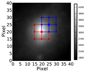
where and are original image and the rotated image respectively and the summation is over all valid pixels excluding the pixels contaminated by light from neighbouring objects, inside the radius . In the next step, we identify possible biases in the measured asymmetry value and correct for them. The first bias to the estimated asymmetry value is due to the uncertainty in the estimated centroid of the galaxy. For example, a perfectly symmetric galaxy can give non-negligible asymmetry value if we cannot determine the centroid of the galaxy exactly. To correct for this bias we minimise the asymmetry with respect to the center. To do that, we create a square grid of nine points which includes the initial centroid of the galaxy. The bin width of the grid of points is a fixed fraction of the half light radius of the galaxy (). We find asymmetry of the galaxy about all these nine points, and assign the point corresponding to the minimum asymmetry as the new centroid of the galaxy. We then generate a new grid of points described as above, find the asymmetry of the galaxy about this newly created grid of points and again determine the minimum asymmetry. This process continues until we reach a stable point where the asymmetry is minimum about that point compared to the estimated asymmetry of the galaxy about the neighbouring points. This process is illustrated in Figure 1 (Conselice 2003).
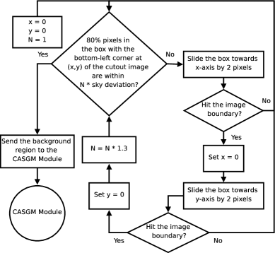
The second bias is introduced by the gradient of the sky near the object. To compensate for this, we estimate asymmetry of the sky and substract it from the object asymmetry. To get the background asymmetry we find an empty region near the object, which should represent the real sky at the object position and therefore, cannot be far from the object. On the other hand, it is difficult to get an empty sky region very near to the object. This forces us to use an optimum distance from the object center to search for the sky region (This distance is same as the dimension of cutout of the object. We explain this in section 3.2). We mask all the objects in the cutout and estimate the sky standard deviation (). Then, to identify a region of blank sky within the cutout, we put a square region at the bottom left corner of the cutout with a size X. We find that pixels is optimal to get background asymmetry. Inside the square region identified as possible blank sky, we check how many pixels are within . Initially, we take N = 1. If we cannot find at least 80% of the pixels within this range we slide the square by 2 pixels along the x axis and repeat the procedure. If we do not find a suitable blank sky region, this process continues until we hit the image boundary. Then we slide the blank sky search square along the y axis. If we fail to find a region after searching the whole image, we assume that the sky has a large gradient. Therefore we increase N by 1.3 times and search sky region inside as we did earlier. This simple approach may fail when we have a highly crowded field. In such situations, PyMorph notifies the user of the problem by setting the proper flags. This process is summarised in Figure 2.
After we find an empty sky region we mask all pixels with counts outside and find the asymmetry of that region and minimize it in the same way as we did in the case of the object. Finally, we subtract the minimised background asymmetry from the minimised object asymmetry to get the ’true’ asymmetry which can be represented as:
| (4) |
where is the composite asymmetry of both object and sky, is the asymmetry of the sky and is the true asymmetry (Conselice 2003).
2.3 Clumpiness ()
The clumpiness is a quantitative measure of clumpy regions in the galaxy. These are associated with star forming regions and thus clumpiness of spiral galaxies is larger, on average, than that of elliptical galaxies. To find we convolve the galaxy image with a boxcar function of width where is the Petrosian radius of the galaxy. This smoothed image is then subtracted from the original image and the residual is summed within the extraction radius. During this process, we mask the central part of the galaxy as those regions are unresolved. The output of this process is the sum of the clumpiness of the object and background. To get the clumpiness of the object alone, we find the background clumpiness and substract it from the composite value. The background region used for this purpose is same as that used for the asymmetry calculation. The whole process can be summarised in the following equation:
| (5) |
where is the original image, is the smoothed image and the summation is over all the positive pixels of residual image with the annular region of width . is the clumpiness of the background region (Conselice 2003).
2.4 Gini coefficient ()
It has been found that the Gini coefficient is a powerful way to describe the morphology of a galaxy (Lotz et al. 2004). This coefficient can be regarded as a generalized concentration parameter. If all the light in the galaxy belongs to a single pixel, the Gini coefficient takes a value of 1. On the other hand, if the total light distributes uniformly among all the pixels belongs to the galaxy, then the Gini coefficient will be 0. On average, an elliptical galaxy has a larger Gini coefficient than a disk galaxy.
To get we need to find the pixels in the image which belong to the galaxy, i.e. obtain the segmentation map of the galaxy. This is important as will be underestimated if we include sky pixels and will be overestimated if we miss the outer pixels of the galaxy. To determine which pixels belong to a galaxy, we convolve the galaxy image with a boxcar filter of size . This process will increase the signal to noise ratio in the outer parts of the galaxy. Then we measure the surface brightness at . We assign all the pixels in image with to the galaxy where is the standard deviation of the sky. The upper limit ensures that no cosmic rays or spurious pixels are included in the segmentation map. Then the pixels belonging to the segmentation map are sorted according to their photon count and is calculated using the equation:
| (6) |
where is the photon count in the pixel which belongs to the segmentation map, is the mean of all the pixel values and is the total number of pixels (Lotz et al. 2004).
2.5 Second order moment of the brightest pixels ()
This quantity gives an idea of how the brightest pixels are distributed over the galaxy segmentation map. For elliptical galaxies, the brightest pixels are concentrated near the center of the galaxy. Therefore, the parameter will be smaller for ellipticals compared to spiral galaxies where we observe large number of star forming regions distributed all over the galaxy. To compute we use the segmentation map generated to estimate the Gini coefficient. We start by computing the flux weighted second order moment of the galaxy as
| (7) |
where , , are the flux value and x and y coordinates of the pixel in the segmentation map and and are the initial center of the galaxy. We then minimize with respect to the center of the galaxy as the initial value of the center is the centroid of the galaxy. In the next step we sort the pixels according to their flux value and find the moment of the 20% brightest pixels of the galaxy using the equation
| (8) |
where the summation continues until it satisfies where is the pixel in the sorted array of the segmentation map and is the total light of galaxy (Lotz et al. 2004). It can be seen that when calculating the pixels are weighted by which results in a large value for galaxies with many star forming regions distributed away from its center. Therefore, will be smaller for passbands which map the underlying old stellar distribution (e.g. near IR) than those which map the young stellar population (e.g. near UV).
3 Estimating structural parameters of galaxies
Many well tested codes are available to perform 2D decomposition. These include FITGAL (Wadadekar et al. 1999), GIM2D (Simard 1998), GALFIT (Peng et al. 2002), BUDDA (de Souza et al. 2004) etc. Although the basic working principles of these codes are the same, they implement different minimisation algorithms. FITGAL uses the Davidon-Powell-Fletcher minimisation algorithms as implemented in the minuit code developed at CERN (James 1994) while GIM2D minimisation uses the Metropolis Algorithm. Marquardt-Levenberg minimization drives GALFIT and BUDDA uses a multidimensional downhill simplex method (Press et al. 1992). Because of the complexity of the parameter space it is very important to carefully setup the minimisation so that these codes find the global minimum, as far as possible. In PyMorph, we have chosen to use GALFIT for 2D decomposition because of its simplicity and faster convergence. However, the pipeline is designed in a modular way so that the minimisation engine can be easily changed at a future date, if required.
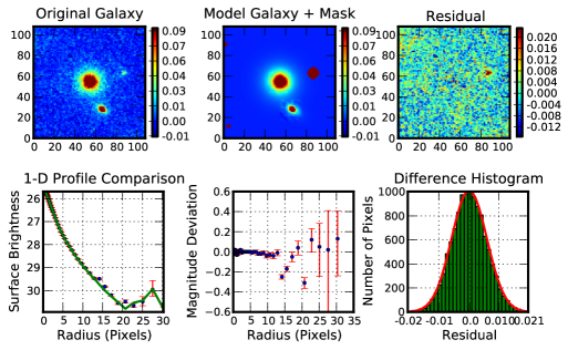
The main preparatory steps before running GALFIT are: 1. Detect objects in the input image and obtain their photometric parameters using SEXTRACTOR ; (again, the pipeline can be easily modified to use another source extraction software) 2. Create a cutout of the main object; 3. Create an appropriate mask image to reject neighbour objects and spurious pixels; 4. Create a configuration file for GALFIT. Besides 2D fitting, PyMorph also performs the following tasks for every galaxy that it fits: 1. Generates a one dimensional profile of input and best fit model galaxy using the IRAF/STSDAS ellipse task to facilitate visual checks for obvious fitting errors; 2. Converts all the fitted parameters to physical parameters using the user specified cosmology and the galaxy redshift (if available) 3. Creates outputs in several formats which includes CSV and html and stores results in a mysql database; 4. Creates diagnostic plots in png format (see example in Figure 3).
3.1 Object detection and photometry
This is the initial stage of PyMorph. We use SEXTRACTOR to detect objects in the input image and perform photometry on them. The input image may either be a large frame or a cutout of the galaxy of interest. If the image is a large frame, the astronomer may be interested only in a few specific objects in the frame or may want to generate parameters for all galaxies in the frame that satisfy some selection criteria. In either case, before proceeding, a catalog with the exact location and magnitude of the objects of interest is needed. To obtain such a catalogue, PyMorph runs SEXTRACTOR on the input image to generate a SEXTRACTOR photometric catalogue. The SEXTRACTOR output parameters used by PyMorph are X_IMAGE, Y_IMAGE, ALPHA_SKY, DELTA_SKY, FLUX_RADIUS, THETA_IMAGE, A_IMAGE, ELONGATION, ISO0, BACKGROUND, CLASS_STAR and MAG_AUTO. X_IMAGE and Y_IMAGE are the x and y coordinates respectively of the centroid of the object in pixel units. ALPHA_SKY, DELTA_SKY are the RA and DEC of the object. FLUX_RADIUS is the half light radius. THETA_IMAGE, A_IMAGE, ELONGATION represent the position angle, the semi-major axis length (a) and ratio of the semi-major to semi-minor axis length of the object. SEXTRACTOR divides the detected objects into eight isophotal levels above the ANALYSIS_THRESH. ISO0 represents the area of the object above the ANALYSIS_THRESH in units of pixel2. MAG_AUTO, BACKGROUND and CLASS_STAR are the magnitude, background value at the object position and the stellarity parameter of the object. The user can choose the SEXTRACTOR local or global background. CLASS_STAR for a star and for a galaxy.
3.2 Position match and object cutout generation
After the SEXTRACTOR catalogue is created, the program compares the user given input catalogue of objects (which lists the galaxies of interest) with the SEXTRACTOR catalogue. For each object in the input catalogue, PyMorph finds the corresponding entry in the SEXTRACTOR catalogue either by matching the RA and DEC coordinates or by matching pixel coordinates. The matching radius can be set by the user, either in units of pixels or in arcsec. For every successful match between the input catalog and the SEXTRACTOR catalogue, PyMorph reads all the required SEXTRACTOR photometric parameters of that object for further use.
The next step is to create a cutout image of the object to feed to GALFIT. The size of the cutout image should be such that it contains enough sky pixels without becoming very large in size. The first criterion is highly desirable as insufficient number of sky pixels may cause incorrect background estimation by GALFIT. This will seriously affect the estimation of Sérsic index of the bulge. On the other hand, including a large sky region in the cutout will increase computational resource requirements. We use the SEXTRACTOR FLUX_RADIUS (), ELONGATION () and THETA_IMAGE () parameters to find the optimum size of the cutout as follows:
| (9) |
where and are the dimension of the cutout centered on the galaxy center and is a user specified parameter. Through trial and error, we found that gives optimum size for the cutout image. Using the size and the centroid parameters of the object, we cut the portion of image and the corresponding weight image (if available).
3.3 Create mask image
An advantage of GALFIT is that it allows us to simultaneously fit any number of objects. But it is not advisable to fit many objects simultaneously as that increases the number of free parameters. In such situations, the fit may converge to a local minimum. Therefore, we should simultaneously fit for a neighbouring object only if it is large and/or bright enough to significantly contaminate the main object. To decide whether a neighbouring object should be included in the simultaneous fitting, we use the A_IMAGE, ISO0 parameters of each object. We compare the parameters of all neighbouring objects in the SEXTRACTOR catalogue with those of the object of interest. We check whether the objects overlap with the main object by comparing their scaled semi-major axis (the scale is user specified). The scale determines the distance to the closest neighbour to be fitted simultaneously with the object. For e.g., let us say that the distance between the centers of the object of interest and its neighbour is 100 pixels, the semi-major axis of the object of is 60 pixels and that of the neighbour is 30 pixels. Then, even if the galaxies have circular shape they will not overlap (because ) and the neighbour will therefore be masked. If the user requires that such neighbours be fitted simultaneously, the scale parameter can be tweaked. If the scale parameter is set to 2, then and now the neighbour will be fitted simultaneously with the object. If the program finds overlapping neighbours, it also checks whether the area of the neighbour is larger than a user specified fraction of the main object. If the area (ISO0) of the neighbour is higher than a threshold fraction of the area of the object of interest, then it will be fitted simultaneously. If the neighbour’s area is below the threshold fraction, then that neighbour will be masked irrespective of its distance from the object. Therefore the condition for simultaneous fitting is as follows:
| (10) |
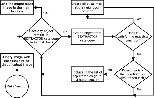
where is the distance between object and neighbour, and , are the A_IMAGE parameters and and are the ISO0 parameters of object and neighbour respectively. is a user specified parameter which decides the threshold fraction of overlap between object and neighbour. The value of decides the smallest object which is to be included in the simultaneous fit with the object of interest. We found the control parameters and give good results. Neighbours which do not satisfy the simultaneous fit criterion in Eqn 10 are masked out. To do this, PyMorph creates an elliptical mask at the position of the object. This mask has the same ellipticity as that of the neighbour but its semi-major axis is scaled by an amount which is also to be specified by the user. i.e., the semi-major axis of the mask becomes . This process continues for all the objects in the SEXTRACTOR catalogue and finally we have a mask image that is the union of masks for all the contaminating objects. The block diagram describing this process is shown in Figure 4.
This masking technique works only if SExtractor detects the neighbouring object, in the first place. Since that process depends on the DETECT_THRESH and DETECT_MINAREA parameters the user chooses, it is possible that some spurious pixels bright enough to affect the fit may be left undetected by SExtractor. So, we use the following simple technique to mask such pixels. From the center of the main object, we make elliptical annuli with increasing radii. In the inner aperture we find the maximum value of the galaxy. We assume a smooth light distribution for the galaxy which decreases with distance from the center. This implies that the largest value in the central elliptical aperture is the maximum value the object can have. So, we mask all the other pixels outside the inner aperture with value greater than this maximum value. Now we go to the next pair of annuli and find the maximum and mask other pixels outside this aperture which have value larger than the maximum of this aperture. This procedure continues till the aperture radius hits the image limit. Using this technique we are likely to mask small regions with a high flux e.g. knots of star-forming regions in spiral arms. However, since we are attempting to determine global parameters for the bulge and disk of the galaxies, masking out local fluctuations over the underlying bulge and disk will likely only improve the parameter estimation. However, if desired, one can switch off this masking technique setting the ’mask-norm’ option. In that case, only the neighbour objects will be masked. Now, almost all the spurious pixels which may be part of undetected objects should be masked correctly. We combine this mask image with the mask image made using the SEXTRACTOR catalogue to get the final mask.
3.4 Create configuration file for GALFIT
GALFIT configuration can be done either through a text file or through the command line. Pymorph creates an input configuration file for each object in the user given catalogue to feed GALFIT. This file specifies the filenames of the input image, the weight image and the point spread function image. The other entries include initial values of the parameters of the components used in the fitting. For two dimensional decomposition, a galaxy is usually assumed to have, at least, a bulge and a disk component. The bulge is modeled by a Sérsic function of the form
| (11) |
where is the intensity of the bulge at radius , is the intensity of the bulge at radius , is the half light radius and is the Sérsic index of the bulge. is a quantity which depends on . Similarly, the disk part is usually modeled using the exponential form
| (12) |
where is the disk intensity at the centre and is the disk scale length. The surface brightness profile of the galaxy is modeled as a linear combination of these two functions.
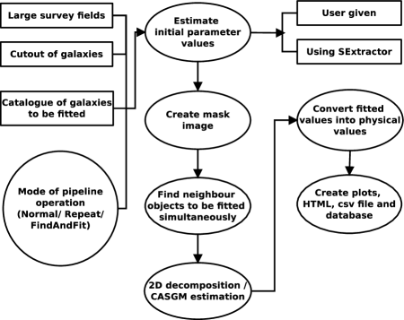
There are more than a dozen parameters to be fitted during the decomposition of a galaxy. These include the centers of bulge and disk components and their total magnitudes, scale radii, axis ratio and position angles. Sérsic index of the bulge is another parameter involved in the fitting. GALFIT offers two additional parameters which model the boxiness/diskiness of the bulge and disk. We have not used these parameters in our fits. Apart from the parameters involved in the photometric components of the galaxy, one other important parameter is the sky. There is an option in GALFIT to fit sky with gradient in x and y directions of the image. To increase our chances of finding the global minimum from GALFIT , we need to set the appropriate initial values for the fit parameters. We use SEXTRACTOR MAG_AUTO and FLUX_RADIUS parameters of the galaxy as the initial values for the total magnitudes and scale radii of both bulge and disk. The initial values of the axis ratios of both bulge and disk are set from the SEXTRACTOR ELONGATION parameter and position angle is calculated from THETA_IMAGE. We always set the initial value for the Sérsic index to 4. The sky parameter is set to the SEXTRACTOR value. We found that SEXTRACTOR slightly overestimates the background value which can result in incorrect estimation of bulge parameters. This issue will be discussed in Section 5.1. The working of PyMorph is summarised as a block diagram in Figure 5.
4 Setting up PyMorph
PyMorph is written entirely in the Python programming language. Python is a modern, high level programming language with many features that encourage readable and reusable code. Several current astronomical data analysis systems have been made accesible through Python (e.g. Pyraf for IRAF and CASA.py for AIPS++). Python will play a major role in many new software initiatives in astronomy.
Besides the standard python modules, additional modules required by PyMorph are numpy, matplotlib and pyfits. Numpy is used for arithmetic manipulations on the image array and matplotlib is used to generate output plots. Pyfits is a python module to read and write fits images. As we have already mentioned, SEXTRACTOR and GALFIT currently serve PyMorph as the detection and fitting programs. Since all the required processing for 2D decomposition is pipelined, the user needs to initialize the code correctly so that it completes without needing further intervention. All the required input parameters can be set through an input configuration file. Some parameters can be give to PyMorph via command line as well. An example input configuration file for PyMorph is shown in Figure 6.
(A) ###----Specify the input images and Catalogues----### imagefile = ’j8f643-1-1_drz_sci.fits’ whtfile = ’j8f643-1-1_drz_rms.fits’ #The weight image. sex_cata = ’j8f643_sex.cat’ #The sextractor catalogue clus_cata = ’cl1216-1201.cat.old’ #The input catalogue of galaxies (B) ###----Specify the output images and catalogues----### out_cata = ’cl1216-1201_out.cat’ #catalogue of galaxies in the field rootname = ’j8f643’ (C) ###----Point spread function list----### psflist = ’@psflist.list’ #List of psf stars mag_zero = 25.256 #magnitude zero point (D) ###----Conditions for Masking----### mask_reg = 2.0 thresh_area = 0.2 threshold = 3.0 (E) ###---Size of the cut out and search conditions---### ###---size = [resize?, varsize?, fracrad, square?, fixsize]---### size = [0, 1, 6, 1, 120] #size of the stamp image searchrad = ’0.3arc’ #The search radius (F) ###----Parameters for calculating the physical parameters of galaxy----### pixelscale = 0.045 #Pixel scale (arcsec/pixel) H0 = 71 #Hubble parameter WM = 0.27 #Omega matter WV = 0.73 #Omega Lambda (G) ###----Parameters to be set for calculating the CASGM----### back_extraction_radius = 15.0 angle = 180.0 (H) ###----Fitting modes----### repeat = False #Repeat the pipeline manually galcut = False #True if user provides cutouts decompose = True #Find structural parameters cas = True #Find CASGM parameters findandfit = 0 #Run for all objects which satisfies user defined criteria crashhandler = 0 (I) ###---Galfit Controls---### components = [’bulge’, ’disk’] #The components to be fitted to the object ###---fixing = [bulge_center, disk_center, sky] fitting = [1, 1, 0] # = 0, Fix params at SExtractor value (J) ###----Set the SExtractor and GALFIT path here----### GALFIT_PATH = ’/home/vinu/software/galfit/modified/galfit’ SEX_PATH = ’/home/vinu/software/sextractor-2.5.0/sex/bin/sex’ PYMORPH_PATH = ’/home/vinu/ncra/vinucodes/serial_pipeline/trunk/pymorph’ (K) ###----The following conditions are used to classify fit as good/bad----### chi2sq = 1.9 #< chi2sq center_deviation = 3.0 #< abs(center - fitted center) (L) ###----Database Informations----### database = ’cluster’ table = ’clusterfitresults’ usr = ’vinu’ pword = ’cluster’ dbparams = [’Cluster:cl1216-1201’, ’ObsID:1:int’]
There are 12 blocks in the configuration file. Most of the parameters in blocks A and B are self-explanatory. The parameter psflist corresponds to a file containing the list of suitable PSF images. These may be stellar images from the input frame (typically unsaturated, isolated bright stars) which the user feels are accurate representations of the PSF. It is known that in large frames the PSF may vary spatially. Therefore the general principle is to use the nearest star to the object as the PSF. If the names of these stellar images follow the convention psf_RaDec.fits, eg. psf_1216382-1200443.fits, then PyMorph will automatically find the nearest PSF to the object from psflist and use it for fitting, otherwise it assumes that there is a one to one correspondence between the list of PSFs and galaxies to be fitted. The thresh_area and threshold parameters in block D correspond to and respectively in Eqn. 10. mask_reg () determines how much area of the neighbour should be masked.
The size keyword is a list of five parameters which control the size of the cutout image. The first one in the list is a flag that tells the program to create a cutout of the object. This is needed sometimes when the user already has a cutout of the objects. In those situations, this parameter should be unset. Using the second entry in the list, the user can set the size of the cutout of all the objects fixed at a particular value irrespective of the real size of the object. If the user wants to create cutout of objects scaled by their angular size, the size of the cutout will be determined by the third parameter in the list. This is the quantity involved in Eqn. 9. The fourth quantity determines shape of the cutout. If the user sets the parameter, then the cutout will have a square shape with size equal to the maximum of and which is given by the Eqn. 9. Otherwise the cutout will have rectangular shape of size and . The final entry in the list is used if the user does not set the second entry. e.g. an entry size = [1, 1, 6, 1, 120] tells the program to create a cutout, measure size from the objects, that the size should be six times larger than the half light radius of the objects and to make a cutout of square shape. On the other hand, if the user sets the size keyword as [1, 0, 6, 1, 120], then the program will create a cutout of size irrespective of the size of the galaxy.
The parameter searchrad is the search radius used to match the input catalogue with the SEXTRACTOR catalogue. The comparison can either be in pixels or in arcsec. Therefore if the user set searchrad = ’0.3arc’ then the program matches objects within 0.3 arcsec. On the other hand, the entry searchrad = ’5pix’ matches objects within 5 pixels. The cosmological parameters in the block F will be used to convert the fitted parameters to physical units. The G block parameters will be used for the calculation of asymmetry of objects. Through back_extraction_radius parameter the user can set the size of the background region which will be used to find the asymmetry of the background. The parameters in block H determine the different modes of PyMorph behaviour. galcut should be set if the user wants to supply cutouts of galaxies. decompose and cas should be set to get parametric and non-parametric results respectively, from PyMorph. The findandfit is implemented in order to get the structural parameters of all the objects in large frame(s) which satisfies some user defined criteria. For example, this mode can be used if the user wants to generate the structural parameters for all objects in a frame between magnitudes and . If crashhandler is set then the program automatically reruns GALFIT for some obvious fitting errors. In the presence of a bright neighbour or dust lanes in the galaxy, the best fit center of either bulge or disk can be significantly different from the optical centroid of the galaxy. Pymorph tracks errors at all the stages of the pipeline and saves those errors as flags. Therefore it is possible to identify the stages of the pipeline that have failed, in some way. The obvious fitting errors include incorrect centers, ie. the fitted center of the component is very far from the visible center of the galaxy, or some parameters have hit the limit of their allowed range. After a fitting process finishes, pymorph checks for these errors. If the program finds an incorrect center, the galaxy is refit with tight constraints on the range of center. If the program finds a parameter that hits the limit, then it increases the fitting range and carries out a refit, which may give a better result. If the refit also fails, the galaxy is flagged as a poor fit (indicated in the FIT parameter in the output catalogue). Finally, the repeat mode is implemented to rerun PyMorph semi-automatically. It is possible that GALFIT converges to a local minimum for a few galaxies. Then the user can edit the corresponding GALFIT configuration file, mask etc. to rerun GALFIT again, if the pipeline is set to run in repeat mode. Pymorph generates all the necessary intermediate files to do decomposition which includes the mask, GALFIT configuration files etc. and saves them to disk. If the user finds that GALFIT failed to converge to a global minimum because of improper initial values of the parameters or a poor mask image, then the user can manually edit the mask image or slightly alter the GALFIT initial values. After this, the user can set the repeat mode and run pymorph. In that case, pymorph uses the existing intermediate files to run GALFIT without generating them anew.
The I block parameters controls GALFIT. Through components keyword the user can set the number of photometric components of galaxies for fitting. If components = [’bulge’, ’disk’], then a Sérsic and an exponential function will be fitted to the galaxy’s surface brightness. Through fitting the user can fix/free the centers of the fitting functions and sky. For example, fitting = [1, 1, 0] tells the program to set the centers of the bulge and disk as free parameters and fix sky at the initial value during fitting. The program reads the location of SEXTRACTOR , GALFIT and PyMorph from the J block. The K block parameters will be used to determine whether a given fit is acceptable or not. This includes the simple reduced (chisq) and center_deviation. center_deviation is a measure of the difference between the initial and fitted centers of the components in pixel units. If this difference is greater than center_deviation, then the corresponding fit will be considered as bad. This will be refitted with tight constraints on the centers provided the user has set crashhandler parameters in the H block. The final L block deals with the output database. If the program finds a mysql database server then these parameters become active. All other parameters in this block are self explanatory other than dbparams. Through dbparams the user can create additional columns in the database table and set their values. For example, dbparams = [’Cluster:cl1216-1201’, ’ObsID:1:int’] will create two additional columns Cluster and ObsID in the current database table. The functions of different blocks in the PyMorph configuration file are summarised in Table 1
| Block | Function |
|---|---|
| A | Input images and catalogues |
| B | Output files |
| C | PSF file |
| D | Masking conditions |
| E | Cutout size |
| F | Cosmology |
| G | CASGM parameter measurement |
| H | Fitting Modes |
| I | GALFIT controls |
| J | Set path to software |
| K | Classification criteria |
| L | Database information |
5 Testing the robustness of PyMorph
5.1 Caveats of pipeline use
Before we describe the tests we carried out to examine the robustness of the Pymorph pipeline we would like to caution the user against using it blindly without accounting for its limitations. Specifically:
-
1.
A linear combination of bulge and disk is inadequate to model galaxy structures such as a nuclear point source, bars, rings etc., whenever they are sufficiently strong. Adding analytic models for these components greatly increases the free parameters in the minimisation making it more likely to converge to an incorrect local minimum. Automated procedures that attempt to fit all these components are unlikely to give reliable results. We have therefore deliberately not added the ability to fit additional components to Pymorph. GALFIT does provide for modelling these features, but one needs to run it carefully on individual galaxies. In the rest frame near-infrared, components like star forming knots are quite weak. In addition, for distant galaxies, these small scale features will be blended with the large scale bulge and disk. In such cases, a linear combination of bulge and disk will likely be a robust model of the galaxy structure, although its physical interpretation is more complicated.
-
2.
Certain minimisation algorithms are more prone to converge to local minima (e.g. Levenberg-Marquardt used by GALFIT ) than others (e.g. Metropolis algorithm used by GIM2D). In practice, Häussler et al. (2007) have shown that GALFIT works better than GIM2D in many situations. Users need to be aware of the capabilities and limitations of the algorithm and specific implementation being used.
-
3.
Häussler et al. (2007) have pointed out that the SEXTRACTOR sky determination tends to overestimate the background. Incorrect background determination can affect parameter estimation, especially those of the bulge.
-
4.
If one is fitting a pure disk galaxy, it often gets incorrectly fit by a Sérsic function with . This results in , which is clearly incorrect.
In order to assist the user in determining whether a particular galaxy has been correctly fit, Pymorph provides a diagnostic plot (see sample in Fig. 3). We recommend the following procedure to test for the quality of the fit, which users may adapt to their requirements.
-
1.
Check whether the FIT parameter in the output catalogue is unset. If it is unset it means that the reduced is larger than that the user specified in the config.py or the fitted center of at least one component is incorrect.
-
2.
Check for large residuals near the centre of the residual image in the diagnostic plot, which may be caused by a wrong PSF.
-
3.
Check whether the difference histogram is centered at zero and well matched to the best fit Gaussian. If not, the residual image is not purely composed of noise.
-
4.
Check whether the one dimensional profiles of original galaxy and the model galaxy match.
Through experience, the user will be able to rapidly identify problematic fits. Some of the quality checks above can be automated via scripts that use the information contained in the ASCII output files (result.csv) produced by Pymorph. Galaxies that are poorly fit may be handled using PyMorph in repeat mode (see Section 4).
5.2 Compare extracted CASGM parameters with published values
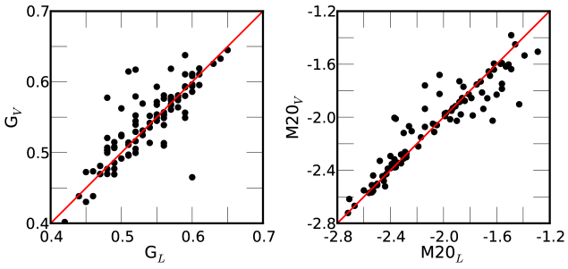
We have used a well studied sample of nearby galaxies (Frei et al. 1996) with publicly available data to test the robustness of the CASGM parameters. We compare our estimated values with published values for these galaxies by Conselice (2003) and Lotz et al. (2004). This gives an idea of the robustness of our automated procedure. Figures 7 and 8 show the result of this comparison. We calculated the dispersion between our values and the published values. We found that the average deviation for concentration, asymmetry and clumpiness from that of Conselice (2003) are -0.11 0.14, 0.0 0.036, 0.06 0.09 respectively. The average dispersion of our estimated values for Gini coefficient and second order moment with that of Lotz et al. (2004) are 0.0 0.035 and 0.0 0.16. It will be interesting to compare the CAS values of Conselice (2003) with those Lotz et al. (2004) to show that similar dispersion was seen in previous comparisons. The dispersion between the CAS parameters reported in those papers are 0.08 0.16, -0.04 0.0445 and 0.01 0.08 for , and respectively.
The small systematic offset of our concentration measurement from that of Conselice (2003) (see left panel of Figure 7 is due to the slight error in measuring the background value. This error will propogate to the measurement of and values. This effect is stronger in the case of galaxies with high concentration as they will have smaller and the slight uncertainty in leads to some variation in concentration index. It should be noted that this offset, though real, is small and within the error in many cases.

5.3 Simulating two dimensional galaxy light profiles
To test the robustness of the structural parameters given by PyMorph we have run the code on simulated galaxy light profiles. In this section, we describe the simulation and then discuss the results. We simulate surface brightness profiles of galaxies as a linear combination of a Sérsic and exponential functions. The steps involved in the simulation are the following:
1. Set the values of the parameters involved in the Sérsic and exponential functions. The range of these parameters used for simulation are 18 25, 1 kpc 6 kpc, 1 kpc 10 kpc, 0.4 0.9, 0.2 0.9 where , , are the apparent magnitude, scale radius and axis ratio of bulge component of the galaxy and , are the apparent magnitude, scale radius and axis ratio of the disk component. The range of Sérsic index used is . These parameters are distributed uniformly along their respective ranges.
2. The Sérsic function is steeper towards the center for large values of Sérsic index. Therefore, it is important to treat this cusp differently to generate exact surface brightness in the central region. We do this by oversampling the Sérsic function at the center region. We oversample the central pixels by a factor of 10. At the central pixel, we oversample the function 30 times while conserving the flux. For exponential function, the oversampling is done with a factor of 10.
3. We simulated 1000 objects as described in the previous step and inserted them into a array. The position of these galaxy profiles in the large array are distributed randomly. This process is intended to simulate the original observation.
4. We then convolved the model image by the PSF. We have extracted a stellar image from an ACS observation for this purpose.
5. To simulate noise, we have generated a background image which has a typical standard deviation of the original observations of HST ACS/WFPC2. The background values are distributed according to the Poisson distribution. Along with the background image we propagate the statistical error of the object counts determined from model image to create the noise image.
6. The model image and the background images are added to get the final simulated images and these images are used for further analysis.
5.4 Regression results for simulated galaxies
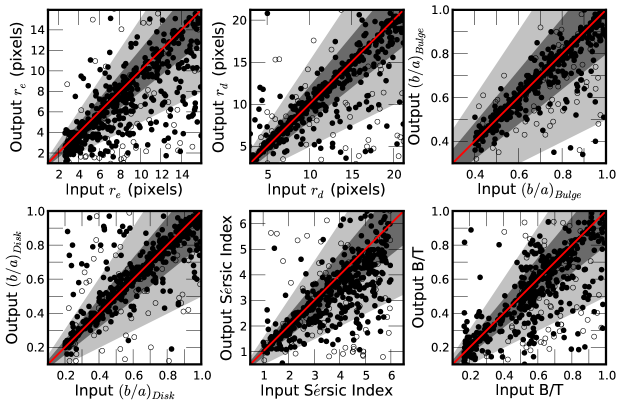
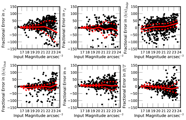
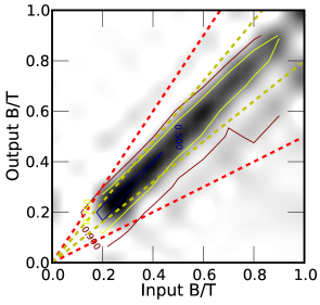
We have used PyMorph to extract parameters from the simulated images. The regression test results are shown in Figure 9. We have calculated the mean magnitude per arcsec2 within the half light radius of the galaxy, which is given by the SExtractor FLUX_RADIUS parameter. We found that for most of the cases the extracted parameters are within a fractional error of 50% for a mean surface brightness arcsec2 (Figure 10). It is found that for 75% objects the recovered parameters are within 20% of the input value. Also for 90% cases the recovered values are within 50% of the inputs. In Figure 11 we show the fraction of recovered within different confidence levels. From that figure it is evident that more than 90% of the galaxies are well within 50% of the input value.
In Figure 9 it can be seen that the bulge parameters are underestimated for some cases. We found that this is largely due to the overestimation of sky value by SEXTRACTOR. Due to this, if we fix the background value at the SEXTRACTOR value while fitting, we obtain incorrect bulge parameters. The result can be improved by leaving the background free (as we have done in our tests), but only a better algorithm to determine the sky can get rid of this problem completely.
5.5 Sensitivity to SEXTRACTOR input parameters
While running Pymorph, the user has some flexibility in choosing input parameters to SEXTRACTOR. It is important to test whether changes in SEXTRACTOR input parameters affects the final results, when processing real data. As a simple test, we used SDSS images of 160 galaxies in the band randomly selected (from within 4 morphological classes in equal numbers) from the catalogue of visualy classified galaxies from Nair & Abraham (2010). Our sample of 160 galaxies includes nearly equal number of all the morphological types (ellipticals, lenticulars, early type spirals, late type spirals). Our galaxies were selected to exclude those with bars/rings or any morphological components, other than bulge and disk.
The input parameters that are likely to change galaxy structural parameters significantly, are those related to the detection threshold and background estimation. Therefore, we checked whether the final output of GALFIT changes significantly as these parameters of SEXTRACTOR are changed. We experimented with a detection threshold varying between 0.5 and 2.0. We checked whether the output varies if one uses GLOBAL background instead of LOCAL. We also varied the size of the background square used in SEXTRACTOR (64 and 128 pixels wide). In all these tests, there was no systematic deviation in extracted parameters, and an overwhelming fraction of galaxies were consistently fit.
6 Parallel PyMorph (PPyMorph)
When one thinks of the amount of data available from large astronomical surveys today and volumes that will be obtained with upcoming surveys, the need for parallisation of astronomical software, whereever feasible, emerges naturally. For the estimation of structural parameters, PyMorph needs significant computational time when operating on large samples. We, therefore implemented PyMorph in the parallel mode to make use of large number of CPUs and process significant amount of data in a short time. The architecture of PPyMorph is simple. It uses the Single Program, Multiple Data technique. In this technique, we send different galaxy data to different processors in a cluster to achieve coarse parallisation. Each processor runs PyMorph on these data, and finally, all the results are collected together. We use the Python pypar module extensively in PPyMorph.
Figure 12 shows the architecture of parallel PyMorph. Here the user has the freedom to give input images in a variety of ways. It is possible to give a large frame(s) which contains several objects or cutouts of objects. In all the cases PPyMorph assigns one processor as the MASTER and that creates cutouts of the galaxies. These are then sent, one by one, to an available processor in the cluster which is called a SLAVE. The SLAVE calls PyMorph to run on this cutout image in galcut mode. While the SLAVE is working on the given cutout, the MASTER searches for an unoccupied SLAVE and assigns another galaxy to it. This continues until all the available SLAVES are engaged. Then MASTER readies cutout of additional galaxies in the list and waits, until one of the SLAVES finishes processing the galaxy assigned to it. When it finds a free SLAVE it fires the next job to that particular SLAVE. This process continues until the MASTER has no more galaxies left to fit. At this stage, the MASTER starts compilation of all the results by the SLAVES and creates final outputs (plots, html, csv etc.) for all galaxies.
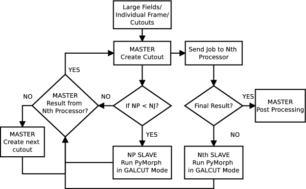
In the non-parallel version, the pipeline takes sec to generate all the structural parameters for a cutout of size on a computer with a Intel Core2 Duo CPU at 1.5GHz with 2GB RAM. In the parallel version, as the number of processors increases 10 fold, the required time decreases fold.
7 Summary
We have presented a new software pipeline, PyMorph, to determine the structural parameters of galaxies in an automated way. We have described the methods implemented in the program. In the best cases, PyMorph uses a relatively small number of user-specified parameters, as compared to traditional fitting procedures. It makes extensive use of SEXTRACTOR and GALFIT. PyMorph tries to obtain a global minimum from GALFIT through clever use of the input parameters. We have tested the program for simulated data and compared our results with earlier published results. To increase processing speed, we have developed a parallel form of the pipeline. Although PyMorph currently employs the popular GALFIT software as the minimisation engine, it is flexible enough to allow the user to replace GALFIT with some other galaxy structural decomposition software, by modifying Pymorph.
The application of PyMorph ranges from individual images to large surveys. We have ourselves used the Pymorph pipeline for a study of galaxy morphology in clusters at moderate redshift (Vikram et al. 2010). Since it is implemented in Python PyMorph is largely OS independent. Also the implementation in Python make the code reusable. PPyMorph makes it possible for astronomers to get structural parameters of a large number of galaxies in a short time. Given the complexity of the Pymorph package, we believe that some users will prefer to use a web enabled interface to Pymorph to obtain structural parameters for their galaxy images, without having to install the full Pymorph package. We are in the process of designing a Virtual Observatory compatible web interface to PyMorph in collaboration with VO-India.
A user manual of PyMorph is available at https://www.iucaa.ernet.in/vvinuv/UsersManual with detailed discussions on the input and output parameters. PyMorph source code is available on request.
Acknowledgments
We thank the anonymous referee for useful comments which have greatly improved this paper. We thank K. Indulekha , Swara Ravindranath and Sajeeth Ninan Philip for useful discussions. Vinu Vikram acknowledges financial support from the Council of Scientific and Industrial Research (CSIR). He also thanks IUCAA for the excellent hospitality provided during this work.
References
- [Abazajian, Adelman-McCarthy, Agüeros, Allam, Allende Prieto, An, Anderson, Anderson, Annis, Bahcall, Bailer-Jones, Barentine, Bassett, Becker, Beers, Bell, Belokurov, Berlind, Berman, Bernardi, Bickerton, Bizyaev, Blakeslee, Blanton, Bochanski, Boroski, Brewington, Brinchmann, Brinkmann, Brunner, Budavári, Carey, Carliles, Carr, Castander, Cinabro, Connolly, Csabai, Cunha, Czarapata, Davenport, de Haas, Dilday, Doi, Eisenstein, Evans, Evans, Fan, Friedman, Frieman, Fukugita, Gänsicke, Gates, Gillespie, Gilmore, Gonzalez, Gonzalez, Grebel, Gunn, Györy, Hall, Harding, Harris, Harvanek, Hawley, Hayes, Heckman, Hendry, Hennessy, Hindsley, Hoblitt, Hogan, Hogg, Holtzman, Hyde, Ichikawa, Ichikawa, Im, Ivezić, Jester, Jiang, Johnson, Jorgensen, Jurić, Kent, Kessler, Kleinman, Knapp, Konishi, Kron, Krzesinski, Kuropatkin, Lampeitl, Lebedeva, Lee, Lee, Leger, Lépine, Li, Lima, Lin, Long, Loomis, Loveday, Lupton, Magnier, Malanushenko, Malanushenko, Mandelbaum, Margon, Marriner, Martínez-Delgado, Matsubara, McGehee, McKay, Meiksin, Morrison, Mullally, Munn, Murphy, Nash, Nebot, Neilsen, Newberg, Newman, Nichol, Nicinski, Nieto-Santisteban, Nitta, Okamura, Oravetz, Ostriker, Owen, Padmanabhan, Pan, Park, Pauls, Peoples, Percival, Pier, Pope, Pourbaix, Price, Purger, Quinn, Raddick, Fiorentin, Richards, Richmond, Riess, Rix, Rockosi, Sako, Schlegel, Schneider, Scholz, Schreiber, Schwope, Seljak, Sesar, Sheldon, Shimasaku, Sibley, Simmons, Sivarani, Smith, Smith, Smolčić, Snedden, Stebbins, Steinmetz, Stoughton, Strauss, Subba Rao, Suto, Szalay, Szapudi, Szkody, Tanaka, Tegmark, Teodoro, Thakar, Tremonti, Tucker, Uomoto, Vanden Berk, Vandenberg, Vidrih, Vogeley, Voges, Vogt, Wadadekar, Watters, Weinberg, West, White, Wilhite, Wonders, Yanny, Yocum, York, Zehavi, Zibetti, & Zucker 2009] Abazajian K. N., Adelman-McCarthy J. K., Agüeros M. A., Allam S. S., Allende Prieto C., An D., Anderson K. S. J., Anderson S. F., et al., 2009, ApJS, 182, 543
- [Abraham, Tanvir, Santiago, Ellis, Glazebrook, & van den Bergh 1996] Abraham R. G., Tanvir N. R., Santiago B. X., Ellis R. S., Glazebrook K., van den Bergh S., 1996, MNRAS, 279, L47
- [Barway, Kembhavi, Wadadekar, Ravikumar, & Mayya 2007] Barway S., Kembhavi A., Wadadekar Y., Ravikumar C. D., Mayya Y. D., 2007, ApJ, 661, L37
- [Barway, Wadadekar, Kembhavi, & Mayya 2009] Barway S., Wadadekar Y., Kembhavi A. K., Mayya Y. D., 2009, MNRAS, 394, 1991
- [Bertin & Arnouts 1996] Bertin E., Arnouts S., 1996, A&AS, 117, 393
- [Byun & Freeman 1995] Byun Y. I., Freeman K. C., 1995, ApJ, 448, 563
- [Conselice 2003] Conselice C. J., 2003, ApJS, 147, 1
- [de Jong 1996] de Jong R. S., 1996, A&AS, 118, 557
- [de Souza, Gadotti, & dos Anjos 2004] de Souza R. E., Gadotti D. A., dos Anjos S., 2004, ApJS, 153, 411
- [Frei, Guhathakurta, Gunn, & Tyson 1996] Frei Z., Guhathakurta P., Gunn J. E., Tyson J. A., 1996, AJ, 111, 174
- [Gadotti 2008] Gadotti D. A., 2008, MNRAS, 384, 420
- [Häussler, McIntosh, Barden, Bell, Rix, Borch, Beckwith, Caldwell, Heymans, Jahnke, Jogee, Koposov, Meisenheimer, Sánchez, Somerville, Wisotzki, & Wolf 2007] Häussler B., McIntosh D. H., Barden M., Bell E. F., Rix H., Borch A., Beckwith S. V. W., Caldwell J. A. R., et al., 2007, ApJS, 172, 615
- [James 1994] James F., 1994, MINUIT: Function Minimization and Error Analysis (CERN Program Libr. Long Writeup D506) (version 94.1; Geneva: CERN)
- [Khosroshahi, Wadadekar, & Kembhavi 2000] Khosroshahi H. G., Wadadekar Y., Kembhavi A., 2000, ApJ, 533, 162
- [Laurikainen, Salo, & Buta 2005] Laurikainen E., Salo H., Buta R., 2005, MNRAS, 362, 1319
- [Lintott, Schawinski, Slosar, Land, Bamford, Thomas, Raddick, Nichol, Szalay, Andreescu, Murray, & Vandenberg 2008] Lintott C. J., Schawinski K., Slosar A., Land K., Bamford S., Thomas D., Raddick M. J., Nichol R. C., et al., 2008, MNRAS, 389, 1179
- [Lotz, Primack, & Madau 2004] Lotz J. M., Primack J., Madau P., 2004, AJ, 128, 163
- [MacArthur, Courteau, & Holtzman 2003] MacArthur L. A., Courteau S., Holtzman J. A., 2003, ApJ, 582, 689
- [Nair & Abraham 2010] Nair P. B., Abraham R. G., 2010, ApJS, 186, 427
- [Peng, Ho, Impey, & Rix 2002] Peng C. Y., Ho L. C., Impey C. D., Rix H., 2002, AJ, 124, 266
- [Peng, Ho, Impey, & Rix 2010] —, 2010, AJ, 139, 2097
- [Press, Teukolsky, Vetterling, & Flannery 1992] Press W. H., Teukolsky S. A., Vetterling W. T., Flannery B. P., 1992, Numerical recipes in C. The art of scientific computing, Press, W. H., Teukolsky, S. A., Vetterling, W. T., & Flannery, B. P. , ed.
- [Ravindranath, Ho, Peng, Filippenko, & Sargent 2001] Ravindranath S., Ho L. C., Peng C. Y., Filippenko A. V., Sargent W. L. W., 2001, AJ, 122, 653
- [Rix, Barden, Beckwith, Bell, Borch, Caldwell, Häussler, Jahnke, Jogee, McIntosh, Meisenheimer, Peng, Sanchez, Somerville, Wisotzki, & Wolf 2004] Rix H., Barden M., Beckwith S. V. W., Bell E. F., Borch A., Caldwell J. A. R., Häussler B., Jahnke K., et al., 2004, ApJS, 152, 163
- [Scoville, Aussel, Brusa, Capak, Carollo, Elvis, Giavalisco, Guzzo, Hasinger, Impey, Kneib, LeFevre, Lilly, Mobasher, Renzini, Rich, Sanders, Schinnerer, Schminovich, Shopbell, Taniguchi, & Tyson 2007] Scoville N., Aussel H., Brusa M., Capak P., Carollo C. M., Elvis M., Giavalisco M., Guzzo L., et al., 2007, ApJS, 172, 1
- [Sersic 1968] Sersic J. L., 1968, Atlas de galaxias australes, Sersic, J. L., ed.
- [Simard 1998] Simard L., 1998, in Astronomical Society of the Pacific Conference Series, Vol. 145, Astronomical Data Analysis Software and Systems VII, R. Albrecht, R. N. Hook, & H. A. Bushouse, ed., pp. 108–+
- [Simard, Willmer, Vogt, Sarajedini, Phillips, Weiner, Koo, Im, Illingworth, & Faber 2002] Simard L., Willmer C. N. A., Vogt N. P., Sarajedini V. L., Phillips A. C., Weiner B. J., Koo D. C., Im M., et al., 2002, ApJS, 142, 1
- [Skrutskie, Cutri, Stiening, Weinberg, Schneider, Carpenter, Beichman, Capps, Chester, Elias, Huchra, Liebert, Lonsdale, Monet, Price, Seitzer, Jarrett, Kirkpatrick, Gizis, Howard, Evans, Fowler, Fullmer, Hurt, Light, Kopan, Marsh, McCallon, Tam, Van Dyk, & Wheelock 2006] Skrutskie M. F., Cutri R. M., Stiening R., Weinberg M. D., Schneider S., Carpenter J. M., Beichman C., Capps R., et al., 2006, AJ, 131, 1163
- [Vikram, Wadadekar, Kembhavi, & Vijayagovindan 2010] Vikram V., Wadadekar Y., Kembhavi A. K., Vijayagovindan G. V., 2010, MNRAS, 401, L39
- [Wadadekar, Robbason, & Kembhavi 1999] Wadadekar Y., Robbason B., Kembhavi A., 1999, AJ, 117, 1219
- [York, Adelman, Anderson, Anderson, Annis, Bahcall, Bakken, Barkhouser, Bastian, Berman, Boroski, Bracker, Briegel, Briggs, Brinkmann, Brunner, Burles, Carey, Carr, Castander, Chen, Colestock, Connolly, Crocker, Csabai, Czarapata, Davis, Doi, Dombeck, Eisenstein, Ellman, Elms, Evans, Fan, Federwitz, Fiscelli, Friedman, Frieman, Fukugita, Gillespie, Gunn, Gurbani, de Haas, Haldeman, Harris, Hayes, Heckman, Hennessy, Hindsley, Holm, Holmgren, Huang, Hull, Husby, Ichikawa, Ichikawa, Ivezić, Kent, Kim, Kinney, Klaene, Kleinman, Kleinman, Knapp, Korienek, Kron, Kunszt, Lamb, Lee, Leger, Limmongkol, Lindenmeyer, Long, Loomis, Loveday, Lucinio, Lupton, MacKinnon, Mannery, Mantsch, Margon, McGehee, McKay, Meiksin, Merelli, Monet, Munn, Narayanan, Nash, Neilsen, Neswold, Newberg, Nichol, Nicinski, Nonino, Okada, Okamura, Ostriker, Owen, Pauls, Peoples, Peterson, Petravick, Pier, Pope, Pordes, Prosapio, Rechenmacher, Quinn, Richards, Richmond, Rivetta, Rockosi, Ruthmansdorfer, Sandford, Schlegel, Schneider, Sekiguchi, Sergey, Shimasaku, Siegmund, Smee, Smith, Snedden, Stone, Stoughton, Strauss, Stubbs, SubbaRao, Szalay, Szapudi, Szokoly, Thakar, Tremonti, Tucker, Uomoto, Vanden Berk, Vogeley, Waddell, Wang, Watanabe, Weinberg, Yanny, & Yasuda 2000] York D. G., Adelman J., Anderson Jr. J. E., Anderson S. F., Annis J., Bahcall N. A., Bakken J. A., Barkhouser R., et al., 2000, AJ, 120, 1579