Gravity/Spin-model correspondence and holographic superfluids

Abstract:

We propose a general correspondence between gravity and spin models, inspired by the well-known IR equivalence between lattice gauge theories and the spin models. This suggests a connection between continuous type Hawking-phase transitions in gravity and the continuous order-disorder transitions in ferromagnets. The black-hole phase corresponds to the ordered and the graviton gas corresponds to the disordered phases respectively. A simple set-up based on Einstein-dilaton gravity indicates that the vicinity of the phase transition is governed by a linear-dilaton CFT. Employing this CFT we calculate scaling of observables near $T_{c}$, and obtain mean-field scaling in a semi-classical approximation. In case of the XY model the Goldstone mode is identified with the zero mode of the NS-NS two-form. We show that the second speed of sound vanishes at the transition also with the mean field exponent.

1 Introduction

There has been great progress recently in applications of holography [1, 2, 3] to condensed matter systems such as superconductors following the pioneering works of [4] and [5]. These authors managed to find a simple gravitational background in Einstein-Maxwell gravity coupled to a complex scalar field where a second order normal-to-superfluid type transition occurs at finite temperature. The basic interest behind application of holographic ideas to condensed matter theory (CMT) lies in the hope that the strongly correlated condensed matter systems may secretly possess a gravitational description. Indeed, computations of certain observables in the gravity picture, such as conductivity provides supporting evidence, see [6][7][8] for reviews. It is a considerable possibility that [9] the underlying dynamics behind the phase transition in high $T_{c}$ superconducting materials is a strongly coupled quantum phase transition at zero T. Then the hope is that, a dual gravity description of the strongly coupled field theory around this critical point may also shed light over the finite temperature transition in the quantum critical region.

On the other hand, there are several issues of fundamental importance in the proposed gravity-CMT models, such as the role of the large N limit and the notion of weak-strong duality, that are not entirely clarified. We have a much better understanding in the holographic constructions of gauge theories, thanks to the basic example [1, 2, 3] of the ${\cal N}=4$ super Yang-Mills theory where the D3 brane picture provide the link between the gauge side and the gravity side. Such a “top-bottom” approach is missing in the gravity-CMT models.

In this work, we entertain the possibility that such a link may be established under certain assumptions, at least for certain simple condensed matter systems, i.e. spin models, by analogy with the better understood gauge-gravity case.

The building blocks of such a connection are already present in the well-known literature. First of all, we recall the famous equivalence between lattice gauge theories (LGT) and spin-models (SpM)[10, 11]: Integrating out the gauge invariant degrees of freedom in the partition function of a LGT with gauge group $G$, one arrives at an effective action for the lowest lying mode, namely the Polyakov loop $P$. This effective action is invariant under the leftover center symmetry ${\cal C}=Center(G)$ of the original gauge invariance. Identifying the Polyakov loop $P$ with a spin field $\vec{s}$, one then obtains the partition function of a spin-model with the global spin invariance ${\cal C}$. Using this equivalence between lattice gauge theories and spin-models Polyakov and Susskind were able to show the existence of confinement-deconfinement phase transition on the lattice, long time ago. Based on these works, than Svetitsky and Yaffe [12] further proposed that, if continuous critical phenomena prevails in the continuum limit of a certain lattice gauge theory, then it should fall in the same universality class as the corresponding spin-model.

It is interesting to employ the same idea in the opposite direction in order to study a spin-model that is strongly coupled at criticality. In particular, one would like to compute the critical exponents, the transition temperature $T_{c}$, certain thermodynamic functions etc., by analytic methods. If one is lucky enough to find a gauge-theory that corresponds to the spin-model under the aforementioned equivalence, then one may be able to study the strongly coupled phenomena by the gauge-gravity correspondence.

One purpose of this paper is to emphasize that this chain of dualities may provide a well-defined setting in understanding fundamental issues in the gravity-CMT correspondence. In particular, if one can figure out the relevant D-brane configuration that describes the gauge theory which arises in the continuum limit of the LGT under question, then one may be able to take the decoupling limit and obtain a gravity description of the LGT—and of the equivalent spin model—around criticality. Despite being abstract, in principle this provides a top-bottom approach to the problem. In particular, such an approach would hopefully provide a microscopic description that is long sought for in holographic applications to CMT.

Another purpose of this paper is to provide a concrete realization of these ideas in a simple setting. For this purpose we consider $SU(N)$ gauge theory in $d$-dimensions (with possible adjoint matter) in the strict $N\to\infty$ limit. In this limit the center ${\cal C}$ becomes $U(1)$. We imagine that the adjoint matter is arranged such that the deconfinement transition of the gauge theory is of continuous type. This transition is then in the same universality class with the order-disorder transition in the corresponding $U(1)$ rotor model in $d-1$ dimensions—that is sometimes called the XY model. The XY-models—and their $O(n)$ generalizations—provide canonical examples of superfluidity that arises as spontaneous breaking of the global $U(1)$ symmetry in a continuous phase transition.

To realize this phenomenon in the dual gravity setting we consider the NS-NS sector of non-critical string theory in $d+1$ dimensions with Euclidean time direction $x^{0}$ compactified. It was shown in [15] that this theory in the two-derivative sector exhibits a continuous Hawking-Page transition at some finite temperature $T_{c}$. The background is of the type $AdS^{d+1}$ near the boundary and linear-dilaton in the deep-interior. Building upon the ideas in [13], we argue that the $U(1)$ symmetry (in the strict $N\to\infty$ limit) corresponds to the shift symmetry $\int_{M}B\to\int_{M}B+const$ where $B$ is the NS-NS two-form field and $M$ is the $(r,x^{0})$ subspace of the background geometry. The only objects that are charged under this symmetry are string states winding the time circle. In the thermal gas phase these states have infinite energy and cannot be excited, hence the symmetry is unbroken and this phase corresponds to the normal phase of the spin system. In the black-hole phase on the other-hand they have finite energy (with an appropriate regularization) and the black-hole corresponds to the superfluid phase.

It was further observed in [15] that the geometry becomes exactly linear-dilaton in the transition region. Therefore, we argue that the transition region of the XY model is governed by the linear-dilaton CFT on the string side. Although in general the $\alpha^{\prime}$ corrections can not be ignored in the type of backgrounds that we will consider in this paper, one can still perform calculations in the critical regime, precisely because the linear-dilaton background is known to be an $\alpha^{\prime}$-exact background in non-critical string theory[16]. In particular the calculations that involve probe strings can be performed by employing the exact CFT description of the linear-dilaton background, (in the limit $g_{s}\to 0$).

The spin operator $\vec{s}(x)$ is related to a fundamental string that wraps the time-circle and connected to the boundary at point $x$. Consequently one can compute correlation functions of the operator $\vec{s}$ by studying the string propagation in the linear-dilaton CFT in the (single) winding sector. We perform such calculations in a semi-classical limit where we only take into account the contribution of the lowest-lying string states. It is shown that in this approximation, one obtains mean-field scaling near $T_{c}$. We find that the “magnetization” behaves as

$$M\sim(T-T_{c})^{\frac{1}{2}},\qquad as,\,\,\,T\to T_{c}.$$

A similar calculation with string propagation connecting the points $x$ and $y$ on the (spatial) boundary corresponds to the spin two-point function. We show that the expected behavior of the spin-system arises in the large $|x-y|$ limit near $T_{c}$ indeed arises from this calculation in a non-trivial manner. In particular, in order to show that the correlation length $\xi$ diverges at $T_{c}$, one has to identify the transition with the Hagedorn temperature where the lowest lying single-winding mode becomes massless [17]. With such an identification one indeed finds the expected behavior

$$\xi\sim(T-T_{c})^{-\frac{1}{2}},\qquad as,\,\,\,T\to T_{c},$$

again in a semi-classical approximation.

One can also study scaling of the speed of second sound that is associated with the Goldstone mode in the superfluid phase. This mode is identified with fluctuations of the zero-mode of the $NS$ two-form field $B$. We find that the speed of sound indeed vanishes at $T_{c}$ precisely with the expected mean-field scaling,

$$c_{s}^{2}\sim(T-T_{c}),\qquad as\,\,\,T\to T_{c}$$

in a second order Hawking-Page transition. We also argue that this finding is not altered by possible $\alpha^{\prime}$ corrections.

The identification of spin operators with the F-strings suggest a similar identification between the vortex configurations—that play an important role in the 2D XY model—with D-strings in the gravity dual. We study correlation functions of such D-string configurations and find that they exhibit the expected behavior in the spin-model.

The paper is organized as follows. In the next section, we review basic ideas in the past literature which indicate a general duality between spin-systems and gravity. We first focus on the case of $SU(N)$ in the $N\to\infty$ limit and postpone the general discussion to section 6. Section 3 reviews the Einstein-dilaton system that was studied in [15]. In section 4 we argue that the IR limit of the model is described by a linear-dilaton CFT and review basic features of such CFTs. Section 5 contains main technical results of this paper. We first review the basic statistical mechanics results that are relevant in what follows. Then we propose the precise identification between the F-string configurations and the spin correlation functions. We calculate the one-point and two-point functions near criticality in the semi-classical approximation making use of the linear-dilaton CFT. Finally we present calculations related to vortex configurations. In section 6 we take a first step in formulating a gravity spin-model duality in general. In the last section we discuss various issues and possible future directions of research.

Several appendices detail our presentation. In appendix A, we review the simplest example od the equivalence between lattice gauge theories and the spin-systems. In appendix B, we review the connection between non-critical string theory and the linear-dilaton background. Appendix C provides some basic background material in statistical mechanics of the XY models for the unfamiliar reader. Finally, Appendices D and E contain details of our calculations in section 5.

2 Gravity - spin model duality

Our goal in this section is to propose a particular approach to the gravity-CMT correspondence that relates the spin-models in CMT to gravity by a two step procedure: The first step is to employ a well-known equivalence between spin-models and lattice gauge theories [10, 11] followed by a second step that is to utilize the gauge-gravity duality to relate the (continuum limit) of the lattice gauge theory to a dual gravitational background.

2.1 Correspondence between gauge theories and spin systems

Existence of the confinement-deconfinement phase transition in lattice gauge theories at strong coupling is rigorously proved [10, 11] long time ago. The proof is based on an equivalence between lattice gauge theories (LGT) and spin systems with nearest-neighbor ferromagnetic interactions, [10, 11, 12]. In the original papers of Polyakov and Susskind, this equivalence was established for the cases of $U(1)$ and $SU(2)$ gauge theories. Subsequently it was generalized to general Lie groups. We shall refer to this equivalence as the LGT-spin model equivalence. We review how the spin systems arise from the lattice gauge theories in the Hamiltonian formalism, and in the simplest case of $U(1)$ gauge group in Appendix A.

This equivalence has profound implications in the continuum limit: As argued and verified with various examples by Svetitsky and Yaffe [12], the critical phenomena—if exists—in the continuum limit of the LGT, should be in the same universality class with the corresponding spin model. Therefore, a continuous order-disorder type transition in a $d-1$ dimensional spin-model with global symmetry group ${\cal C}$ is directly related to a continuous type confinement-deconfinement transition of the gauge theory with gauge group $G$ where ${\cal C}=Center(G)$.

Let us briefly review the argument of [12]. The basic observation is that the magnetic fluctuations are always gapped both in the high and the low T limit of the lattice gauge theory. Therefore, they are expected to be gapped for any T on a trajectory crossing the phase boundary in figure 1. This means that the magnetic fluctuations should not play an essential role at criticality in the vicinity of a continuous confinement-deconfinement transition. Integrating these short-range fluctuations, one indeed obtains an effective theory that only involves the Polyakov loops, which in turn can be mapped on a spin model. Therefore the critical phenomena, e.g. the critical exponents etc. of the lattice gauge theory around a continuous transition should be governed by the corresponding spin model.

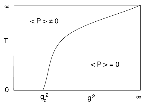
Figure 1: Typical phase diagram of a lattice gauge theory with non-trivial center. Low T phase is confining with vanishing expectation value for the Polyakov loop $P$ and high T phase is de-confined. We assume that (at least a portion) of the phase boundary that separates these phases is of second or higher order. Then the critical phenomena around the phase boundary is determined by the corresponding spin-model.

The magnetic sector is gapped at low T by assumption. We assume that the (bare) coupling constant is large enough (see figure 1) so that the low T theory is confined. The argument at high T is as follows. In the Lagrangian formulation of the LGT one can take the action to be,

$${\cal A}_{lgt}=\sum_{\vec{r}}{\rm Re}\left\{\beta_{t}\sum_{i}{\rm Tr}U_{\vec{r},0i}+\beta_{s}\sum_{ij}{\rm Tr}U_{\vec{r},ij}\right\};\qquad U_{\vec{r},\mu\nu}=U_{\vec{r},\mu}U_{\vec{r}+\hat{\mu},\nu}U^{\dagger}_{\vec{r}+\hat{\nu},\mu}U^{\dagger}_{\vec{r},\nu}$$ (2.1)

where $\vec{r}$ labels sites on the square lattice, $U_{\vec{r},\mu\nu}$ are the product of link variables on a plaquette with corner $\vec{r}$. The first term in the action above corresponds to the electric contribution and the second to the magnetic. The electric and magnetic coupling constants are related to the bare coupling constant of the LGT and the temperature as follows:

$$\frac{2}{g^{2}}=a^{4-d}\sqrt{\beta_{t}\beta_{s}},\qquad T=\sqrt{\frac{\beta_{t}}{\beta_{s}}}\frac{1}{N_{t}a}$$ (2.2)

where $a$ is the lattice spacing and $N_{t}$ is the number of the lattice sites in the Euclidean time direction. One observes that, at fixed coupling, $\beta_{t}\sim T$. Then, for sufficiently high T, only configurations with vanishing electric flux contributes in the partition function. This reduces the system to static configurations at high T, hence the theory can be thought of a $d-1$ dimensional LGT at zero T, with a coupling constant $g^{2}_{d-1}=g^{2}_{d}T$. Any such LGT with a non-trivial center is confined and exhibits magnetic screening at strong coupling [12]. As mentioned before, the equivalence to the spin-models can be shown exactly at strong coupling, [10, 11].

Svetitsky and Yaffe [12] were able to make reliable predictions concerning the critical phenomena of a wide range of lattice gauge theories making use of this connection and the well-known results on the critical phenomena of the corresponding spin-models.

First of all, they correctly predicted that the 2nd order transition in the pure $SU(2)$ theory in 4D is in the same universality class with the 3D Ising model (see e.g. [19] and references therein). As another check of these arguments [12] presents the example of $SU(N)$ theory for $d-1=2$, $N>4$ where the dual spin model is again $Z_{N}$ symmetric and exhibit a BKT type continuous transition. In this case, it was argued that for large N , the theory approximates that of a $U(1)$ LGT in 2+1 and the corresponding spin-model should be the XY-model in 2D. It was explicitly checked in [12] that, for the $U(1)$ LGT the critical phenomena is in the same universality class as that of the 2D XY model. More generally, if the $d=2+1$ $SU(N)$ gauge theory—or a suitable deformation with additional adjoint matter—involves continuous critical phenomena than it should be the BKT type.

A particularly interesting case concerns $SU(N)$ gauge theory in $d-1>2$ spatial dimensions with $N>4$ (that includes the large $N$) where the dual spin model is $Z_{N}$ symmetric. We then consider the large N limit that is most relevant for the gauge-gravity duality. It is reasonable to believe that in the strict $N\to\infty$ limit (with or without adjoint matter), the center $Z_{N}$ is promoted to $U(1)$. See [13] for an argument in favor of this, in the case of ${\cal N}=4$ SYM at strong-coupling. Another indication that this happens in $Z_{N}$ invariant LGT at $d=2$ is explained in [12]. Therefore, by the universality arguments above, if there exist a continuous phase transition it should be governed by a $U(1)$ invariant spin model .

We review how the equivalence of LGTs and spin-systems work at strong coupling in Appendix A for the unfamiliar reader. Here we shall mention two salient features.

• The temperature of the spin-system is inversely related to temperature in the original gauge theory:

  $$T_{s}\sim T_{l}^{-1}.$$ (2.3)

  Consequently, the low temperature (confined) phase of the gauge theory corresponds to the high temperature (disordered) phase of the ferromagnet, whereas the high temperature (de-confined) phase of the gauge theory corresponds to the low temperature (ordered) phase of the ferromagnet.

• Quite generally, the LGT-spin model equivalence can be generalized to incorporate (adjoint) matter. This is mainly because the basic ingredient in the calculation i.e. the center symmetry of the LGT remains intact upon addition of adjoint matter. See [14] for a related recent discussion.

2.2 Holographic superfluidity

Here and until section 6, we specify to the particular case of $U(1)$ invariant spin-models. Continuous critical phenomena in such models include the interesting case of superfluidity, that requires spontaneous breaking of the global $U(1)$ symmetry. As reviewed above this transition is directly connected to the confinement-deconfinement transition in the gauge theory. In the original derivation of [10][11], the de-confined phase of the $U(1)$ invariant LGT was understood as an ordered phase of the $U(1)$ spin model. This is clear from the discussion of section 2, as the center of $U(1)$ is $U(1)$ itself.

Instead, here we shall adopt an alternative approach where the $U(1)$ factor arises from the large N limit of an $SU(N)$ gauge theory (pure or with adjoint matter). In this case the deconfinement transition can be understood in the gravity dual as a Hawking-Page transition by a generalization of the arguments in [13]. Assuming that the following assumptions hold,

• There exists a suitable $SU(N)$ lattice gauge theory with coupling to adjoint matter chosen such that, at large N it flows to an IR fixed point with a continuous confinement-deconfinement transition,

• Gauge-gravity correspondence holds and maps this to a Hawking-Page type transition,

then one should be able to map the normal-to-superfluid transition in the XY model to a continuous Hawking-Page type transition on the gravity side.

The $U(1)$ symmetry of the spin-model follows on the GR side from the shift symmetry $\psi\to\psi+const.$ where $\psi$ is the flux of the B-field

$$\psi=\int_{M}B={\rm const.}$$ (2.4)

on the subspace $M$ of the BH geometry that is spanned by the coordinates r and $x_{0}$. In this paper we consider gravitational set-ups where the B-field is either constant or pure gauge $B=d\xi$ so that it does not back-react on the solution with $H=dB=0$. Of course such a B-field has no visible effect on the gravitational solution and in the second case it can be removed by a gauge transformation. This ceases to be the case in presence of objects that are charged under this shift symmetry.

In the classical approximation where one keeps only the low-lying gravity fields, there are no bulk fields that carry the extra $B$ charge. However, strings that wind around the time-circle couple to the B-field through the term $i\psi$, thus they are charged under the shift symmetry with the identification $\psi\sim\psi+2\pi$. We shall denote this topological $U(1)$ symmetry as $U(1)_{B}$ Therefore a non-vanishing string one-point function signals a breakdown of the $U(1)_{B}$ symmetry. On the spin-model side this corresponds to an order-disorder transition upon identification of the $U(1)_{B}$ symmetry with the $U(1)$ spin symmetry of the spin-model. Below, we would like to review these ideas in more detail.

2.3 Spontaneous breaking of $U(1)_{B}$, the Goldstone mode and the second speed of sound

For simplicity, let us consider the (critical or non-critical) bosonic string theory on a background with $U(1)\times E(d-1)$ isometry where the $U(1)$ corresponds to the temporal $S^{1}$, and $E(d-1)$ to translations and rotations on the spatial part. The general background with these symmetries is of the form

$$ds^{2}=A(r,\Omega)dx_{0}^{2}+B(r,\Omega)dK^{2}+C(r,\Omega)dr^{2}+D(r,\Omega)d\Omega;\quad\overline{\Phi}=\overline{\Phi}(r,\Omega)\quad H=dB=0,$$ (2.5)

where $x_{0}\sim x_{0}+1/T$, $K$ is the $d-1$ dimensional transverse part, and $\Omega$ is some internal compact manifold. There can be additional bulk fields but we are only interested in the NS-NS sector.

Most of the following traces the arguments in [13]. The order parameter for the transition is the vev of the Polyakov loop, $\langle P[C]\rangle$, where $C$ is a loop isomorphic to the time-circle. This maps to the expectation value of the F-string path integral,

$$\langle P[C]\rangle\propto\langle{\cal W}_{F}\rangle_{SG}$$ (2.6)

where ${\cal W}_{F}$ denotes the F-string path integral over all of the string configurations with the boundary ending on $C$, and the final averaging is path integral over the super-gravity fields that couple to the string. The string path integral is

$${\cal W}_{F}=\int{\cal D}X_{\mu}{\cal D}h_{ab}~{}e^{-\int(G+iB+\overline{\Phi}R^{(2)})},$$ (2.7)

where $R^{(2)}$ is the Ricci scalar on the sub-manifold $M$ that the F-string wraps and $X_{\mu}$ denotes the matter fields. We also use the short-hand notation

$$G\equiv\sqrt{det~{}h_{ab}}~{}h^{ab}\partial_{a}X^{\mu}\partial_{b}X^{\nu}G_{\mu\nu},\qquad B\equiv\sqrt{det~{}h_{ab}}~{}\epsilon^{ab}\partial_{a}X^{\mu}\partial_{b}X^{\nu}B_{\mu\nu}.$$ (2.8)

One has to make sure that ${\cal W}$ is finite by an appropriate regularization of infinite volume of the space time and factoring out diffeo-Weyl gauge volume a la Faddeev-Popov.

In the original discussion of [13] ${\cal W}$ is dominated by the classical saddles that minimize the action in (2.7). The boundary condition for these classical strings is such that at $\tau=0$, $X^{\mu}(\sigma,\tau)$ ends on the temporal circle $x_{0}$, some point x in $K$ and at the cut-off of the radial coordinate $r=\epsilon$.

The string path integral is dominated by classical saddles when $\ell/\ell_{s}\gg 1$ where $\ell$ is the typical curvature of the target space and $\ell_{s}$ is the string length. In the original AdS/CFT correspondence this ratio is proportional to the t ’Hooft coupling of the dual ${\cal N}=4$ SYM theory, $\ell/\ell_{s}\propto\lambda^{\frac{1}{4}}$ and indeed the classical strings dominate in the limit of strong interactions. In the general case here one has to consider the full path integral.

The vev of $P[C]$ is given by the path integral of ${\cal W_{F}}$ over the super-gravity fields that couple the F-string, weighted by the SG action. The non-trivial SG fields are the space-time metric $G_{\mu\nu}$, the B-field $B_{\mu\nu}$ and the dilaton $\overline{\Phi}$. Thus one has,

$$\langle P[C]\rangle\propto\int{\cal D}G_{\mu\nu}~{}{\cal D}B_{\mu\nu}~{}{\cal D}\overline{\Phi}~{}e^{-{\cal A}_{sg}}{\cal W}_{F},$$ (2.9)

where ${\cal A}_{sg}$ is the gravity action. As we are interested in the large N limit of the dual field theory, we can send the string coupling $g_{s}\to 0$ and the SG path integral is dominated by the classical saddles of ${\cal A}_{sg}$. For given asymptotic boundary conditions of $G$, $\overline{\Phi}$ and $B$, the saddles of interest involve only two type of solutions, the thermal gas (TG) and the black-hole (BH). At an arbitrary temperature T (that partially determines the asymptotic boundary condition for $G$), only one of these saddles will dominate the SG path integral as a result of the classical limit $g_{s}\to 0$.

Let us assume that TG dominates at $T<T_{c}$ and BH dominates at $T>T_{c}$. Let us also assume that the BH solution only exists above a certain temperature $T_{min}$. Backgrounds that exhibit confinement generically satisfy $T_{c}\geq T_{min}$ [25, 26]. As explained in detail in [15] and reviewed in the next section, only in the case $T_{min}=T_{c}$ the transition is second or higher order.

On the TG phase, the classical world-sheet $M$ has infinite area. Therefore the string path-integral ${\cal W_{F}}$, hence $\langle P[C]\rangle$ in (2.9) vanishes. One concludes that the TG solution is $U(1)_{B}$ symmetric and the center in the dual gauge theory is unbroken. This means that the dual spin-model is in the normal (disordered) phase. This is precisely as one expects from the behavior of the dual spin model in the high temperature phase, recalling that the temperature of the spin model is inversely proportional to the temperature on the gravity side $T_{s}\propto T^{-1}$.

On the BH solution $T>T_{min}$ however, the classical string saddle $M$ has finite area and one has to evaluate (2.9) carefully. One has to include all of the configurations over the classical fields $G,B$ and $\overline{\Phi}$ with the same on-shell value of the SG action.

The path integral over $G$ and $\overline{\Phi}$ in (2.9) is replaced by the classical solution (2.5) that is a BH in this case. Sum over these saddles include the following important contribution from the B-field. In the black-hole case the sub-manifold M has finite area and the B-field has a flux $\psi=\int_{M}B$. $\psi$ in (2.7) has angular nature because it appears with a factor of i and it can attain any value in the range $\psi\sim\psi+2\pi$. This identification yields the $U(1)_{B}$ invariance. The sum over classical saddles then should include various different values of $\psi$. As $dB=0$ all different values of $\psi$ yield the same on-shell gravity action.

We can thus write,

$$P[C]\propto\int{\cal D}\psi e^{-S_{sg}[\psi]}\int{\cal D}X_{\mu}~{}{\cal D}h_{ab}~{}e^{i\psi}~{}e^{-\int_{M}(G+\overline{\Phi}R^{(2)})},$$ (2.10)

where $S_{sg}$ now is evaluated on the saddle solution and is only a functional of $\psi$. On the other hand the $\psi$ path integral includes the classical saddle $\psi=const$ and the fluctuations $\delta\psi(K)$ around it.

When $K$ is non-compact and $dim(K)>2$, then the fluctuations $\delta\psi(K)$ viewed as a massless bosonic field on $K$ has long-range order, hence $\psi$ should condense. Thus, on the black-hole solution the $U(1)_{B}$ symmetry breaks down. This happens exactly at the point where the black-hole forms, right above $T_{min}$. As a result, the fluctuation $\delta\psi$ in (2.10) becomes a Goldstone mode on the transverse space $K$.

Considering the wave equation for $\delta\psi$ one expects to find,

$$\omega^{2}=c_{\psi}^{2}(T)~{}{\bf q}^{2}+{\cal O}({\bf q}^{4}),$$ (2.11)

where $c_{\psi}$ is the speed of sound of $\psi$ and there is no mass term for $\psi$ for $T>T_{c}$. It is well-known that (see appendix C for a review, and section 5.6 for a holographic derivation in gravity), the speed of sound $c_{\psi}$ of the Goldstone mode vanishes continuously as one approaches the transition temperature $T_{c}$ from above, only if the transition is of continuous type. This is exactly what happens in super-fluidity, where the “second speed of sound”, i.e. the speed of sound associated with the entropy waves vanish as one approaches $T_{c}$ of the XY model from below (recall that temperature in gravity and in the XY model are inversely related). In order to mimic this property of the spin model, we should require that the Hawking-Page transition in gravity is of continuous type, hence $T_{c}=T_{min}$ [15]. In section 5.6 we show by an explicit gravity calculation that indeed the second sound vanishes with the expected mean-field exponents.

Our conclusion is: whenever a second order (or higher order) Hawking phase transition occurs in the gravitational background, it is natural to associate it with super-fluidity. Here the thermal gas phase is dual to the normal phase of the system, and the black-hole phase is dual to the super-fluid. The “first speed of sound” i.e. the sound of the density waves is associated with the graviton fluctuations (that we are considered in [15]), and the “second speed of sound” is associated with the fluctuations of the B-field that we consider in section 5.6.

Lattice gauge theory	Gravity		Spin model
Deconfined, $U\!\!(1)_{\cal C}\!\!\!\!\!\!\!\!\!\!\!\!\!/$	Black-hole, $U\!\!(1)_{B}\!\!\!\!\!\!\!\!\!\!\!\!\!/$		Superfluid , $U\!\!(1)_{S}\!\!\!\!\!\!\!\!\!\!\!\!\!/$
Confined, $U\!\!(1)_{\cal C}$	Thermal gas, $U\!\!(1)_{B}$		Normal phase, $U\!\!(1)_{S}$

One can summarize the various phases of the theories by the table above. The various $U(1)$ factors in this table are as follows: The $U(1)_{B}$ is the dual symmetry that arises from compactifying the B field on the temporal circle. The $U(1)_{\cal C}$ is the center symmetry of the corresponding lattice gauge theory that is proposed to arise in the large N limit of $SU(N)$ (with or without) adjoint matter. Finally the $U(1)_{S}$ is the spin symmetry of the corresponding XY model. The arrow of increasing T is the same for the LGT and gravity picture and opposite in the spin model picture.

3 A model based on Einstein-scalar gravity

The arguments put forward in favor of a gravity-spin model correspondence above are general. In this section we would like to introduce a simple set-up which allows for computations of quantities such as the scaling of magnetization and spin-spin correlation function on the gravity side. The model is inspired by non-critical string theory and it becomes precisely non-critical string theory in the interesting regime near the continuous phase transition.

3.1 The model

The action in the Einstein frame reads,

$${\cal A}=\frac{1}{16\pi G_{N}}\int d^{d+1}x\sqrt{-g}\left(R-\frac{4}{d-1}(\partial\Phi)^{2}+V(\Phi)-\frac{1}{12}e^{-\frac{8}{d-1}\Phi}H^{2}+\cdots\right)+\,\,\,G.H.$$ (3.12)

where the kinetic terms of the dilaton and the B-field $H=dB$ are inspired by non-critical string theory in $d+1$ dimensions. The ellipsis denote higher derivative corrections. The last term in (3.12), that we shall not need to specify here, is the Gibbons-Hawking term on the boundary.

We allow for a non-trivial dilaton potential $V(\Phi)$ that should be specified by matching the thermodynamics of the dual field theory. In the case of non-critical string theory in $d+1$ dimensions the potential is given by,

$$V_{nc}(\Phi)=\frac{\delta c}{\ell_{s}^{2}}e^{\frac{4}{d-1}\Phi},$$ (3.13)

where $\ell_{s}$ is the string length and $\delta c$ is the central deficit, see section 3.3 for more detail. $G_{N}$ in (3.12) is the Newton’s constant in $D=d+1$ dimensions. It is related to N of the dual field theory by,

$$\frac{1}{16\pi G_{N}}=M_{p}^{d-1}N^{2},$$ (3.14)

where $M_{p}$ is a “normalized” Planck scale, that is generally of the same order as the typical curvature of the background $\ell$. The limit of large $N$ corresponds to classical gravity as usual. One should be careful in attaining this classical limit: The correct way of achieving this is described in section 3.3. On the gravity side the parameter N arises from the RR-sector, where it is the integration constant of a space-filling $F_{(d+1)}$ form, $F_{(d+1)}\propto N$. Then the large N limit is defined as sending this value to infinity and sending the boundary value of the dilaton $\Phi_{0}$ to $-\infty$ such that $N\exp(\Phi_{0})$ remains constant and yields $M_{p}$ in (3.14). We refer to section 3.3 for details.

In what follows we shall only consider solutions with either constant or pure-gauge $B$-field whose legs are taken to lie along r and $x_{0}$ directions:

$$B_{\mu\nu}=B_{r0},$$ (3.15)

In this case $H=0$ in (3.12) and the B-field contributes to neither the equations of motion nor the on-shell value of the action. However, it contributes the F-string and D-string solutions as we study in section 5.

There are only two types of backgrounds at finite T (with Euclidean time compactified), with Poincaré symmetries in $d-1$ spatial dimensions, and an additional $U(1)$ symmetry in the Euclidean time direction. These are the thermal graviton gas,

$$ds^{2}=e^{2A_{0}(r)}\left(dr^{2}+dx_{d-1}^{2}+dx_{0}^{2}\right),\qquad\Phi=\Phi_{0}(r),$$ (3.16)

and the black-hole,

$$ds^{2}=e^{2A(r)}\left(f^{-1}(r)dr^{2}+dx_{d-1}^{2}+dx_{0}^{2}f(r)\right),\qquad\Phi=\Phi(r).$$ (3.17)

We define the coordinate system such that the boundary is located at $r=0$. For the potentials $V$ that we consider in this paper, there is a curvature singularity in the deep interior, at $r=r_{s}$. In (3.16), r runs up to singularity $r_{s}$. In (3.17) there is a horizon that cloaks this singularity at $r_{h}<r_{s}$ where $f(r_{h})=0$. $x_{0}$ is the Euclidean time that is identified as $x_{0}\sim x_{0}+1/T$. This defines the temperature T of the associated thermodynamics. In the black-hole solution, the relation between the temperature and $r_{h}$ is obtained in the standard way, by demanding absence of a conical singularity at the horizon:

$$4\pi T=-f^{\prime}(r_{h}).$$ (3.18)

This identifies T and the surface gravity in the BH solution.

In the r-frame defined by (3.16) and (3.17) one derives the following Einstein and scalar equations of motion from (3.12):

$$A^{\prime\prime}-A^{\prime 2}+\frac{\xi}{d-1}\Phi^{{}^{\prime}2} = 0,$$ (3.19)

$$f^{\prime\prime}+(d-1)A^{\prime}f^{\prime} = 0,$$ (3.20)

$$(d-1)A^{\prime 2}+A^{\prime}f^{\prime}+A^{\prime\prime}f-\frac{V}{d-1}e^{2A} = 0.$$ (3.21)

One easily solves (3.20) to obtain the “blackness function” $f(r)$ in terms of the scale factor as,

$$f(r)=1-\frac{\int_{0}^{r}e^{-(d-1)A}}{\int_{0}^{r_{h}}e^{-(d-1)A}}.$$ (3.22)

Then the temperature of the BH is given by eq. (3.18):

$$T^{-1}=4\pi e^{(d-1)A(r_{h})}\int_{0}^{r_{h}}e^{-(d-1)A(r)}dr.$$ (3.23)

The difference between the entropy densities of the BH and the TG solutions is given by the BH entropy density up to $1/N^{2}$ corrections that we ignore from now on[15]:

$$\Delta S=\frac{1}{4G_{N}N^{2}}e^{(d-1)A(r_{h})}.$$ (3.24)

The difference in the free energy densities can be evaluated by integrating the first law of thermodynamics, [26]:

$$\Delta F(r_{h})=-\frac{1}{4G_{N}N^{2}}\int_{r_{c}}^{r_{h}}e^{(d-1)A(\tilde{r}_{h})}\frac{dT}{d\tilde{r}_{h}}d\tilde{r}_{h},$$ (3.25)

where $r_{c}$ is the value of the horizon size that corresponds to the phase transition temperature $T(r_{c})=T_{c}$, at which the difference in free energies should vanish.

3.2 Scaling of the free energy

In [15] we showed that there exists a continuous type Hawking-Page transition between the TG and the BH solutions when the black-hole horizon marginally traps a curvature singularity: $r_{h}=r_{c}\to\infty$. This happens only when the IR asymptotics of the dilaton potential is chosen such that,

$$V(\Phi)\to V_{\infty}~{}e^{\frac{4}{d-1}\Phi}\left(1+V_{sub}(\Phi)\right),\qquad\Phi\to\infty$$ (3.26)

where $V_{\infty}$ is a constant and $V_{sub}$ denote subleading corrections that vanish as $\Phi\to\infty$. It is also shown in [15] that the transition temperature $T_{c}$ that follows from (3.23) with $r_{h}\to\infty$ stays finite.

Given the asymptotics in (3.26) one solves the equations of motion (3.19) and (3.19) to obtain the IR behavior, as $r\to\infty$,

$$\Phi(r) \to \frac{\sqrt{V_{\infty}}}{2}r+\cdots$$ (3.27)

$$A(r) \to -\frac{\sqrt{V_{\infty}}}{d-1}r+\cdots$$ (3.28)

where the subleading terms vanish in the limit.

Depending on $V_{sub}$ there are various different possibilities for types of transitions. We consider only two classes of potentials with:

$$\mathrm{Case\,\,i:}\qquad V_{sub} = C~{}e^{-\kappa\Phi},\quad\kappa>0,\qquad\Phi\to\infty$$ (3.29)

$$\mathrm{Case\,\,ii:}\qquad V_{sub} = C~{}\Phi^{-\alpha},\quad\alpha>0,\qquad\Phi\to\infty$$ (3.30)

Defining the normalized temperature,

$$t=\frac{T-T_{c}}{T_{c}},$$ (3.31)

the scaling of thermodynamic functions with $t$ can be found from the following set of formulae: The reduced temperature directly follows from the subleading term in the potential,

$$t=V_{sub}(\Phi_{h}),$$ (3.32)

where $\Phi_{h}$ is the value of the dilaton at the horizon. Then the free-energy as a function of $t$ follows from by (3.25) as,

$$\Delta F(t)\propto\int_{0}^{t}d\tilde{t}~{}e^{(d-1)A(\tilde{t})}.$$ (3.33)

Here, the dependence of the scale factor on $t$ should be found by inverting (3.32), and comparing the (leading term) asymptotics of the scale factor $A(r)$ with the dilaton $\Phi(r)$ [15]. In the cases (3.29) and (3.30) one finds that,

$$\mathrm{Case\,\,i:}\qquad A(t) = \frac{2}{\kappa(d-1)}\log(t/C)+\cdots,\qquad t\to 0^{+}$$ (3.34)

$$\mathrm{Case\,\,ii:}\qquad A(t) = -\frac{2}{\kappa(d-1)}\left(t/C\right)^{-\frac{1}{\alpha}}+\cdots,\qquad t\to 0^{+}.$$ (3.35)

The free energy then follows from (3.33) as :

$$\mathrm{Case\,\,i:}\qquad\Delta F(t) \propto t^{\frac{2}{\kappa}+1},\qquad t\to 0^{+}$$ (3.36)

$$\mathrm{Case\,\,ii:}\qquad\Delta F(t) \propto e^{C^{\prime}t^{-\frac{1}{\alpha}}}t^{1+\frac{1}{\alpha}},\qquad t\to 0^{+},$$ (3.37)

where $C^{\prime}=2C^{\frac{1}{\alpha}}$ in the second equation. We see that $F$ vanishes, as it should, for arbitrary but positive constants $\xi$, $\kappa$ and $\alpha$. Other thermodynamic quantities such as the entropy, specific heat, speed of sound etc, all follow from the free energy above [15].

In the special case of

$$\kappa=\frac{2}{n-1},$$ (3.38)

in (3.36) one finds an nth order phase transition. On the other hand, the special case of $\alpha=2$ in (3.30) corresponds to the BKT type scaling.

One can also obtain the value of the transition temperature $T_{c}$ in terms of the coefficient of the dilaton potential in the IR as [15]:

$$T_{c}=\frac{\sqrt{V_{\infty}}}{4\pi}.$$ (3.39)

Finally, we should note the following issue. As mentioned above, the transition region $t\approx 0$ generically coincides with the singular region $\Phi_{h}\gg 1$ in this setting. We do not need to worry about the $\alpha^{\prime}$ corrections because they vanish in the interesting region $r\gg 1$ in the interesting limit $r_{h}\gg 1$ [15]. However, one should worry about the string loops. In a generic situation the higher string loops cannot be ignored near the transition region. We are however interested in the situation with $g_{s}\to 0$ ($N\to\infty$) that corresponds to the $U(1)$ invariant spin-model. This can be achieved by sending the boundary value of the dilaton to $-\infty$. We will now dwell on this point in more detail.

3.3 The large N limit and string perturbation theory

The effective Einstein frame action in (3.12) is supposed to arise from a (fermionic) non-critical string theory which also involves an RR-sector. The string frame action is,

$${\cal A}_{s}=\frac{1}{g_{s}^{2}\ell_{s}^{d-1}}\int d^{d+1}x\sqrt{-g_{s}}e^{-2\overline{\Phi}}\left(R_{s}+4(\partial\overline{\Phi})^{2}+\frac{\delta c}{\ell_{s}^{2}}-\frac{1}{12}H_{(3)}^{2}\right)-\frac{1}{2(d+1)!}F^{2}_{(d+1)}+\cdots$$ (3.40)

The ellipsis denote higher derivative ($\alpha^{\prime}$) corrections, subscript s denote string-frame objects and $\delta c$ is the central deficit that—depending on the fermionic or the bosonic string theory—reads,

$$\delta c=c_{f}~{}(9-d),\qquad fermionic;\quad\delta c=c_{b}~{}(25-d),\qquad bosonic.$$ (3.41)

$F_{(d+1)}$ is a space filling RR-form whose presence is motivated by holography: it should couple to the $D_{d-1}$ branes that are responsible for producing the $SU(N)$ gauge group. As it is space-filling, its effect in the theory can be obtained by replacing it in the action by its on-shell solution [30]. This solution in general will be very complicated as the higher derivative corrections will also depend on $F_{(d+1)}$. Let us ignore these higher derivative solutions for the moment in order to be definite—the following discussion will not qualitatively depend on the higher derivative corrections.

The equation of motion for $F_{(d+1)}$ is $d*F_{(d+1)}=0.$ The solution is

$$F_{(d+1)}=\frac{c_{F}N}{\ell_{s}^{2}}\frac{\epsilon_{(d+1)}}{\sqrt{-g_{s}}},$$ (3.42)

where $\epsilon_{(d+1)}$ is the Levi-Civita symbol in $d+1$ dimensions and $c_{F}$ is some ${\cal O}(1)$ constant. We chose the integration constant to be proportional to N motivated by the fact that F should couple to N $D_{d-1}$ branes before the decoupling limit. Inserting the solution in the action gives (we ignore the NS-NS two-form in the following discussion),

$${\cal A}_{s}=\frac{1}{g_{s}^{2}\ell_{s}^{d-1}}\int d^{d+1}x\sqrt{-g_{s}}e^{-2\overline{\Phi}}\left(R_{s}+4(\partial\overline{\Phi})^{2}+\frac{\delta c}{\ell_{s}^{2}}\right)+\frac{c_{F}^{2}}{2\ell_{s}^{2}}N^{2}+\cdots$$ (3.43)

Now we define a shifted dilaton field

$$\Phi=\overline{\Phi}+\log N,$$ (3.44)

and go to the Einstein frame by

$$g_{s,\mu\nu}=e^{\frac{4}{d-1}\Phi}g_{\mu\nu}.$$ (3.45)

We obtain,

$${\cal A}=\frac{N^{2}}{g_{s}^{2}\ell_{s}^{d-1}}\int d^{d+1}x\sqrt{-g}\left(R-\frac{4}{d-1}(\partial\Phi)^{2}+V(\Phi)\right)+\cdots$$ (3.46)

where the dilaton potential becomes,

$$V(\Phi)=\frac{1}{\ell_{s}^{2}}\left(\delta c~{}e^{\frac{4}{d-1}\Phi}+\frac{c_{F}^{2}}{2}e^{\frac{2(d+1)}{d-1}\Phi}+\cdots\right)$$ (3.47)

We denote the corrections coming from the higher-derivative terms by the ellipsis. This is what one would obtain by ignoring the higher derivative terms.

On the other hand the solution of the dilaton equation of motion follows from (3.40) generically involves an integration constant that we shall denote as $\overline{\Phi}_{0}$. For example in the kink solutions of [15] this corresponds to the boundary value of the dilaton on the AdS boundary. One can write

$$\overline{\Phi}=\overline{\Phi}_{0}+\delta\overline{\Phi}(r)$$ (3.48)

to make explicit the integration constant. Now, we are ready to define the large-N limit. We send $N\to\infty$, $\overline{\Phi}_{0}\to-\infty$ such that the shifted dilaton in (3.44) remains constant

$$e^{\overline{\Phi}_{0}}N\to\lambda\Longrightarrow e^{\Phi}=\lambda e^{\delta\overline{\Phi}}$$ (3.49)

where $\lambda$ is some ${\cal O}(1)$ constant.

The shifted dilaton $\Phi$ is the one that we used in the previous section to discuss thermodynamics and it is what we will refer in the next sections to study the observables of the spin-system from the gravity point of view. Whether $\Phi$ is large or small does not matter neither for the loop-counting of strings nor for the strength of gravitational interactions: The latter is determined by the coefficient in the action (3.46). Identification with (3.12) yields the Newton’s constant

$$G_{N}=\frac{g_{s}^{2}\ell_{s}^{d-1}}{16\pi N^{2}},$$ (3.50)

which shows that the gravitational interactions among the bulk fields can be safely ignored in the large N limit. This equation also defines the “rescaled” Planck energy that was introduced in (3.14) in terms of $g_{s}$ and $\ell_{s}$ as,

$$M_{p}=\ell_{s}^{-1}g_{s}^{-\frac{2}{d-1}}.$$ (3.51)

The string loops on the other hand are counted by the coupling of the original dilaton $\overline{\Phi}$ to a world-sheet M with genus g as,

$$e^{-\frac{1}{4\pi}\int_{M}\sqrt{h}R^{(2)}\overline{\Phi}}=e^{-\overline{\Phi}_{0}\chi(M)}e^{-\frac{1}{4\pi}\int_{M}\sqrt{h}R^{(2)}\delta\overline{\Phi}}=N^{\chi(M)}e^{-\frac{1}{4\pi}\int_{M}\sqrt{h}R^{(2)}\Phi},$$ (3.52)

where $\chi(M)=2(1-g)$ is the Euler characteristic. We observe that the above definition of the large N limit does the job and suppresses the strings with higher genus.

One might still worry about the viability of the string perturbation expansion if the additional term proportional to $\int_{M}\sqrt{h}R^{(2)}\Phi$ in (3.52) becomes very large in some limit. Indeed, as we argued above the interesting physics concerns the region $\Phi\gg 1$ which corresponds to the vicinity of the phase transition. We check in appendix D.1 and D.2 that for all of the string paths that we consider in this paper the world-sheet Ricci scalar suppresses the linear divergence in $\Phi$. For example in case of (3.29) one finds that in the transition region $\sqrt{h}R^{(2)}\sim\exp(-\kappa\Phi)$.

All of the discussion we presented above can be understood in the following equivalent way. To be definite let us consider the simplest effective (rescaled) dilaton potential that corresponds to case 3.29:

$$V(\Phi)=V_{\infty}~{}e^{\frac{4}{d-1}\Phi}\left(1+Ce^{-\kappa\Phi}\right).$$ (3.53)

It was shown in [15] that this potential has a kink solution that flows from the AdS extremum at

$$e^{\Phi_{0}}=C^{\frac{1}{\kappa}}a$$ (3.54)

—where $a$ is some number independent of $C$—to the linear dilaton geometry in the IR $\Phi\to\infty$. Then the subleading term in the potential can be written as,

$$V_{sub}(\Phi)=a^{-\kappa}e^{\kappa\Phi_{0}-\kappa\Phi}=a^{-\kappa}e^{\kappa\overline{\Phi}_{0}}e^{-\kappa\overline{\Phi}}$$ (3.55)

where we used (3.44). The statement that “the transition region corresponds to large dilaton” now can be quantified. What we really mean by this is that the reduced temperature $t$ (3.31) is small enough, so that the scaling behavior of observables set in. Now, from (3.32) we see that this is given as,

$$t=a^{-\kappa}e^{\kappa\overline{\Phi}_{0}}e^{-\kappa\overline{\Phi}}.$$ (3.56)

On the other hand the large N limit (3.49) involves $\overline{\Phi}_{0}\to-\infty$, therefore we see that in order for $t$ to be small, one needs not the actual dilaton $\overline{\Phi}$ but the difference $\delta\Phi=\overline{\Phi}-\overline{\Phi}_{0}$ to be large. The same reasoning can be generalized to general potentials that involve an AdS extremum.

To conclude, we can safely ignore higher string loops in the computations below.

3.4 Parameters of the model

In the model constructed above there are various parameters. Here we shall list the parameters without derivation and refer to [26] for a detailed discussion.

• Parameters of the action: In the weak gravity limit, $G_{N}\to 0$, $N\to\infty$ and $M_{p}^{1-d}=16\pi G_{N}N^{2}=fixed.$, there are two parameters in the action: $M_{p}$ and the overall size of the potential $\ell$. The latter fixes the units in the theory. One can construct a single dimensionless parameter from the two: $M_{p}\ell$ which determines the overall size of thermodynamics functions in the dual field theory and it can be fixed e.g. by comparison with the value of the free energy at high temperatures, see [26]. In the present paper we are only interested in scaling of functions near $T_{c}$, thus this parameter will play no role in what follows.

• Parameters of the potential: We have not specified the potential apart from its IR asymptotics. The IR piece will be enough to determine the scaling behaviors and also the transition temperature through equation (3.39). Therefore we have only three (dimensionless) parameters: $V_{\infty}\ell^{2}$, $C$ and $\kappa$ or $\alpha$ that appear in (3.26), (3.29) and (3.30). The first determines the (dimensionless) transition temperature $T_{c}\ell$ through (3.39), the second one is related to the boundary value of the dilaton (cf. the discussion above), and the third one determines the type of the transition. For example $\kappa=2$ for a second order transition, equation (3.38).

• Integration constants: In [15] we solve the Einstein-dilaton system and work out the thermodynamics in the reduced system of “scalar variables” that is a coupled system of two first order differential equations. One boundary condition can be interpreted as the value of $T$, and the other is just regularity of the solution at the horizon. Therefore the only dimensionless parameter that arise among the integration constants is $T\ell$.

4 Non-critical string theory and the IR CFT

4.1 Linear-dilaton in the deep interior

The leading asymptotics (3.26) of the dilaton potential which follows from the requirement of a continuous Hawking-Page transition is precisely the same as the potential that follows from $d+1$ dimensional non-critical string theory. This is easily seen by transforming (3.12) with the potential (3.26) to string frame with $g_{s,\mu\nu}=\exp(2\Phi/(d-1))g_{\mu\nu}$. Not only that but we also have the asymptotics (3.27), which imply that the asymptotic solution in the IR corresponds to a linear-dilaton background that is—very conveniently—an $\alpha^{\prime}$ exact solution to (3.40) and corresponds to an exact world-sheet CFT. Indeed, in [15] it is shown that, with the subleading terms of the form (3.26), the string-frame curvature invariants both on the TG and the BH backgrounds vanish in the deep interior region near criticality i.e. for $r_{h}\to\infty$, ($T\to T_{c}$). Hence the higher derivative terms denoted by ellipsis in (3.40) become unimportant in the IR theory.

This implies that the dynamics in the transition region should be governed by the linear-dilaton CFT. More precisely, we expect that quantities that receive dominant contributions from the deep interior region near criticality should be determined by the linear-dilaton CFT.

In the next section we shall make use of this observation to argue that the various observables in the corresponding spin-model scale precisely with the expected critical exponents near $T_{c}$.

Another implication of this is that an asymptotically linear dilaton geometry (with corrections governed by the subleading terms in (3.26) develops an instability at a finite temperature $T_{c}$ into formation of black-holes. It is quite reasonable to expect that in the limit of weak $g_{s}$ this point coincides with the Hagedorn temperature of strings on the linear-dilaton background [17]. We have more to say on this in section 5.4.2.

Finally, we note that in the case when the model is embedded in non-critical string theory, all of the parameters in the model are entirely fixed. To illustrate this let us assume that the entire potential is given by the leading term, ignoring the sub-leading terms etc. Then the coefficient $V_{\infty}$ in (3.26) and the transition temperature would be given as,

$$V_{\infty,nc}=\frac{c_{b}(25-d)}{\ell_{s}^{2}},\qquad T_{c,nc}=\frac{1}{4\pi\ell_{s}}\sqrt{c_{b}(25-d)},$$ (4.57)

in the case of bosonic world-sheet CFT and

$$V_{\infty,nc}=\frac{c_{f}(9-d)}{\ell_{s}^{2}},\qquad T_{c,nc}=\frac{1}{4\pi\ell_{s}}\sqrt{c_{f}(9-d)},$$ (4.58)

in the case of fermionic world-sheet CFT. These results follow from (3.41) and (3.39). Of course, in reality these numbers should be renormalized because the theory is not just given by the leading piece: a potential with only the leading exponential behavior do not possess any phase transition. The corrections will depend on the UV physics where the $\alpha^{\prime}$ corrections kick in and renormalize these coefficients. We shall argue for another way to fix these numbers in section 5. We will also show in that section that the scaling exponents are also determined completely, once the CFT is fixed.

4.2 The CFT in the IR

The arguments presented above point towards the conclusion that, on the string side the criticality of the dual spin-system should be governed by a linear-dilaton CFT. Here we want to spell out some of the salient features of this IR CFT. We start with the bosonic case and then mention generalization to fermionic CFT in the end.

We reviewed the intimate connection between non-critical string theory and the linear-dilaton background in appendix B. Utilizing this relation one can obtain the stress-tensor of the (bosonic) linear-dilaton CFT as [29],

$$T(z)=-\frac{1}{\alpha^{\prime}}:\partial X^{\mu}\partial X_{\mu}:+v_{\mu}\partial^{2}X^{\mu}$$ (4.59)

for the left-movers, with an analogous expression for the right movers. $v_{\mu}$ are the proportionality constants in the dilaton solution $\overline{\Phi}=v_{\mu}X^{\mu}$. The indices are raised and lowered by the flat metric. The total central charge of the theory (including the ghost sector) vanishes for $v_{\mu}$ satisfying (B.214). In our case we have,

$$v_{\mu}=\frac{\sqrt{V_{\infty}}}{2}~{}\delta_{\mu,r}\equiv m_{0}~{}\delta_{\mu,r}.$$ (4.60)

The reason for denoting this constant $m_{0}$ will be clear when we analyze the spectrum of fluctuations in this geometry, see appendix E. The total central charge of the theory (including ghosts) vanishes only for,

$$m_{0}^{2}=\left\{\begin{array}[]{ll}\frac{25-d}{6\ell_{s}^{2}}&\textrm{bosonic}\\ \frac{8-d}{4\ell_{s}^{2}}&\textrm{fermionic}\end{array}\right.$$ (4.61)

for the bosonic and fermionic CFT’s, [31].

Now we discuss the spectrum in the case we are interested in: The Euclidean $d+1$ dimensional world sheet with (4.60) and the Euclidean $X^{0}$ dimension compactified on a radius $R=1/2\pi T$. There are various ways to obtain the spectrum. Both the light-cone and the covariant quantization is discussed in [31, 29]. Here we trivially extend these results in our case.

The Virasoro generators are now

$$L_{m}=\frac{1}{2}\sum_{n=-\infty}^{\infty}:\alpha_{m-n}^{\mu}\alpha_{n,\mu}:+i\frac{\sqrt{\alpha^{\prime}}}{\sqrt{2}}(m+1)m_{0}\alpha_{m}^{r}.$$ (4.62)

The center-of-mass momenta are related to the zero mode oscillators as usual, $p^{\mu}_{L}=\sqrt{\frac{2}{\alpha^{\prime}}}\alpha_{0}^{\mu}$ and $p^{\mu}_{R}=\sqrt{\frac{2}{\alpha^{\prime}}}\tilde{\alpha}_{0}^{\mu}$. Decomposing into components one has,

$$p_{0,L} = 2\pi Tk+\frac{w}{2\pi T\alpha^{\prime}},\qquad p_{0,R}=2\pi Tk-\frac{w}{2\pi T\alpha^{\prime}},$$ (4.63)

$$p_{i,L} = p_{i,R}=p_{i},\qquad\qquad\,\,\,\,\,\,p_{r,L}=p_{r,R}=p_{r}.$$ (4.64)

In the first line the integer $k$ denotes the Matsubara frequency and the integer $w$ denotes the winding number on the time-circle. As a result of the linear piece in the zeroth level Virasoro generator (4.62) one obtains the following mass-shell conditions (we adopt the definition of mass in [29]) in the light-cone gauge:

$$-m^{2}_{d+1} = p_{\perp}^{2}+p_{r}^{2}+2im_{0}p_{r}+(2\pi kT)^{2}+\left(\frac{w}{2\pi T\alpha^{\prime}}\right)^{2}=-\frac{2}{\alpha^{\prime}}(N+\tilde{N}-2),$$ (4.65)

$$0 = kw+N-\tilde{N},$$ (4.66)

where $p_{\perp}$, $N$ and $\tilde{N}$ denote the center-of-mass momentum, the left (right) number of oscillations in the space transverse to motion, respectively,

$$N=\sum_{n=1}^{\infty}\alpha_{\perp,-n}\cdot\alpha_{\perp,n},\qquad\tilde{N}=\sum_{n=1}^{\infty}\tilde{\alpha}_{\perp,-n}\cdot\tilde{\alpha}_{\perp,n}.$$ (4.67)

In (4.65) $m^{2}_{d+1}$ denote the $d+1$ dimensional mass. One important difference between the linear-dilaton and the flat case is that the definition of the mass of the string excitations in terms of their momentum gets modified[29] due to the linear oscillator piece in (4.59). The flat case follows by setting $m_{0}=0$, hence sending dilaton to constant.

Once the modified definition of mass is attained, the physical spectrum of the linear dilaton is exactly the same as the critical string: the lowest level $N=\tilde{N}=0$ is a tachyon with mass $-4/\alpha^{\prime}$, the next level is massless and corresponds to the fluctuations of the metric, the B-field and the dilaton, etc. [29].

All of these results are readily extended to the fermionic case with $N=1$ world-sheet supersymmetry [29]. In the light-cone gauge, one obtains the following spectra for the NS and Ramond sectors,

$$m^{2}_{d+1} = N+\sum_{q>0}qb^{\perp}_{-q}b^{\perp}_{q}-\frac{1}{2},\qquad(NS)$$ (4.68)

$$m^{2}_{d+1} = N+\sum_{q>0}qb^{\perp}_{-q}b^{\perp}_{q},\qquad(R),$$ (4.69)

where $N$ denotes the number of bosonic oscillations in the transverse space (4.67) and $q\in{\mathbb{Z}}$ for the R-fermions and $q\in{\mathbb{Z}}+\frac{1}{2}$ for the NS-fermions. This is again the same spectra that one finds in the critical super-string.

However one finds crucial differences at the one-loop level: Modular invariance does not allow for NS-R fermions except in particular dimensions given by multiples of 8. This is quite convenient for our holographic purposes, because we do not want any fermionic operators in the dual spin-model. Thus in a generic dimension $d+1<8$ one has only two sectors R-R and NS-NS. Furthermore, in the generic case, there is no analog of the GSO projection of the superstring. Therefore the tachyon in the NS-NS sector survives.

Existence of tachyon in the physical spectrum is a very generic feature of the linear-dilaton CFT in any dimensions. The mass of the tachyon changes depending on which particular CFT chosen. With the definition of mass adopted above it is given by $m^{2}_{T}=-4/\alpha^{\prime}$ for the bosonic case, $m^{2}_{T}=-2/\alpha^{\prime}$ for the NS-NS fermions, $m^{2}=-15/4\alpha^{\prime}$ for an orbifold in the r-direction, etc., but we stress that the ground state for $k=w=0$ in linear-dilaton CFT in arbitrary dimensions is always a tachyon.

This fact renders the linear-dilaton theory unattractive from many perspectives. In our case however, it is a desired feature of the IR CFT. We recall that the background geometry becomes asymptotically linear-dilaton only in the transition region $T\sim T_{c}$ and only in the large $r$ region. We do not expect that the complete sigma-model which corresponds to the black-hole for an arbitrary T have tachyon as a ground state. This would imply that the black-hole geometry is unstable at any temperature. Instead the linear dilaton CFT describes the physics near the transition and we do expect instability in this region. In fact, as we show in sections (5.3.2) and (5.4.2), it is the presence of the tachyon which guarantees vanishing of magnetization as $M\sim(T-T_{c})^{\beta}$ and divergence of the correlation length as $\xi\sim|T-T_{c}|^{-\nu}$ at the transition!

5 Spin-model observables from strings

F-strings and D-branes are important probes in the standard examples of the gauge-gravity correspondence. In case of the holographic models for QCD-like theories, the phase of the field theory at finite temperature, the quark-anti-quark potential, the force between the magnetic quarks etc, can all be read off from classical F-string and D-string solutions in the dual gravitational background. In this section we argue that the probe strings constitute indispensable tools also in the spin-model-gravity correspondence. In particular, the Landau potential, the correlation length, the various critical exponents, the scaling of order parameters near the transition, the phase of the system, spin-spin correlation function, etc. can all be computed from the probe strings in the dual background. In this section we discuss how to obtain the various observables of the spin-model from the probe string solutions.

5.1 What can we learn from the Gravity-Spin model duality?

In order to answer this question, one has to identify the Landau and the mean-field approximations on the gravity side. The Landau approach is based on integrating out the “fast” degrees of freedom in the spin-model in order to obtain a free-energy functional for the “slow” degrees of freedom, i.e. the order parameter $\vec{M}$. We refer to appendix C for a review of the statistical mechanics background and in particular a description of the Landau approach. This is exactly analogous to integrating out the gauge invariant states to obtain an effective action for the Polyakov loop on the LGT side, as illustrated in appendix A. In the context of the gauge-gravity correspondence, this is, in essence, very similar to keeping only the lowest lying degrees of freedom in string theory, i.e. the supergravity multiplet. It is tempting to think that the complicated step of integrating over the spin configurations in (C.218) to obtain (C.219) can be side-stepped by use of the gravity-spin model duality.

In the most general case, the correspondence between the spin model and gravity should relate the Landau functional (C.219) with the string path integral:

$$Z_{L}=Z_{st}.$$ (5.70)

As in the original gauge-gravity duality we expect that there is a simple corner of the correspondence where both sides of (5.70) become classical and one approximates the path integrals by the classical saddles.

This is the large N limit: On the LHS this is given by the Landau approximation (C.220). On the RHS, it is given by the saddle-point approximation to the string theory where one can ignore string interactions $g_{s}\to 0$. Then (5.70) reduces to,

$$e^{-\beta F_{L}}=e^{-{\cal A}_{st}},$$ (5.71)

where the action on the RHS is the full target-space action including all the $\alpha^{\prime}$ corrections, evaluated on the classical saddle. It is the effective action for all excitations of a single string and in principle it can be obtained from the sigma model on the world-sheet.

At this point, it is clear that scaling of any quantity on both side of (5.71) near $T_{c}$ should be characterized by the mean-field scaling. This is just a consequence of the saddle point approximation. Therefore, any operator in the spin-model that is given by a fluctuation of ${\cal A}_{st}$ should obey the standard mean-field scaling. We shall refer to these operators as local operators. The only possible exceptions to this—within the classical approximation of (5.71)—are operators that can not be obtained as fluctuations of ${\cal A}_{st}$. These correspond to non-local operators on the gauge theory, they are governed by probe F-strings or D-branes on the string side. Yet, as we will show in the next section, they can correspond to quite ordinary quantities such as the magnetization on the spin-model side. Thus, magnetization is an example of a non-local operator. Even for the “non-local observables” though the mean-field scaling is expected to hold in a semi-classical approximation, where one only keeps the lowest-lying string excitations in string path integrals. These excitations correspond to bulk gravity modes (levels $N=0$ and $N=1$ of the string spectrum). We confirm this expectation in the sections (5.3.2) and (5.4.2) below.

In practice, it is usually very hard to reckon with (5.71), and one further considers the weak-curvature limit where one can replace the RHS with the (super)gravity action:

$$\frac{1}{T}F_{L}\approx TV_{d-1}{\cal L}_{gr}.$$ (5.72)

Here, ${\cal L}_{gr}$ is the (super)gravity action evaluated on-shell, on the classical saddle. We also assumed a trivial dependence on the spatial volume and made use of the fact that the temperatures on the spin-model and the gravity sides are inversely related, cf. appendix A.

Influenced by the standard lore of the gauge-gravity correspondence, we expect that the weak curvature limit corresponds to strong correlations on the spin-model side. On the other hand, one quantifies “strong correlations” by the Ginzburg criterion in the spin-model, as reviewed in section C. Quite generally, the system will be in a regime of strong correlations around the phase transition where the mean-field approximation usually breaks down. Therefore, one may hope that the gravity side provides a better description in (5.72) precisely within this interesting region. This can be checked explicitly by computing curvature invariants in the string frame. Even though one show that the Ricci scalar (and the various contractions of Ricci two-form and the Riemann tensor) vanish in the limit (see [15]) there exists invariants such as $d\Phi^{2}$ that asymptote to a constant that is generically the same order as the string length scale $\ell_{s}^{-2}$. Therefore, in a generic case one is forced to include the higher derivative corrections. Luckily this can be done precisely in the interesting critical regime, because the background asymptotes to a linear-dilaton theory.

What observables can we actually calculate on the gravity side? Because going beyond the large N limit is very hard, one can (at present) only hope to obtain results in the Landau approximation. The main observables then include the Landau coefficients $\alpha_{0}(T)$, $\alpha_{1}(T)$, $\alpha_{2}(T)$, the basic scaling exponents $\beta$, $\nu$, $\eta$, $\gamma$ etc., and the spin correlation functions. Moreover, the scaling exponents of operators that are dual to fluctuations of the bulk fields in ${\cal L}_{gr}$ in (5.72) are necessarily given by the mean-field scaling. Therefore one can only hope to obtain results beyond mean-field in the scaling exponents of operators dual to stringy objects, such as magnetization or the spin-spin correlator.

Once again, we would like to emphasize the distinction between “mean-field scaling” and the “mean-field approximation”. The former is unavoidable for local operators in the Landau approximation (large N). On the other hand, gravity description is expected to go beyond the latter. Therefore for quantities such as $T_{c}$, the Landau coefficients at $T_{c}$, etc., and correlation functions of the non-local observables we expect gravity to provide better answers than the mean-field approximation.

One may still ask the question, what is the use gravity-spin-model duality if one can compute all of these quantities by employing Monte-Carlo simulations, or RG techniques? First of all, the RG techniques are limited in the case of strong correlations. Secondly, the calculations on the gravity side are much easier to perform, much easier than the Monte-Carlo simulations, and one can usually obtain analytic results. However a more fundamental reason is that, there are situations where applicability of the Monte-Carlo simulations are limited. The well-known examples are the computation of real-time correlators or spin-models with fermionic degrees of freedom. By the gravity-spin-model correspondence, one expects to overcome such fundamental difficulties.

5.2 Identification of observables

The duality between the lattice gauge theories and spin-models [10], [11] relate the magnetization directly to the Polyakov loop. On the other hand, the Polyakov loop is related to the classical F-string solution as discussed in section 2.3. Therefore we propose the following chain of relations:

$$\langle P(x)\rangle\leftrightarrow\langle\vec{m}(x)\rangle\leftrightarrow e^{-S_{NG}[C_{x}]}.$$ (5.73)

Here the boundary condition $C_{x}$ for the string is just a point x in the spatial part and a loop on the temporal circle.

The spin field is valued under $U(1)_{S}$. Similarly the Polyakov loop is valued under the center ${\cal C}=Z_{N}$ that becomes a $U(1)$ in the large N limit. One should think of this as the exponents becoming angles in the transformation,

$$P\to e^{2\pi i\frac{k}{N}}P,\qquad k=1,\,2\cdots N$$

at large N. We shall denote this $U(1)$ as $U(1)_{\cal C}$. Similarly, as discussed in section 2.2 at length, the F-string that winds the time-circle is charged under the $U(1)_{B}$, because it couples to the B-field. Thus one should identify

$$U(1)_{S}=U(1)_{\cal C}=U(1)_{B}.$$ (5.74)

as in table in section 2.3.

One should work out the identification in (5.73) carefully. In particular the first entry is a complex number and the second entry is a vector in 2D spin space. The precise identification of the two is provided with the standard isomorphism between $U(1)$ and $O(2)$ representations. We imagine the vector $\vec{m}$ on the XY plane represented by the magnitude $|\vec{m}|$ and the phase $\psi$. Then the simplest option is to set $m_{x}=Re(P)$ and $m_{y}=Im(P)$. There is a little complication though, because in fact the identification should depend on the value of $\psi$. This is because the physically preferred reference frame is set by the direction of the magnetization vector $v_{i}$ in (C.230). All of the correlation functions should be decomposed into components parallel and perpendicular to $v_{i}$. Represented by the phase, the direction of magnetization reads

$$\vec{v}=(\cos(\psi),\sin(\psi)).$$ (5.75)

Thus, the naive identification mentioned above is correct only for $\psi=0$. For a different value of $\psi$ one should obtain the correct identification by a $U(1)$ rotation: $P=\exp(i\psi)(m_{x}+im_{y})$. Thus, in general we have,

$$Re(P)=m_{\parallel}=\cos(\psi)m_{x}-\sin(\psi)m_{y},\quad Im(P)=m_{\perp}=\sin(\psi)m_{x}+\cos(\psi)m_{y},$$ (5.76)

where

$$m_{\parallel,i}=\vec{v}\cdot\vec{m}~{}v_{i},\qquad m_{\perp,i}=(\delta_{ij}-v_{i}v_{j})m_{j}.$$ (5.77)

The identification of the second and the third entries in (5.73) is straightforward. One can schematically write,

$$\langle P[C]\rangle=\langle e^{-\int G+i\int B}\rangle,$$ (5.78)

using (2.7) and (2.9), where we dropped the dilaton coupling. Thus the magnitude of $P$ is determined by the space-time metric and the phase is determined by the B-field as explained in section 2.3 and one should identify the $\psi$ angle defined in (2.4) and the angle defined in (5.75).

In this picture the spin correlation function should be given by a fundamental string solution that ends on two separate points $x$ and $y$:

$$\langle m_{i}(x)m_{j}(y)\rangle\leftrightarrow e^{-S_{NG}[C_{xy}]}.$$ (5.79)

The boundary condition is such that the string ends on the points x and y on the spatial parts and wraps the temporal circle.

Again, one has to be careful in the identification (5.79) and has to split the correlator into the parts perpendicular and parallel to the magnetization vector $v_{i}$ as in (C.233):

$$\langle m_{i}(x)~{}m_{j}(0)\rangle=\langle\vec{m}_{\parallel}(x)\cdot\vec{m}_{\parallel}(0)\rangle v_{i}v_{j}+\langle\vec{m}_{\perp}(x)\cdot\vec{m}_{\perp}(0)\rangle(\delta_{ij}-v_{i}v_{j}).$$ (5.80)

On the other hand one has the identification,

$$\langle\vec{m}(x)\cdot\vec{m}(0)\rangle=\langle P^{*}(x)P(0)\rangle.$$ (5.81)

Given the identification (5.76) one obtains,

$$\langle\vec{m}_{\parallel}(x)\cdot\vec{m}_{\parallel}(0)\rangle = |\vec{M}|^{2}+\langle\vec{s}_{\parallel}(x)\cdot\vec{s}_{\parallel}(0)\rangle=\langle Re~{}P(x)Re~{}P(0)\rangle,$$ (5.82)

$$\langle\vec{m}_{\perp}(x)\cdot\vec{m}_{\perp}(0)\rangle = \langle\vec{s}_{\perp}(x)\cdot\vec{s}_{\perp}(0)\rangle=\langle Im~{}P(x)Im~{}P(0)\rangle\qquad,$$ (5.83)

where we also decomposed the magnetization $\vec{M}$ and the fluctuations $\vec{s}$ according to (C.228), assuming that $\vec{M}$ is isotropic. This is of course in the black-hole phase. In the thermal-gas phase $|\vec{M}|$ vanishes and any direction $v_{i}$ is identical.

5.3 One-point function

Having identified the observables on the spin model side with the observables on the gravity side, we are ready to determine the magnetization $\vec{M}$ of the spin model on the gravity side by a one-point function calculation. As we argued in the previous section the magnetization should be given by the real part of the F-string solution that wraps the time circle. As a warp-up exercise, we shall first assume that the string path integral is dominated by the classical saddle and obtain the resulting scaling law for the magnetization. After this, we will loosen the assumption and perform the same calculation in a semi-classical regime in section (5.3.2).

5.3.1 Warm-up: classical computation

The definition of the Polyakov action and the boundary conditions are given in detail in section 2.2. In Appendix D we prove that in all of the cases we consider in this paper, the dilaton coupling term in $S_{NG}$, that is given by $\Phi R^{(2)}$ gives finite contributions, hence do not alter the scaling. Also, the effect of the B-field is discussed in detail in section 3.2. Thus we shall only restrict our attention to the area term (see eq. (5.78)):

$$|\vec{M}|=|\langle P[C]\rangle|\propto\langle e^{-\int G}\rangle$$ (5.84)

and replace the fundamental string action with the Nambu-Goto action.

To compute the energy of the string, we fix the gauge $\sigma=x^{0}$, $\tau=r$ where $(\tau,\sigma)$ are the coordinates on the world-sheet, $x^{0}$ is the Euclidean time that is identified as $x^{0}\sim x^{0}+1/T$ and $r$ is the radial variable in the coordinate system given by (3.17). Then,

$$S_{NG}=\frac{T(r_{h})^{-1}}{2\pi\ell_{s}^{2}}\int_{\epsilon}^{r_{h}}dr\sqrt{det\,\,h_{ab}},\qquad h_{ab}=\partial_{a}x^{\mu}\partial_{b}x^{\nu}g^{s}_{\mu\nu},$$ (5.85)

where $\ell_{s}$ is the string length, $g^{s}$ is the BH metric in the string frame:

$$ds^{2}_{s}=e^{2A_{s}(r)}\left(f^{-1}(r)dr^{2}+dx_{d-1}^{2}+dt^{2}f(r)\right),\qquad A_{s}(r)=A(r)+\frac{2}{d-1}\Phi(r),$$ (5.86)

and $\epsilon$ is a point near the boundary.

In passing we review the discussion in section 3.3. There we introduced the rescaled field $\Phi$ in relation to the “real” dilaton as in equation (3.44) as $\Phi=\overline{\Phi}+\log N=\overline{\Phi}_{0}+\delta\overline{\Phi}+\log N=\log\lambda+\delta\overline{\Phi}$ the last two lines follow from (3.48) and (3.49). The constant $\lambda$ is ${\cal O}(1)$. Thus, when large, $\Phi$ just corresponds to the difference of the real dilaton and its boundary value $\overline{\Phi}_{0}$. Large $\Phi$ does not mean large $\overline{\Phi}$ when $\overline{\Phi}_{0}$ is chosen very small. This choice indeed corresponds to the large N limit in the gravity language. Therefore we can safely ignore the loop corrections here, and in the next sections.

On the TG solution one replaces $f\to 1$, $A(r)\to A_{0}(r)$ and $\Phi(r)\to\Phi_{0}(r)$ in the above formulae. As described in section appendix D.1 the exponential of $-S_{NG}$ vanishes on the TG solution. Thus,

$$\vec{M}_{TG}=0.$$ (5.87)

This confirms our discussion in section 2.3, that indeed the TG phase of the gravity corresponds to the disordered phase of the spin model.

Let’s turn to the BH phase. It is shown in (D.1) that (5.85) is finite, unless $d=2$. In the latter case the fluctuations of the zero mode of the B-field in the 2D transverse space makes it vanish—see the discussion in section 2.3. Thus one finds,

$$\vec{M}_{BH}\neq 0\quad(d>2),\qquad\vec{M}_{BH}=0\quad(d=2),$$ (5.88)

and the black-hole solution indeed corresponds to the ordered phase of the spin-model for $d>2$. One also confirms on the gravity side, that no long-range order in the spin field is possible in $d=2$.

We would also like to see how $\vec{M}$ scales near the phase transition (as one approaches from below in the spin model). Using eqs. (3.28) and (3.27), one finds that the scale factor vanishes $A_{s}(r)\to 0$ as $r\to\infty$, see (D.252). Thus the integrand in (5.85) becomes constant in the limit $r_{h}\to\infty$. Using also the fact that $T\to T_{c}$ in this limit one finds, (see App. D.1 for details),

$$S_{NG}\to\frac{T_{c}^{-1}}{2\pi\ell_{s}^{2}}r_{h},\qquad T\to T_{c}.$$ (5.89)

In order to determine the scaling of $S_{NG}$ with the reduced temperature $t$, one needs to find the dependence of $r_{h}$ on $t$ . This is done in App. D.1. Define the dimensionless constant:

$$V_{s}=V_{\infty}\ell_{s}^{2}=(4\pi T_{c}\ell_{s})^{2},$$ (5.90)

where $V_{\infty}$ is defined in (3.26) and (3.39) is used to relate it to $T_{c}$. Then the result is,

$$\mathrm{Case\,\,i:}\qquad\vec{M}_{BH}=e^{-S_{NG}} \propto t^{\frac{4}{\kappa~{}V_{s}}}\qquad t\to 0$$ (5.91)

$$\mathrm{Case\,\,ii:}\qquad\vec{M}_{BH}=e^{-S_{NG}} \propto e^{-\frac{4}{V_{s}}\left(\frac{t}{C}\right)^{-\frac{1}{\alpha}}},\qquad t\to 0,$$ (5.92)

where the constants $\alpha,\kappa$ and $C$ are defined in (3.29) and (3.30).
We note that (5.92) is valid strictly for $d>2$. As mentioned before, for $d=2$ we obtain $\vec{M}=0$ below and above the transition.

Let us now specify to the case of second-order transitions. Then the coefficient $\kappa$ is given by (3.38) with $n=2$:

$$\kappa=2,\qquad{\rm second-order\,\,\,transition.}$$ (5.93)

Then, comparison of (5.91) with (C.235) yields the critical exponent of the magnetization as,

$$\beta=2V_{s}^{-1},$$ (5.94)

where $V_{s}$ is given by (5.90).

Finally, we note that the mean-field scaling $|\vec{M}|\sim t^{\frac{1}{2}}$ corresponds to a particular value of the parameter $V_{s}$:

$$V_{s}^{MF}=4.$$ (5.95)

It seems like a contradiction that one does not automatically obtain the mean-field scaling for $|\vec{M}|$ directly from the gravity action. However, it is not. As explained in section 5.1, the magnetization is a “non-local operator” which maps onto a non-local object in the string theory side, i.e. the expectation value of the F-string that wraps the time-circle. Therefore the classical string computation is not bound to produce the mean-field result.

On the other hand, we remind the reader that this section is just meant to be a warm-up exercise. The classical computation is not at all guaranteed to be self-consistent. In particular it assumes that the string path integral is dominated by classical saddles, which only holds when $\ell/\ell_{s}$ is parametrically large. This is not guaranteed in the backgrounds that we discuss in this paper. Below, we consider the semi-classical computation and argue that the classical result is altered non-trivially due to large quantum fluctuations. We shall observe that the mean-field scaling arises as a result of the semi-classical computation.

5.3.2 Semi-classical computation

In principle the classical saddle dominates the path integral only in a regime where the typical curvature radius of the geometry—that is determined by the asymptotic AdS radius $\ell$—is much larger than the string length $\ell/\ell_{s}\gg 1$. This is indeed the case for a pure AdS black-hole geometry when the dual ${\cal N}=4$ theory is at strong coupling, because the AdS/CFT prescription relates the ratio $\ell/\ell_{s}$ to the ’t Hooft coupling $\lambda_{t}$ of the dual gauge theory as $\ell^{2}/\ell_{s}^{2}\propto\sqrt{\lambda_{t}}$. In the theories we are interested in, when there is no tunable moduli like $\lambda_{t}$, this assumption will generically fail—unless there is some physical reason for $\ell/\ell_{s}$ to be large. In this section we consider a full path integral computation.

What kind of a string propagator do we want to compute? In the classical approximation of the previous section, the recipe [36, 37, 13] to compute $\langle P[C]\rangle$ can be described as follows. Consider a string that stretches between the boundary at $r=0$ and a probe D-brane just outside the horizon at $r=r_{h}-\epsilon$. The boundary operator wraps the time-circle, hence the string that couples to it also should. In the Euclidean BH the length of the time circle measured by an observer sitting at $r$ goes to zero as $r\to r_{h}$ thus the string world-sheet wraps a 2D ball, and yields a finite answer when the UV divergence regularized properly. This string world-sheet is the classical saddle of the Nambu-Goto action and it provides the correct answer for $\ell\gg\ell_{s}$. We can generalize this picture to the case $\ell\sim\ell_{s}$ simply by considering a string that stretches between the boundary and the horizon, wrapping the time circle, but this time computing the full path integral including all quantum fluctuations on the string. This is similar to an open-string annulus diagram. It is very hard to compute this however because the string stretches over the entire range between the boundary and the horizon and one needs the full CFT that governs the physics everywhere on the target-space. Instead one can think of this diagram as propagation of a closed string that is created at the boundary, travels the distance from $r=0$ to $r=r_{h}$ on the BH and absorbed at the horizon. This is easier to handle because, at least we know the CFT close to $r_{h}$ in the limit $r_{h}\to\infty$, which corresponds to the phase transition regime. This is the linear-dilaton CFT described in section 4. Indeed, this CFT will prove important in determining the critical exponents of the corresponding spin system.

Then the idea is to divide the closed string paths into two parts: from the boundary to a point $r_{m}$ and from $r_{m}$ to the horizon $r_{h}$. The point $r_{m}$ should be chosen such that the string propagation from $r_{m}$ to $r_{h}$ be governed by the IR CFT, see figure 3. What is meant by “semi-classical approximation” will be to consider the contribution of the lowest mass string states at levels $N=0$ and $N=1$ in the IR CFT.

Field theory analogy:

It is helpful to introduce the idea first in a similar situation in quantum-field theory. Generalization to the string will then be clear. First consider the correlator of a free massive scalar field with mass $m^{2}$ in flat $d+1$ dimensions $\langle\phi(0)\phi(y)\rangle$. This can easily be given a point-particle interpretation,

$$\langle\phi(x)\phi(y)\rangle=\int_{0}^{\infty}d\tau\langle 0,0|\tau,y\rangle_{op}$$ (5.96)

where the integrand is just the propagator of a point-particle in proper time $\tau$ with Hamiltonian $p^{2}+m^{2}$.

Now let us consider the more general situation of computing the propagator of a field $\phi$ in curved space time. The field should be specified with some quantum numbers such as momenta, charge etc. determined by the isometries of the background. We assume that there are no self-interactions, hence no Feynman loops. We also assume that the back-reaction on gravity can be ignored. Finally we consider a background geometry of the “domain-wall type” 3.17 where one coordinate $r$ is singled out. We denote the $d+1$ coordinates as $(r,\vec{x})$. Now, $\langle\phi(0,\vec{0})\phi(r,\vec{y})\rangle$ can still be formulated in proper-time as in (5.96) but this time the one-particle Hamiltonian will be much more complicated.

However, let us consider a situation when the background geometry simplifies in some asymptotic region, when $r\gg 1$, where we know how to write down the one-particle Hamiltonian. Then the idea is to divide one-particle paths in (5.96) from 0 to $r_{m}$ and from $r_{m}$ to $r_{h}$, where $r_{h}>r_{m}\gg 1$. For this purpose we decompose the correlator as,

$$\langle\phi(0,\vec{0})\phi(r_{h},\vec{y})\rangle = \int_{0}^{\infty}d\tau\int drd^{d}x_{m}\langle 0;0,\vec{0}|\tau_{m};r,\vec{x}_{m}\rangle\langle\tau_{m};r,\vec{x}_{m}|\tau;r_{h},\vec{y}_{m}\rangle$$

$$\approx \int_{0}^{\infty}d\tau\int d\tau_{m}~{}J_{m}~{}d^{d}x_{m}\langle 0;0,\vec{0}|\tau_{m};r_{m},\vec{x}_{m}\rangle\langle\tau_{m};r_{m},\vec{x}_{m}|\tau;r_{h},\vec{y}_{m}\rangle_{IR},$$

where in the second line we exchanged the integral over the intermediate point $r$ with an integral over $\tau_{m}$ producing a Jacobian $J_{m}$ .

In the second line of (5.3.2) the propagator in the region $0\leq r\leq r_{m}$ is governed by an unknown one-particle Hamiltonian $H_{UV}$ that is the full Hamiltonian valid everywhere on the target-space. The second propagator is governed by $H_{IR}$ for which we assume the knowledge of the spectrum. The two should be continuously connected at $r_{m}$. The approximation in the second line is to replace the full Hamiltonian in the second propagator with this IR Hamiltonian. The entire procedure will in general depend on the matching point $r_{m}$. But, if we are interested in how the object scales as a function of the end-point $r_{h}$, this dependence will be irrelevant.

A technical but crucial point is that the division of the paths as in the second line of (5.96) makes sense only for the paths with $\dot{r}(\tau)>0$. This will certainly be satisfied for “slight deformations” from the classical path, if the classical path itself satisfies $\dot{r}(\tau)_{cl}>0$. It is reasonable to assume that these are the paths that dominate because they minimize the kinetic energy in the one-particle lagrangian $L_{op}\propto\dot{r}^{2}+\cdots.$ The procedure can be extended to non-monotonic paths in an interesting way. Let us consider one-dimensional case for simplicity (the generalization to arbitrary dimensions is trivial). Suppose that we want to divide the path integrals in two different regions in space, for $r\leq r_{m}$ and $r>r_{m}$. Then, one has to classify all of the paths according to their “crossing number” $c_{m}$ that is defined as the number of solutions to $r(\tau)=r_{m}$. The monotonic paths have crossing number $c_{m}=1$. This is obviously an odd number and the next case have $c_{m}=3$, see figure 2. All of the paths from $r=0$ to $r=r_{h}>r_{m}$ are classified by $c_{m}$. For non-trivial paths, with $c_{m}>1$ one can apply the same procedure by defining $\tau_{m}$ to be the greatest solution to $r(\tau_{m})=r_{m}$. Then, the procedure applies smoothly. For sake of the argument here, we will restrict only to the paths with $c_{m}=1$. This can be achieved by choosing $r_{m}$ to be close enough to $r_{h}$. This is indeed the case in the physical situation we are interested in, because the region where the CFT on the string is governed by the IR CFT corresponds to $r_{m}\lesssim r_{h}$ for $r_{h}\gg 1$.

Figure 2: Division of the one-particle paths that contribute to the QFT correlation function into regions with $r<r_{m}$ and $r>r_{m}$. The paths are classified according to their crossing number $c_{m}$. For crossing $c_{m}>1$, $\tau_{m}$ should be chosen as the greatest node.

At this point it is helpful to switch to canonical formulation and express the propagators in terms of the eigenstates of $H_{UV}$ and $H_{IR}$ that we denote as $\xi^{\prime}$ and $\xi$ respectively:

$$\langle\phi(0,0)\phi(r_{h},\vec{y})\rangle = \int_{0}^{\infty}d\tau\int d\tau_{m}J_{m}d^{d}x_{m}\sum_{\xi^{\prime}\in{\cal H}_{UV}}\tilde{\Psi}_{\xi^{\prime}}(0,\vec{0})\tilde{\Psi}_{\xi^{\prime}}^{*}(r_{m},\vec{x}_{m})e^{-\tau_{m}H_{UV}(\xi^{\prime})}$$ (5.98)

$$\,\,\,\,\,\,\,\,\,\,\,\,\,\,\,\ \times\sum_{\xi\in{\cal H}_{IR}}\Psi_{\xi}(r_{m},\vec{x}_{m})\Psi_{\xi}^{*}(r_{h},\vec{y})e^{-(\tau-\tau_{m})H_{IR}(\xi)},$$

where ${\cal H}$ denote the Hilbert spaces of the respective Hamiltonians. $\Psi_{\xi}$ and $\tilde{\Psi}_{\xi^{\prime}}$ denote the wave-functions of the eigenstates $\xi$ and $\xi^{\prime}$ of $H_{IR}$ and $H_{UV}$ respectively.

One can now carry out the integration at the matching subspace $r=r_{m}$ over $\vec{x}_{m}$. This integration will produce the overlap of the wave function $\tilde{\Psi}$ of the UV Hamiltonian with the wave function $\Psi$ of the IR Hamiltonian :

$$C_{\xi\xi^{\prime}}=\int d^{d}x_{m}\Psi^{*}_{\xi}(x_{m})\tilde{\Psi}_{\xi^{\prime}}(x_{m}).$$ (5.99)

One can further sum over the UV HIlbert space, by defining the overlap function

$$A_{\xi}(0,\tau_{m})=\sum_{\xi^{\prime}\in{\cal H}_{UV}}C_{\xi\xi^{\prime}}\tilde{\Psi}_{\xi^{\prime}}(0)e^{-H_{UV}(\xi^{\prime})\tau_{m}}.$$ (5.100)

This is the amplitude for production of a state $\xi$ of the IR Hamiltonian at $\tau_{m}$. Thus one has

$$\langle\phi(0,0)\phi(r_{h},\vec{y})\rangle=\int_{0}^{\infty}d\tau\int d\tau_{m}J_{m}\sum_{\xi\in{\cal H}_{IR}}A_{\xi}(0,\tau_{m})\Psi_{\xi}^{*}(r_{h},\vec{y})e^{-(\tau-\tau_{m})H_{IR}(\xi)}.$$ (5.101)

Now one can carry out the $\tau$ integral; this will produce $H_{IR}(\xi)$ in the denominator and then the sum over the IR states $\xi$ will only get contribution from the on-shell state $\xi_{*}$ with $H_{UV}(\xi^{*})=0$. This is the analog of the on-shell state $p^{2}+m^{2}=0$ in the free-field case. Therefore our final expression is,

$$\langle\phi(0,0)\phi(r_{h},\vec{y})\rangle=\left(\int d\tau_{m}J_{m}A_{\xi_{*}}(0,\tau_{m})e^{\tau_{m}H_{IR}(\xi_{*})}\right)\Psi_{\xi_{*}}^{*}(r_{h},\vec{y})$$ (5.102)

Dependence on the matching point $r_{m}$ of the UV and IR regions is hidden in the Jacobian $J_{m}$. Our ignorance about the UV region of the target space is summarized by the function $A_{\xi_{*}}(0,\tau_{m})$. More generally this may be replaced by a sum over the on-shell states $\xi_{*}$ as will be the case for the string propagation below.

Closed string case:

Having outlined the procedure for the simpler case of quantum field theory, let us now consider the closed string propagation. As we argued in the beginning of this section, the one-point function $\langle P[0]\rangle$ is given by the propagator $\langle\Psi_{i},0,\vec{0}|\Psi_{f},r_{h},\vec{x}_{f}\rangle$ with some initial state $\Psi_{i}$ on the boundary that corresponds to the Polyakov loop at the transverse point $\vec{0}$, and some final state $\Psi_{f}$ at the horizon at a transverse point $\vec{x}_{f}$. In the end of the computation everything that is not determined by the boundary condition at $r=0$ should be summed over. In particular we should integrate over $\vec{x}_{f}$. When comes to $\Psi_{f}$ the situation is as follows: In the CFT language, the path integral we want to compute is a sphere diagram with two insertions of vertex operators $V_{\Psi_{i}}(\sigma_{1},\tau_{1})$ and $V_{\Psi_{f}}(\sigma_{2},\tau_{2})$. These operators should be defined in the full CFT. Quite generally, the $PSL(2,C)$ invariance of the sphere 1) allows to fix locations of the insertion points $(\sigma_{1},\tau_{1})$ and $(\sigma_{2},\tau_{2})$; 2) it restricts the conformal weights $(h_{f},\tilde{h}_{f})$ of the operator $V_{\Psi_{f}}$ in terms of the ones of the initial state $(h_{i},\tilde{h}_{i})$. Therefore the final state will be fixed automatically. However, we will still have a sum because the matching procedure described above will effectively yield a decomposition of $\Psi_{f}$ in terms of the spectrum of the IR CFT.

What do we know about the initial string state $\Psi_{i}$? It should correspond to the Polyakov loop on the boundary gauge theory. Clearly it should be a winding $w=1$ state in the full CFT with zero transverse momentum $\vec{p}_{\perp}=0$ and zero Matsubara frequency $k=0$. Apart from these we cannot say much. In particular we do not know the precise form of the vertex operator that corresponds to this state, as we do not know the details of the full CFT. However, this ignorance will not affect our final result.

Gauge fixing:

One important complication in comparison to the QFT case above is that now we have two re-parametrization + one Weyl invariance on the world-sheet that should be gauge fixed. String paths are parametrized by the world-sheet coordinates $(\sigma,\tau)$ with $\sigma\sim\sigma+2\pi$. In the path integral we can fix the two re-parametrizations by fixing the world-sheet metric to be of the form $h_{ab}=\hat{h}_{ab}e^{\sigma_{L}}$ with some reference metric $\hat{h}$. The remaining freedom $\sigma_{L}$ is the Liouville mode, which can be left as unfixed. It is well-known that under quantum effects $\sigma_{L}$ becomes a space-like dimension and the target space becomes flat with one additional dimension plus a linear dilaton. It was further shown in [29]—see appendix B for a review—that for non-critical strings on flat $d-1$ dimensional target-space to make sense at higher genera, one is forced to introduce an extra world-sheet field $\phi$ that couples to the world-sheet Ricci scalar. Then, after fixing the re-paratmetrization invariance, the Liouville field $\sigma_{L}$ combines with $\phi$ to produce two extra dimensions on the target space plus a linear dilaton field. Thus the end-result is non-critical string theory in $d+1$ dimensional flat target-space with a linear dilaton $\Phi$, which is exactly what we have in the IR in the model of section 3 for $r_{h}\gg 1$. Another option is to make sure that the CFT has vanishing total central charge. In this case $\sigma_{L}$ decouples and one has fixed the entire gauge symmetry on the world-sheet. The background becomes linear-dilaton in the range $r\gg 1$ for $r_{h}\to\infty$. The two options are totally equivalent and for definiteness let us adopt the latter option. Then we start with $d+1$ dimensions and we fix both re-parametrization and Weyl.

At this point there are two options that one can choose to work with. One can either keep the ghosts that arise from the re-parametrization fixing or one can ignore them and include only the transverse string fluctuations in the canonical formalism and treat the propagation in the light-cone gauge. In the asymptotic linear-dilaton regime it is known that the ghosts exactly cancel the excitations of the string along the $r$ and the $x^{0}$ directions in the linear dilaton background, just like the flat case [29]. We will assume that this is true also in the more general case when we have the correction terms in (3.26).

The calculation becomes more transparent in the light-cone gauge which can easily be generalized to the linear-dilaton background [31, 29]. Here, one ignores the contribution of the re-parametrization ghosts and fixes the metric $h_{ab}=\hat{h}_{ab}e^{\sigma_{L}}$ by hand. There is a residual freedom from the combination of diffeo-Weyl that leaves $\hat{h}$ invariant which can be fixed by,

$$X^{+}=p^{+}\tau+x^{+},\qquad X^{\pm}=\frac{1}{\sqrt{2}}(X^{0}\pm r).$$ (5.103)

$X^{-}$ is also fixed through the Virasoro constraint and one is left with only the transverse oscillators along $X^{i}$.

Calculation:

For the purpose of identifying the contribution from the IR region we divide the propagation into two parts. The procedure we outlined for the field-theory case to separate the paths in the two different regions and to sew the propagators at the matching region $r=r_{m}$ has a direct generalization to the closed string propagation in our background: One only has to

1. replace the Hamiltonians in (5.98)with the Virasoro generators $H=L_{0}+\tilde{L}_{0}$;

2. extend the integration over $\tau$ to a complex parameter $w=\tau+i\sigma$ whose imaginary part couples to $L_{0}-\tilde{L}_{0}$, hence the integral over it produces the left-right matching of the on-shell states;

3. replace the wave-functions $\Psi_{\xi}$ and $\tilde{\Psi}_{\xi^{\prime}}$ of the IR and UV Hamiltonian with vertex operators in the CFTs.

Figure 3: The string world-sheet that wraps the time-circle and hangs from the boundary to the horizon as the dual of the one-point function of the Polyakov loop. The Euclidean time is identified as indicated by the dashes. We insert a complete set of string states $\chi$ at an intermediate point $r_{m}$ chosen close enough to $r_{h}$, for large $r_{h}$, such that the IR CFT description holds for $r>r_{m}$.

Formally we first decompose the path integral from $\tau=0$ to $\tau_{m}$ and $\tau_{m}$ to $\infty$:

$$\langle Psi_{i},0|\Psi_{f},\infty\rangle\equiv\langle\Psi_{i},0,\vec{0}|\Psi_{f},r_{h},\vec{x}_{f}\rangle = \int_{bc_{i},bc_{f}}\!\!\!\!\!\!{\cal D}X^{\mu}e^{-{\cal A}[X]-{\cal A}[\sigma_{L}]}$$

$$= \int dX^{\mu}_{m}(\sigma)\int_{bc_{i},bc_{m}}\!\!\!\!\!\!{\cal D}X^{\mu}e^{-{\cal A}[X]}\int_{bc_{m},bc_{f}}\!\!\!\!\!\!{\cal D}X^{\mu}e^{-{\cal A}[X]},$$

where the boundary conditions are defined by the sets,

$$bc_{i} = \{X^{\mu}(0,\sigma)=X_{i}^{\mu}(\sigma):X_{i}^{0}(\sigma+2\pi)=X_{i}^{0}(\sigma)+\frac{1}{T};\vec{X}_{i,0}=r_{0}=0\}$$ (5.105)

$$bc_{m} = \{X^{\mu}(\tau_{m},\sigma)=X_{m}^{\mu}(\sigma)\}$$ (5.106)

$$bc_{f} = \{X^{\mu}(\infty,\sigma)=X_{f}^{\mu}(\sigma):\vec{X}_{f,0}=\vec{x}_{f},r_{0}=r_{h}\}.$$ (5.107)

Quantities with subscript 0 refer to the center-of-mass positions in the first and the last lines.

The r-component of the intermediate string $r_{m}(\sigma)$ has a center-of-mass piece

$$r(\tau_{m},\sigma)=\int_{0}^{2\pi}\frac{d\sigma}{2\pi}r(\tau_{m},\sigma)+\cdots\equiv r_{0}+\cdots$$ (5.108)

Just as in the field theory computation above, we can use the freedom to choose $\tau_{m}$ to replace the integration over $r_{0}$ with an integration over $\tau_{m}$ by inserting

$$1=\int d\tau_{m}\delta(r_{0}(\tau_{m})-r_{m})J_{m},\qquad J_{m}^{-1}=\frac{dr_{0}}{d\tau}\big{|}_{r_{0}(\tau)=r_{m}}$$ (5.109)

inside the integral over $X_{m}^{\mu}(\sigma)$. Now, we assume that only the paths with crossing number $c_{m}=1$ dominate the path integral. This is certainly the case for $r_{m}$ chosen close enough to $r_{h}$ for $r_{h}\gg 1$. This means that,

$$r(\tau^{\prime})>r(\tau),\qquad\tau^{\prime}>\tau,\qquad for\,\,\tau\geq\tau_{m},$$ (5.110)

where

$$r(\tau)\equiv\int_{0}^{2\pi}\frac{d\sigma}{2\pi}r(\tau,\sigma).$$ (5.111)

Therefore we achieved the division of path integrals from $r_{0}=0$ to $r_{0}=r_{m}$ and $r_{0}=r_{m}$ to $r_{0}=r_{h}$. We will approximate the second class of paths by replacing the action with that of the linear-dilaton CFT:

$$\langle\Psi_{i},0|\Psi_{f},\infty\rangle\approx\int_{0}^{\infty}d\tau_{m}J_{m}\int dX^{{}^{\prime}\mu}_{m}(\sigma)PI(0,\tau_{m})PI_{IR}(\tau_{m},\infty),$$ (5.112)

where the first path integral is

$$PI(0,\tau_{m})=\int_{bc_{i},bc_{m}}\!\!\!\!\!\!{\cal D}\sigma_{L}{\cal D}X^{\mu}e^{-{\cal A}[X]},$$ (5.113)

with ${\cal A}$ the full world-sheet action and the second one is

$$PI_{IR}(\tau_{m},\infty)=\int_{bc^{\prime}_{m},bc_{f}}\!\!\!\!\!\!{\cal D}X^{\mu}e^{-{\cal A}_{IR}}.$$ (5.114)

The primes in (5.112) and (5.114) denote omission of the center-of-mass piece in $r(\tau_{m})$ as it is fixed to $r_{m}$ by (5.109).

The approximation in (5.112) is two-fold: First of all we approximate the action in the region $r(\tau)>r_{m}$ by the IR CFT:

$${\cal A}_{IR}=\frac{1}{4\pi\alpha^{\prime}}\int_{0}^{2\pi}d\sigma\int_{\tau_{m}}^{\infty}d\tau\sqrt{\hat{h}}\left[\hat{h}^{ab}\partial_{a}X^{\mu}\partial_{b}X^{\nu}\eta_{\mu\nu}+4\alpha^{\prime}v_{\mu}X^{\mu}\hat{R}+2\alpha^{\prime}b_{ab}\nabla^{a}c^{b}\right],$$ (5.115)

where we idsplay explicitly the reparametrization ghosts. The proportionality factor in the dilaton in our case is given by (4.60). We consider the bosonic linear-dilaton theory for definiteness; the final result (in the semi-classical approximation that is to be defined below) is independent of the particular linear-dilaton CFT chosen.

The second approximation is that we restrict the analysis to the $c_{m}=1$ paths. Both of these approximations become better as the point $r_{m}$ is chosen closer to $r_{h}$. In fact, the second assumption is automatically satisfied in the light-cone gauge (5.103) where the role of $r(\tau)$ is played by $X^{+}(\tau)$.

Now, we focus on the second path integral $PI_{IR}$. In the canonical formalism this can be written as,

$$PI_{IR}(\tau_{m},\infty)=\sum_{\chi\in{\cal H}_{\perp}}\langle V_{\chi}(X_{m},\tau_{m})V^{*}_{\chi}(X_{f},\infty)\rangle\Delta_{IR}(\chi),$$ (5.116)

where $\chi$ runs in the transverse Fock space of the linear-dilaton CFT and $V_{\chi}(X,\tau)$ denotes the vertex-operator for creating a closed string $X$ at world-sheet time $\tau$ in the $\chi$ eigenstate of the Hamiltonian $L_{0}+\tilde{L}_{0}$ [38]:

$$V_{\chi}(X,\tau)=\int_{0}^{2\pi}\frac{d\sigma}{2\pi}V_{L}(\chi,X_{L}(\tau-\sigma))V_{R}(\chi,X_{R}(\tau-\sigma)).$$ (5.117)

The eigenstates $\chi$ of our linear-dilaton CFT are labelled by the center-of-mass momenta in r and transverse directions $p_{r}$, $\vec{p}_{\perp}$, the Matsubara frequency $k$ and the left (right) oscillator numbers $N$ ($\tilde{N}$).

The propagator of a state $\chi(p_{r},p_{\perp},k,w,N,\tilde{N})$ is then given by

$$\Delta_{IR}(\chi)=\int_{|z|<1}\frac{d^{2}z}{|z|^{2}}z^{L_{0}(\chi)-1}\bar{z}^{\tilde{L}_{0}(\chi)-1},$$ (5.118)

where the Virasoro generators are given by (4.62). In the propagator (5.118), the integral over $z$ projects the states on the mass-shell (4.65), (4.66).

The IR path integral (5.116) contains the $r_{h}$ dependence that we seek for, inside the vertex operator for the final state. It is contained in the center-of-mass position term in the r-direction, see (5.105). Let us make it explicit by factoring out

$$V^{*}_{\chi}(X_{f},\infty)=e^{-ip_{r}r_{h}}\overline{V}_{\chi}^{*}(X,\infty),$$ (5.119)

where $\overline{V}$ contains no dependence on $r_{h}$. On the other hand, the sum over $\chi$ in (5.116) contain integrals over $p_{r}$ and $p_{\perp}$ and sums over $k$, $w$ $N$ and $\tilde{N}$. Noting also that the integral over $z$ in (5.118) projects onto the mass-shell states (4.65) and (4.66) one can directly perform the integral over $p_{r}$ in (5.116) and find,

$$PI_{IR}(\tau_{m},\infty)=\sum_{\chi}C_{\chi}e^{-ip_{r}^{*}(\chi)(r_{h}-r_{m})},$$ (5.120)

where the constant $C_{\chi}$ does not depend on $r_{h}$ and $p_{r}^{*}(\chi)$ denotes the solution of the mass-shell condition (4.65):

$$p_{r}^{*} = -im_{0}\left(1+\sqrt{1+\frac{m_{*}^{2}(\chi)}{m_{0}^{2}}}\right),$$ (5.121)

$$m_{*}^{2} \equiv \frac{2}{\alpha^{\prime}}\left(N+\tilde{N}-2\right)+p_{\perp}^{2}+(2\pi kT)^{2}+\left(\frac{w}{2\pi T\alpha^{\prime}}\right)^{2}.$$ (5.122)

Substituting (5.120) in (5.112) we find that the entire $r_{h}$ dependence of the Polyakov loop becomes,

$$\langle P[0]\rangle\propto\sum_{\chi}{\cal C}(\chi)e^{-ip_{r}^{*}(\chi)r_{h}},$$ (5.123)

where the states $\chi$ have zero transverse momenta and ${\cal C}$ is some c-number whose value is independent of $r_{h}$. This result can be thought of a direct generalization of the field theory analog in (5.102). The exponential term above is the analog of the wave-function $\Psi_{\chi^{*}}$ and the coefficient $C_{\chi}$ above is the analog of the expression inside the brackets in (5.102). The important difference is that here we have an infinite sum over all possible on-shell states of the string.

The expression inside the square-root in (5.121) has the following behavior for the various physical states. For any state other than the tachyon ($N=\tilde{N}=k=w=0$) it is larger than 1. For the tachyon it equals,

$$1+\frac{m_{*}^{2}}{m_{0}^{2}}=\frac{1-d}{25-d}.$$ (5.124)

Thus it is negative for any non-zero spatial dimension $d-1$. For a “winding tachyon” $N=\tilde{N}=0$, $k>0$, its sign is determined by the value of the temperature $T$. This latter case will prove important in the evaluation of the correlation length in section 5.4.2. Here, the important point is to realize that (5.123) is always dominated by the tachyonic ground state in the limit $r\to r_{h}$ because all of the higher states result in bigger suppression in the exponential.

For the tachyon on the other hand the square bracket in (5.121) is oscillatory, thus it gives an imaginary contribution to the exponent in (5.123) and the modulus of $\langle P[0]\rangle$ is determined by the first term in (5.121),

$$\lim_{r_{h}\to\infty}|\langle P[0]\rangle|\propto e^{-m_{0}r_{h}}.$$ (5.125)

We can now translate the variable from $r_{h}$ to the reduced temperature $t$ using (D.257) near the transition region,

$$e^{-m_{0}~{}r_{h}}=t^{\frac{1}{\kappa}}.$$ (5.126)

Consequently, we obtain the scaling of magnetization as,

$$|\vec{M}|\propto|P[C]|\propto t^{\frac{1}{\kappa}}.$$ (5.127)

In particular, for the second order transition $\kappa=2$ one obtains the mean-field scaling,

$$|\vec{M}|\propto t^{\frac{1}{2}}.$$ (5.128)

This provides a non-trivial check on the proposed duality. Although this is a stringy computation in principle, we observe that the scaling exponent is determined by the lowest lying fluctuation of the string that always correspond to the tachyon in a linear-dilaton CFT in arbitrary dimension. As this is a gravity mode, it is quite reasonable to expect mean-field scaling by the arguments in section 5.1. The computation above confirms this expectation non-trivially.

It can also be shown that all of the arguments that we made throughout the derivation readily extends to the other linear-dilaton CFTs, including the fermionic ones. This is because there always exists a tachyon in the spectrum for which the square-root in (5.121) becomes imaginary, whereas it becomes real for all of the other states in the physical spectrum. This result can easily be understood intuitively: in the transition region $T\approx T_{c}$ where the linear dilaton CFT governs the scaling behavior, the existence of the tachyon signals instability, hence phase transition, and it is this tachyonic state which dominates and determines the scaling law of observables. In section (5.4.2) we provide another example of this phenomenon.

There are various possible modifications of the mean-field result. First of all, it would be interesting to see whether going beyond the semi-classical approximation would modify the critical exponent. For this one has to sum over all of the string states instead of focusing only on the dominant tachyonic contribution. It will be very interesting to obtain corrections to mean-field scaling as a result of this computation. We hope to investigate this issue in the future.

Second type of possible modification involves the $1/N$ corrections. In the calculation above we assumed that the boundary value of the dilaton can be tuned strictly to zero, so that we can ignore gravitational interactions. One expects that the $1/N$ corrections modify the mean-field scaling as,

$$|\vec{M}|\propto t^{\frac{1}{2}+{\cal O}(N^{-2})}.$$ (5.129)

5.4 The two-point function

As explained in section 5.2, the spin-spin correlation function is represented by an F-string solution on the gravity side, (5.79) that wraps the Euclidean-time circle and is connected to two separate points on the boundary that we take as $x$ and $0$. As in (5.3.1), we first compute this quantity classically as a warm-up exercise. We then generalize to the realistic case where one has to consider the full path integral. The classical computation was first carried out in the case of AdS black-holes in [33][34] (see also [35]).

5.4.1 Warm-up: classical computation

We will perform the computation in the black-hole phase (that corresponds to the super-fluid phase in the XY-model). The computation in the TG phase is very similar and as we are essentially interested in how the correlator scales near $T_{c}$, the two results will yield very similar results. Although all of the NS-NS fields $G_{\mu\nu}$, $B_{\mu\nu}$ and $\Phi$ couple to the F-string, we show that the G-coupling yield the dominant term in App. D.2. Thus one can replace the F-string action with the Nambu-Goto action in this section, unless specified otherwise.

(a)	(b)	(c)

Figure 4: The classical string saddles that contribute the spin-spin two point function in the ordered phase of the ferromagnet. (a) The disconnected diagram. Strings are falling on the horizon. Its value is proportional to the square of the magnetization expectation value $|\vec{M}|^{2}$. (b) Connected string diagram. (c) A bulk-mode exchanged between two disconnected strings.

There are three string embeddings that contribute [35], see figure (4):

1. Disconnected diagram: This consists of two straight strings that connect to the boundary at points $x_{1}=L=|x|$ and $x_{1}=0$ and hang from the boundary to the horizon. The result is twice the NG action in (5.85), thus it is finite as long as $T>T_{c}$. As $T\to T_{c}$ it diverges as in (5.89), that corresponds to the fact that the magnetization vanishes smoothly as $T\to T_{c}$. Thus the disconnected contribution yields,

   $$\langle\vec{m}(x)\cdot\vec{m}(0)\rangle_{dis}=\langle|P|\rangle^{2}=|\vec{M}|^{2}=finite,\qquad T>T_{c}.$$ (5.130)

   We are not interested in the actual value of the disconnected piece, it depends on the normalization of the Polyakov loop. As mentioned before this piece is absent in the TG phase. As it is disconnected, this piece is actually ${\cal O}(g_{s}^{-2})$ enhanced with respected to the interesting connected contributions [35] that should be handled separately.

2. Connected diagram: This is a differentiable world-sheet whose end-points are connected to the boundary at points $x$ and 0. To compute its on-shell action we fix the gauge $\tau=x_{1}$, $\sigma=x_{0}$ where $x_{1}$ is the coordinate on the boundary on which the end-points of the string $L$ and $0$ lie. The result is (see App. D.2):

   $$S_{NG}^{con}=\frac{1}{2\pi\ell_{s}^{2}T}\int_{\epsilon}^{r_{f}}dr\frac{e^{2A_{s}(r)}}{\sqrt{1-\frac{e^{4A_{s}(r_{f})}f(r_{f})}{e^{4A_{s}(r)}f(r)}}},$$ (5.131)

   where $r_{f}<r_{h}$ is the turning point of the string that corresponds to $dr/dx_{1}=0$ and $\epsilon$ is a cut-off near the boundary. $A_{s}$ denotes the scale factor of the metric in the string-frame, see (5.86).

   The length between the end-points of the string $L$ is given by,

   $$L=2\int_{\epsilon}^{r_{f}}dx_{1}=2\int_{\epsilon}^{r_{f}}dr\frac{1}{\sqrt{f(r)}\sqrt{\frac{e^{4A_{s}(r)}f(r)}{e^{4A_{s}(r_{f})}f(r_{f})}-1}}.$$ (5.132)

   Eqs. (5.131) and (5.132) parametrically define the function $S^{con}_{NG}(L)$. One can easily show that $L$ is monotonically increasing in $r_{f}$. When the distance $L$ reaches a certain value that corresponds to $r_{f}=r_{h}$, the connected string solution falls into the horizon, thus ceases to exist. Beyond this point this diagram gets replaced by the “exchange diagram” that we discuss below.

   We are eventually interested in the scaling of the spin-spin correlation function near $T_{c}$. Therefore let us focus on the limit $r_{h}\gg r_{f}\gg 1$. In this limit $T$ is very close to $T_{c}$ and at the same time $L$ is large. One can easily compute the function $S_{NG}^{con}$ in this limit (see App. D.2) and finds,

   $$S_{NG}^{con}\to m_{T}~{}L+\cdots,\qquad m_{T}\equiv\frac{1}{2\pi\ell_{s}^{2}T_{c}},\quad\quad(T\to T_{c})$$ (5.133)

   where $m_{T}(t)$ defines an effective mass term, that stays finite at all $T$ and whose value in the limit $t\to 0$ is shown above. The ellipsis denote contributions that are sub-leading in $L$. Thus, we can identify the first contribution to the spin-spin correlator:

   $$\langle\vec{m}(x)\cdot\vec{m}(0)\rangle_{con}\sim e^{-m_{T}~{}L+\cdots}$$ (5.134)

   Comparing with (C.231), one indeed finds qualitative agreement where $m_{T}^{-1}$ gives a finite contribution to the spin-spin correlation length $\xi$, that stays finite even at $T_{c}$. On the other hand, we expect $\xi$ to diverge at $T_{c}$. To see how this divergence arises one has to perform the full path integral computation that we turn in section 5.4.2.

3. Exchange diagram: When the curvature on the string world-sheet becomes strong, one should also take into account the fluctuations of the string, that are no-longer negligible. It was first observed in [35] that this contribution yields a crucial correction to the Polyakov correlator, that actually resolved a puzzle that was encountered in [33][34]: As the connected contribution above ceases to exist beyond $r_{f}=r_{h}$, one may naively think that the connected part of the correlator $\langle P^{*}(L)P(0)\rangle$ vanishes beyond a certain value of L. This is in contradiction with a generic QFT as the connected piece of a generic correlator should be a convex function which smoothly decreases with increasing $L$.

   The missing contribution, in fact, comes from the world-sheet fluctuations that become crucial in the regions where the world-sheet curvature $R^{(2)}$ becomes large. In App. D.2 we show that $R^{(2)}$ indeed becomes large near the horizon, hence another type of connected diagram that arise from world-sheet fluctuations become more dominant at $r_{f}=r_{h}$. This diagram can be calculated in the limit $L$ becomes large. In this limit, the contribution is given by the diagram that consists of two disconnected world-sheets connected by the exchange of gravity modes. In the large $L$ limit, the exchange is dominated by the gravity mode with lowest mass. Thus, in this limit $\exp{-S_{NG}}$ is given by the propagator of the lowest mass gravity mode in $d-1$ dimensions:

   $$e^{-S_{NG}}\sim\frac{e^{-m_{min}~{}L}}{L^{d-3}},$$ (5.135)

   where $m_{min}$ is the lowest mass bulk mode.

   Now, it is crucial to figure out which gravity modes contribute to which parts of the correlator. As explained in [35], in the gauge theory, only the $C{\cal T}$-even modes couple to the real part of $P[C]$, and $C{\cal T}$-odd modes to the imaginary part. Here $\tau$ denotes reflections in Euclidean time. The analogous statement in gravity is that only the $C{\cal T}^{+}$ bulk modes are exchanged in the part of $S_{NG}^{exc}$ that corresponds to $\langle Re~{}PRe~{}P\rangle$ and the $C{\cal T}^{-}$ bulk modes are exchanged in the part that corresponds to $\langle Im~{}PIm~{}P\rangle$. Using the identification (5.82) and (5.83), we find that,

   $$\langle\vec{m}_{\parallel}(x)\cdot\vec{m}_{\parallel}(0)\rangle_{exc} \sim e^{-m_{+}~{}L}/L^{d-3},$$ (5.136)

   $$\langle\vec{m}_{\perp}(x)\cdot\vec{m}_{\perp}(0)\rangle_{exc} \sim e^{-m_{-}~{}L}/L^{d-3},$$ (5.137)

   where $L=|x|$, the $m_{\pm}$ are the lowest masses of the bulk modes in the $C{\cal T}^{\pm}$ channels and the result is valid in the limit $L\gg 1$.

   The NS-NS modes in the $C{\cal T}^{+}$ channel with their $J^{C{\cal T}}$ designations are, $G_{00}$ $(0^{++})$, $G_{ij}^{TT}$ $(2^{++})$, $\Phi$ $(0^{++})$, $B_{ij}$ $1^{--}$, $G_{ii}$ $(0^{++})$. One should solve the fluctuation eqs. on the BH background in order to figure out the lowest mass one.

   This is done in Appendix E, where we showed that all of the masses that correspond to gravitational fluctuations are bounded from below and non-zero, i.e. there is a mass-gap in the $C{\cal T}^{+}$ channel that is given by $m_{0}=\sqrt{V_{\infty}}/2$, equation (E.303). Hence, in the large distance limit $L\gg 1$ the exchange diagram gives the contribution,

   $$\langle\vec{m}_{\parallel}(x)\cdot\vec{m}_{\parallel}(0)\rangle_{exc}\sim\frac{e^{-m_{o}~{}L+\cdots}}{L^{d-3}},\qquad L\gg 1.$$ (5.138)

   On the other hand, the NS-NS modes in the $C{\cal T}^{-}$ channel with their $J^{C{\cal T}}$ designations read, $G_{i0}$ $(1^{+-})$, $B_{i0}$ $(1^{-+})$ and $B_{r0}$ $0^{-+}$. Here, the crucial observation is that, as explained in section 2.2, the zero-mode of the latter is nothing other than the field $\psi$ in (2.4) that was identified with the Goldstone mode! Thus the lowest lying mass in the $C{\cal T}^{-}$ channel is the zero mode of the $B_{r0}$ field and it is zero: $m_{-}=0$. Thus we find no attenuation term in the corresponding part of the spin correlation function:

   $$\langle\vec{m}_{\perp}(x)\cdot\vec{m}_{\perp}(0)\rangle_{exc}\sim\frac{e^{-m_{-}(t)~{}L}}{L^{d-3}}=\frac{1}{L^{d-3}},$$ (5.139)

   where the result is valid for large $L=|x|$, and at any temperature $T>T_{c}$ which corresponds to the ordered phase in the corresponding spin-system (we recall that the temperature on the gravity side and the spin-model side are inversely related to each other).

Combining (5.130), (5.134), (5.138) and (5.139) we arrive at the total result for the spin correlation function (in the large $L$ limit):

$$\langle\vec{m}(x)\cdot\vec{m}(0)\rangle\sim\vec{M}^{2}+c_{1}~{}e^{-m_{T}~{}L+\cdots}+c_{2}~{}\frac{e^{-m_{0}~{}L}}{L^{d-3}}+\frac{c_{3}}{L^{d-3}},$$ (5.140)

where $c_{i}$ are some constants.

Comparison with the mean-field spin-model result (C.231) shows perfect qualitative agreement for temperatures $T>T_{c}$ (which corresponds to the low T regime of the super-fluid).

However, we also observe that the classical computation fails to reproduce a very crucial feature of the spin-model at $T_{c}$. Namely, the longitudinal component of the two-point function should in fact have a vanishing exponent as $T\to T_{c}$:

$$\langle\vec{m}_{\parallel}(x)\cdot\vec{m}_{\parallel}(0)\rangle\sim\frac{e^{-m_{\parallel}(t)~{}L+\cdots}}{L^{d-3}},\qquad with\,\,\,m_{\parallel}(t)\sim t^{\nu},\,\,\,as\,\,\,t\to 0.$$ (5.141)

This corresponds to the fact that the longitudinal correlation length also diverges at $T_{c}$. On the other hand, in our classical string computation we found an exponent $m_{\parallel}$ bound from below as $m_{\parallel}\to min(m_{o},m_{T})$ where $m_{0}$ and $m_{T}$ are given by (E.303) and (5.133). We will argue below that the full path integral computation of the two-point function yields the desired result.

5.4.2 Semi-classical computation

Now, we look at the more generic situation when the assumption $\ell/\ell_{s}\gg 1$ fails—as expected in non-critical string theory—and the string path integral that corresponds to the two-point function $\langle P^{*}(x)P(0)\rangle=\langle\vec{m}(x)\cdot\vec{m}(0)\rangle$ is given by the full string path integral. As in section (5.3.2) we shall calculate this quantity in the semi-classical approximation where we focus on the dominant contribution of only the lowest lying string states at levels $N=0$ and $N=1$.

One can again classify the string paths according to the three classes as in figure 4. The contribution of disconnected paths will be just as in section 5.3.2. In the TG phase they vanish because the area of the string paths are infinite and in the BH phase they yield the square of the one-point function found in section 5.3.2. In addition one also have to consider the disconnected paths corrected by bulk-exchange diagrams as in figure 4. We shall consider the contribution of these latter diagrams in the end of this section. First we focus on the connected string paths, see figure 5.

The connected path integral of the string is given by summing over all paths the string can travel between the space-time points $(r,x_{1},\vec{x}_{\perp})=(0,0,\vec{0})$ and $(r,x_{1},\vec{x}_{\perp})=(0,x,\vec{0})$. Here $\vec{x}_{\perp}$ denote the coordinates transverse to $r$ and $x$. We denote these points as $I_{in}$ and $I_{out}$ respectively. As displayed in figure 5 for the connected classical saddle, in the limit $L\gg 1$ these paths can naturally be divided into three parts, see figure 5:

1. The paths between the space-time points $I_{in}=(0,0,\vec{0})$ and $I_{i}$.

2. The paths between the points $I_{i}$ and $I_{f}$.

3. The paths between the points $I_{f}$ and $I_{out}=(0,x,\vec{0})$.

This division of path integrals into separate regions in space-time is a non-trivial operation that is described at length in section 5.3.2. Here we will not go through the same derivation again but only highlight the computation.

Just as in section 5.3.2 we write formally divide the full path integral by inserting complete set of states at $I_{i}$ and $I_{f}$ as,

$$\langle P^{*}(x)P(0)\rangle_{conn}\approx\int dI_{i}dI_{f}\sum_{\chi\in{\cal H}_{\perp}}{\cal F}(\chi,\Psi_{i},I_{i})\Delta_{IR}(\chi,I_{i},I_{f}){\cal F}^{*}(\chi,\Psi_{f},I_{f}),$$ (5.142)

where $\Psi_{i}$ and $\Psi_{f}$ denote the initial and final string-wave functions and the sum is over the physical string states in the Fock-space of the string. The function ${\cal F}(\chi,\Psi_{i},I_{i})$ denotes the overlap of the string state $\Psi_{i}$ at the point $I_{in}$ and the state $\chi$ at the point $I_{i}$. Similarly ${\cal F}(\chi,\Psi_{f},I_{f})$ denotes the overlap of the string state $\Psi_{f}$ at the point $I_{out}$ and the state $\chi$ at the point $I_{f}$. The approximation in (5.142) is due to the assumption that the propagation in the intermediate paths between $I_{i}$ and $I_{f}$ are governed by the IR CFT as in section 5.3.2. The properties of this IR CFT are specified in section 4.2.

Figure 5: Quantum mechanical calculation of the spin-spin correlator. The string paths are divided into three separate paths by insertion of complete set of string states at $I_{i}$ and $I_{f}$. For large $L$ and $r_{h}$ intermediate paths are governed by the IR CFT.

The propagation of the string in the paths 1st and 3rd class depend on the full CFT, hence we cannot calculate. However, in the limit $r_{h}\to\infty$ ($T\to T_{c}$) and for large values of $L$, the dependence of the two-point function on $L$ is determined by the paths in the 2nd class where the propagation takes place in the region where the IR CFT can safely be approximated by the linear-dilaton CFT of section 4.2. Let us therefore concentrate on the evaluation of this part of the path integral.

As discussed in section 5.4.1, one has to consider the two parts of the correlator separately:

$$\langle P^{*}(x)P(0)\rangle_{conn}=\langle ReP(x)ReP(0)\rangle_{conn}+\langle ImP(x)ImP(0)\rangle_{conn}.$$ (5.143)

Only the $C{\cal T}^{+}$ ($C{\cal T}^{-}$) string states contribute in the real (imaginary) parts. First of all, we are interested in determining the scaling of the longitudinal correlation length $\xi(t)$ near $T_{c}$. For this purpose we focus on the real part in what follows and return to the imaginary part in the end.

Thermal gas phase:

The propagation of closed string state $\chi$ from a point $x=0$ to $x=L$ in the linear-dilaton CFT is given by

$$\Delta_{IR}(\chi,0,L)\propto\int dp_{x}~{}e^{-ip_{x}(\chi)L}\int_{|z|<1}\frac{d^{2}z}{|z|^{2}}z^{L_{0}(\chi)-1}\bar{z}^{\tilde{L}_{0}(\chi)-1},$$ (5.144)

where $p_{x}(\chi)$ denotes the momentum of the state $\chi$ in the $x$ direction. The exponential factor in (5.144) arise from the center-of mass part of the vertex operator insertions at $x=0$ and $x=L$, see section 5.3.2.

The integral over $z$ restricts to the mass-shell states (4.65) and (4.66) on which the momentum $p_{x}$ becomes,

$$p_{x}^{*}=-i\left(\frac{2}{\alpha^{\prime}}\left(N+\tilde{N}-2\right)+p_{\perp}^{2}+p_{r}^{2}+2im_{0}p_{r}+(2\pi kT)^{2}+\left(\frac{w}{2\pi T\alpha^{\prime}}\right)^{2}\right)^{\frac{1}{2}},$$ (5.145)

where $p_{\perp}$ now denotes the momenta transverse to the x-direction in the spatial dimensions. As mentioned before the boundary condition for the closed string restricts only to the states with winding number $w=1$. This cannot change along the propagation in the limit $g_{s}\to 0$, unless the string paths fall onto the horizon, that does not happen for the connected string diagram. We therefore focus on the case $w=1$. One should of course satisfy the level-matching condition (4.66), $N-\tilde{N}+k=0$.

In order to read off the scaling of the correlation length from the real part of the propagator then one has to consider the contribution of all $C{\cal T}^{+}$ states that has winding $w=1$. The propagation amplitude of a state $\chi$ in this region is given by

$$\Delta_{IR}(\chi,0,L)\propto\int dp_{r}d^{d-2}p_{\perp}e^{-ip_{x}^{*}(\chi)L}.$$ (5.146)

The momenta $p_{r}$ and $p_{\perp}$ in (5.145) are to be integrated over after substituting (5.144) in (5.142). This can easily be seen to produce a factor of $L^{d-3}$. The correlation length then can be obtained by state $\chi_{min}$ for which the expression $-ip_{x}^{*}$ in (5.145) for $p_{r}=p_{\perp}=0$ is minimum.

$$\xi(t)^{-1}=ip_{x}^{*}(\chi_{min})\bigg{|}_{p_{\perp}=p_{r}=0}$$ (5.147)

Consequently, in the thermal gas (disordered) phase the correlation length is given by

$$\xi_{TG}^{-1}=\left(\frac{2}{\alpha^{\prime}}\left(N+\tilde{N}-2\right)+\left(\frac{1}{2\pi T\alpha^{\prime}}\right)^{2}\right)^{\frac{1}{2}}\bigg{|}_{min}.$$ (5.148)

The minimum $C{\cal T}^{+}$ state is clearly given by the tachyon $N=\tilde{N}=0$. Level matching then sets $k=0$ and one obtains

$$\xi_{TG}^{-1}=\left(-\frac{4}{\alpha^{\prime}}+\left(\frac{1}{2\pi T\alpha^{\prime}}\right)^{2}\right)^{\frac{1}{2}}.$$ (5.149)

For an arbitrary temperature this is a positive number. However we observe that it vanishes precisely at the temperature when the winding tachyon mode becomes massless:

$$T_{H}^{b}=\frac{1}{4\pi\ell_{s}}.$$ (5.150)

For critical strings in flat space-time, this special radius was shown to correspond to the Hagedorn temperature of the string. Furthermore [17] argued that upon turning on an infinitesimal $g_{s}$ this point becomes a first order phase transition in the string partition function.

Here, similar arguments combined with our finding section 3 that the linear-dilaton with mild subleading corrections has a continuous transition would imply that, in the case of a linear-dilaton background rather than the flat space, the same point indicates a continuous transition into formation of black-holes. In the limit of vanishing $g_{s}$, this argument thus determines the phase transition temperature as,

$$T_{c}\bigg{|}_{g_{s}\to 0}=T_{H}^{b}=\frac{1}{4\pi\ell_{s}}.$$ (5.151)

From (5.149) it is also clear that one obtains mean-field scaling for the correlation length,

$$\xi_{TG}(t)\to\frac{\ell_{s}}{2\sqrt{2}}|t|^{-\frac{1}{2}},\qquad as\,\,\,t\to 0,$$ (5.152)

in the bosonic linear-dilaton CFT. (We recall the definition $t=(T-T_{c})/T_{c}$.)

In case of the fermionic CFT a similar calculation in the NS-NS sector yields a limiting temperature that we again propose to coincide with the continuous Hawking-Page transition:

$$T_{H}^{f}=T_{c}\bigg{|}_{g_{s}=0}=\frac{1}{2\sqrt{2}\pi\ell_{s}},$$ (5.153)

with similar mean-field scaling of the correlation function. On can consider variants of the CFT by applying non-standard boundary conditions on the $r$-direction, but the result does not change. As long as there exists a winding tachyon one obtains mean-field scaling provided that one identifies the transition temperature with the Hagedorn temperature.

Our result for the real part of the connected contribution is then summarized as,

$$\langle ReP(x)ReP(0)\rangle_{TG}\propto\frac{e^{-\frac{L}{\xi_{TG}(t)}}}{L^{d-3}},$$ (5.154)

where the correlation length near $T_{c}$ is given by (5.152).

Now, we consider the imaginary part in (5.143). The only difference is that now we have to sum over the intermediate states with $C{\cal T}^{-}$ quantum numbers and with winding $w=1$. The lowest lying such state is given by the NS-NS two-form fluctuations in the $N=\tilde{N}=1$ level. For the $w=1$ state, level matching again requires $k=0$. It becomes clear that this contribution is subdominant with respect to (5.154) in the large $L$ limit:

$$\langle ImP(x)ImP(0)\rangle_{TG}\propto\frac{e^{-\frac{L}{\xi_{0}(t)}}}{L^{d-3}},$$ (5.155)

where $\xi_{0}(t)$ asymptotes to a constant at the transition $\xi_{0}(t)\to 2\pi T_{c}\ell_{s}^{2}$. Using the value of $T_{c}$ obtained in (5.151) this constant is,

$$\xi_{0}(t)\to\frac{\ell_{s}}{2},\qquad as\,\,\,t\to 0.$$ (5.156)

Recalling that the disconnected diagrams in the thermal gas phase vanish because they correspond to paths with infinite area, our final result then is,

$$\langle P^{*}(x)P(0)\rangle_{TG}\propto\frac{e^{-\frac{L}{\xi_{TG}(t)}}}{L^{d-3}}+\cdots,$$ (5.157)

with correlation length near $T_{c}$ is given by (5.152). The ellipsis denote contributions from higher mass states in the spectrum such as (5.154).

As an aside we also observe that the classical computation of the previous section gave “almost” the right answer except that it missed the tachyonic contribution. One can check this by observing that the contribution from the 1st level mass states is precisely the same as the classical result (5.134), (5.133). We already calculated this in (5.155) for the B-field, and one has the same result for the other states at the same level, namely the dilaton and the graviton fluctuations.

Black-hole phase:

Let us now consider the Euclidean black-hole. Here as well, the winding will be protected along the propagation of the closed string as long as the string does not fall on the horizon. This is indeed the case for the connected paths. The calculation of the connected paths is very similar to the thermal gas case above, with one important difference: here $T>T_{c}$ and a naive application of (5.148) would give rise to an imaginary correlation length. There is another important difference though: the BH becomes linear-dilaton strictly in the limit $r_{h}\to\infty$ and for any temperature less than $T_{c}$ we expect additional contributions to the mass spectra.

From the space-time point of view there is a finite horizon for finite $r_{h}$ and the computation of the mass spectrum—as fluctuations in space-time follow from applying normalizable boundary condition at the horizon. This generally gives rise to a discrete spectrum and one expects a correction to the mass spectra which is supposed to vanish only in the strict $r_{h}\to\infty$ limit, due to the presence of the horizon. The only invariant quantity that would be a candidate for such a correction term then is the black-hole mass $m_{BH}$. Consequently we expect that the mass spectra be shifted positively by a term proportional to $m_{BH}$ near $r_{h}\lesssim\infty$. On the other hand it is easy to see that the ADM mass of the black-hole [26] is proportional to the string-frame Ricci scalar that was computed in [15] and it was found that,

$$m_{BH}^{2}\propto R_{s}\propto e^{\kappa\Phi_{h}}\ell_{s}^{-2}\propto t\ell_{s}^{-2},$$ (5.158)

where the last relation follows from (D.256). Consequently, the relation (5.149) should be modified in the limit $r_{h}\to\infty$ in Euclidean black-hole as,

$$\xi_{BH}\to\left(-\frac{4}{\alpha^{\prime}}+\left(\frac{1}{2\pi T\alpha^{\prime}}\right)^{2}+c_{bh}t\right)^{\frac{1}{2}},\qquad as\,\,\,t\to 0^{+}$$ (5.159)

where $c_{bh}>0$ is some constant that we cannot determine unfortunately . Thus we find,

$$\xi_{BH}\to\sqrt{c_{bh}-8}~{}t^{\frac{1}{2}},\qquad as\,\,\,t\to 0^{+}.$$ (5.160)

It should be checked that $c_{bh}>8$ for consistency of the picture we present here. However we do not have any means to check this at present.

The result (5.160) summarizes the dominant contribution in the large L limit to the connected string paths. As the tachyon is a $C{\cal T}^{+}$ state (5.160) yields the leading term in the real part of the connected two-point function:

$$\langle ReP(x)ReP(0)\rangle_{conn}\propto\frac{e^{-\frac{L}{\xi_{BH}(t)}}}{L^{d-3}},$$ (5.161)

with (5.160).

How about the imaginary part? Just as in the thermal gas case above the leading connected contribution to the imaginary part is given by the $w=1$ NS-NS two-form with the same answer (5.154):

$$\langle ImP(x)ImP(0)\rangle_{conn}\propto\frac{e^{-\frac{L}{\xi_{0}(t)}}}{L^{d-3}},$$ (5.162)

with $\xi_{0}$ behaving as (5.156) in the limit $t\to 0$.

Another crucial difference between the black-hole and the thermal-gas is that, for a finite horizon (any $r_{h}$ other than strict $r_{h}=\infty$) there are disconnected string paths and similarly exchange diagrams of the sort we described in section 5.4.1. The two disconnected string paths that fall into the horizon as in figure 4 give square of the one-point function that we already calculated in section 5.3.2:

$$\langle P(x)P(0)\rangle_{dis}\propto|\vec{M}|^{2},$$ (5.163)

where $|\vec{M}|$ is given by (5.127) in the limit $t\to 0$. This contribution is order ${\cal O}(g_{s}^{-2})$ [35] and it should be treated separately.

There are also exchange diagram contributions of the form figure 4. These are of the same order in $g_{s}$ expansion as the connected diagrams and their contribution is simply given by the sum over all possible bulk modes that can couple to the disconnected string paths between the boundary and the horizon, see figure 4. As the disconnected string paths do fall on the horizon, the string with a winding $w=1$ boundary condition at $r=0$ can unwind at $r_{h}$ even when $g_{s}\to 0$. Therefore the winding number is not conserved in the exchange diagrams in the black-hole phase and we should include the contribution from the non-winding $w=0$ states. Contribution of the exchange-diagram in figure 4 is then given by the propagator of a bulk-mode with a $d-1$ dimensional mass $m_{\perp}^{2}$:

$$\langle P(x)^{*}P(0)\rangle_{exc,m_{\perp}}\propto L^{-(d-3)}e^{-\sqrt{(2\pi kT)^{2}+m_{\perp}^{2}}L}.$$ (5.164)

The dominant contribution is always given by the $k=0$ modes, hence we consider the case $k=0$ in what follows. Again we divide this into the real and imaginary parts which receive contributions from the $C{\cal T}^{+}$ and $C{\cal T}^{-}$ bulk states respectively.

We first focus on the imaginary part. The lowest mass $C{\cal T}^{-}$contribution is the fluctuations of the B-field that are massless from the $d-1$ dimensional point of view: $m_{\perp}=0$. We refer to appendix E for a derivation. Consequently we obtain

$$\langle ImP(x)ImP(0)\rangle_{exc}\propto\frac{1}{L^{(d-3)}}+\cdots$$ (5.165)

This is the transverse part of the spin-spin two point function in the superfluid (ordered) phase and the fluctuation of the B-field in this phase is identified with the Goldstone mode. There is no analogous term in the thermal gas (disordered) phase because the disconnected string paths that the exchange mode couple to, have infinite area and this contribution vanishes.

Now we consider the real part. The lowest mass $C{\cal T}^{+}$ bulk mode is the tachyon and we have to compute its mass $m_{\perp}$ in the $d-1$ dimensional point of view. This is a dangerous mode because contribution of a negative mass state to the two-point function implies non-unitarity in the dual spin-system. The analysis of the bulk spectrum can easily be turned into a Strum-Liouville eigenvalue problem, see appendix E. In this appendix we show that, in the interesting cases of two and three spatial dimensions, the tachyonic mode can be avoided only when $\kappa=2$. Quite conveniently the case $\kappa=2$ corresponds to a second order transition—the most interesting case! We conclude that consistency of the entire analysis can only be established for second order phase transitions in 2D or 3D (spatial).

Let us focus on this interesting case and denote the minimum value of the $d-1$ dimensional tachyon spectrum as $m_{g}$. Then, the dominant contribution to the real part of the (5.164) is

$$\langle ReP(x)ReP(0)\rangle_{exc}\propto L^{-(d-3)}e^{-m_{g}L}.$$ (5.166)

Comparison of (5.161) and (5.166) shows that the former dominates in the large L limit and near the transition $t\approx 0$. One then finds for the final result,

$$\langle ReP(x)ReP(0)\rangle_{BH}\propto L^{-(d-3)}e^{-\xi_{BH}^{-1}L}+\cdots$$ (5.167)

with mean-field scaling of the correlation length (5.160). In the imaginary part, the comparison of (5.162) and (5.165) shows that the latter dominates for large $L$ and the final result is

$$\langle ImP(x)ImP(0)\rangle_{BH}\propto\frac{1}{L^{(d-3)}}+\cdots$$ (5.168)

One should add to these two, the disconnected contribution (5.163). Comparison with the spin-model result (C.233), using the identifications (5.82) and (5.83) shows perfect agreement:In the limit of weak gravitational interactions $g_{s}\to 0$, we obtained exactly the same correlator with the XY model, with mean-field scaling exponents $\eta=0$, $\beta=\nu=1/2$. How the mean-field scaling can be altered will be discussed in section 7.

5.5 D-strings and vortices

In the original picture of [36][37] and their subsequent generalizations, the relevant field theory on the boundary is $SU(N)$ gauge theory and the Wilson loop in question traces the path of an “electrically charged” fundamental field in the theory, i.e. the “electric quarks”. The motivation to relate the Wilson loops with the open strings is obvious in the D-brane picture, where the fundamental strings couple to electrically charged fields on the D-brane. Similar considerations also suggest that the Wilson loop that traces a “magnetically charged” particle, i.e. the ’t Hooft loop [39], should be related to the D1 branes [13]. Indeed, this picture is very suggestive and the various computations in the context of QCD-like holographic models confirm the field theoretic expectations [40].

In the LGT-spin model equivalence, the Polyakov loops are mapped onto the spin operators on the spin-model side. Similarly, it is very suggestive to relate the vortices, with the ’t Hooft loops that are dual to the D1 branes on the gravity side. Thus we propose that the D1 brane configurations are the right tools to probe the vortex dynamics in spin-models.

In this section we perform some basic checks with the D-strings and show that indeed one obtains the expected qualitative behavior of the correlation functions. We reviewed the expected spin-model result in the case of two-dimensions at the end of appendix C. We denote the operator that creates a vortex that is localized at point $x$ by $v(x)$ and similarly the anti-vortex by $\bar{v}(x)$. The proposal is the following chain of dualities:

$$\langle v(x)\rangle\leftrightarrow\langle tr~{}P~{}e^{-\int\tilde{A}_{0}}\rangle\leftrightarrow e^{-S_{D1}}$$ (5.169)

where the second object is the ’t Hooft-Polyakov loop in the dual gauge theory and $S_{D1}$ denotes the on-shell value of the dual D-string configuration.

5.5.1 One-point function

Both in this section and in the next we consider the classical calculation of the D-strings. A semi-classical calculation in the sense of section 5.3.2 and 5.4.2 is saved for future work.

First of all, we note that the vortex charge in the spin-model should be dual to the D-brane charge on the string theory side. As mentioned at the end of section C, the total charge of vortices in a configuration in 2D should vanish. The equivalent statement on the gravity side would be that the total number of $D1$s and $\bar{D}1$s which wrap the sub-manifold spanned by $r,\,\,t$ coordinates should be equal in $D=4$. This is indeed the case in $D=4$ as the D1s are charged, and the gauge-field that couple them in the flat transverse space has a log-divergence. This means that when one considers an ensemble of $D1$ and $\bar{D}1$s, the configurations with non-equal numbers of the two species have vanishing Boltzman weights in the partition function. This provides the first basic check in favor of associating the vortices in the spin-model by the D-strings. Note that the argument applies equally-well when the target space is TG or BH geometry. Thus we obtain,

$$\langle v(x)\rangle_{TG}=\langle\bar{v}(x)\rangle_{TG}=\langle v(x)\rangle_{BH}=\langle\bar{v}(x)\rangle_{BH}=0,\qquad for\,\,\,d-1=2.$$ (5.170)

In higher dimensions the argument above does not apply and one can have configurations with non-trivial charge. Therefore, in higher-dimensions the expectation value is determined by evaluation of the on-shell D-string action.

The boundary condition for a single D-string is just as in the case of F-strings, above: it ends on the boundary at point $x$ and wraps around the time-circle. The action is given by,

$$S_{D1}=-T_{1}\int d^{2}\sigma e^{-\Phi}\left(det[h_{ab}+b_{ab}]\right)^{\frac{1}{2}},$$ (5.171)

where $T_{1}$ is the D-string tension and we defined,

$$h_{ab}=g^{s}_{\mu\nu}\partial_{a}X^{\mu}\partial_{b}X^{\nu},\qquad b_{ab}=B_{\mu\nu}\partial_{a}X^{\mu}\partial_{b}X^{\nu}.$$ (5.172)

Here $g^{s}_{\mu\nu}$ is the string-frame metric (5.86) in the case of the BH phase. In the TG phase the metric is given by the replacement $f\to 1$ and $A\to A_{0}$ in (5.86).

It is straightforward to find the on-shell action that corresponds to a single D-string hanging from the boundary to some point $r_{f}$: from (5.171), (5.172) and (5.86):

$$S_{D1}=-\frac{2T_{1}}{T}\int_{\epsilon}^{r_{f}}dre^{-\Phi}\sqrt{e^{4A_{s}}+b^{2}},$$ (5.173)

where $b$ is the constant value of the B-field on the r-t subspace :

$$b\equiv B_{r0}=const.$$ (5.174)

We compute the on-shell action separately on the TG and the BH geometries for $d-1>2$ in App. D.3. In the BH case string hangs down to the horizon $r_{f}=r_{h}$, whereas in the TG case $r_{f}=\infty$. The result is that the on-shell action is finite both on the TG and one the BH geometry.

$$\langle v(x)\rangle_{TG}\neq 0,\quad\langle v(x)\rangle_{BH}\neq 0,\qquad for\,\,\,d-1>2.$$ (5.175)

This is unlike the F-string case which diverges on the TG geometry, and yields $\langle\vec{m}\rangle=0$. The reason for finiteness here is clear in (5.173): The only potential divergence would be in the TG case where the upper limit of the integration is $r_{f}=\infty$. The factor $A_{s}\to 0$ in that limit, however the action is still finite because exponential suppression provided by the $\exp(-\Phi)$ term in the action (5.171); note that $\Phi$ grows linearly near the singularity, (3.27).

This provides a second non-trivial check on the proposal. It matches the dual statement in the XY model is that the vortices play no role in determining the phase of the system for higher than two-spatial dimensions. We will thus consider the case of $d-1=2$ below.

5.5.2 Two-point function

As the one-point function vanishes, the first non-trivial object is the two-point function $\langle\bar{v}(x)v(0)\rangle$ in $d-1=2$. This is dual to a connected $D1-\bar{D}1$ configuration, completely analogous to the F-string case described in section 5.4. The boundary conditions are exactly the same as in that case. Here too, we confine our interest in the classical computation in order to see whether the association of D-strings with vortices of the spin-systems pass the basic qualitative tests.

The computation is non-trivial and it is presented in App. D.3. The result is as follows:

1. The thermal gas: We denote the difference between the end-points of the $D1-\bar{D}1$ configuration as $L=|x|$. As in section 5.4, one can consider three contributions:

   1) The disconnected D-string contribution: This is given by a disconnected $D1$ brane and a $\bar{D}1$ brane hanging from the boundary and extends up to the singularity at $r=\infty$. This contribution is dual to $|\langle v\rangle|^{2}$ and vanishes in $d-1=2$, for the reason described above. It is finite for $d-1>2$.

   2) The connected D-string contribution: In App. D.3, we show that there is a maximum value $L_{max}$ that is independent of $T$ and above which, there exists no connected D-string solution. Therefore this configuration is replaced by the exchange diagram directly analogous to the diagram described in section 5.4.

   3) The exchange diagram: For $L>L_{max}$ this is the only non-trivial contribution. It is given by a $D1$ and a $\bar{D}1$ connected by exchange of bulk modes that couple to the D1s. For large $L$ it is proportional to the propagator of the lowest mass bulk mode $\exp(-m_{D}(T)L)$. As in section 5.4, this mass is bounded from below, $m_{D}(T)>0$ for all $T<T_{c}$ as there are no massless modes.

   We learn that the total result on the TG geometry for large $L$ is,

   $$\langle\bar{v}(x)v(0)\rangle_{TG}\sim e^{-m_{D}L}\qquad L\gg 1,\,\,d-1=2,$$ (5.176)

   where $m_{D}$ should be determined by a study of fluctuations around the TG geometry. On the spin-model side this means that there is a finite correlation length between vortices and anti-vortices in the high-T phase. This is in accord with the expectation that one obtains a plasma of vortices and anti-vortices in the high T phase of the 2D XY-model.

2. The black-hole: The computation on the BH geometry is completely analogous to the TG case above: 1) The disconnected configuration vanishes in $d-1=2$ and is non-zero for higher dimensions. 2) There exists a $L_{max}(T)$ above which the connected D-string configuration does not exist. This time, however $L_{max}$ is a function of T. One can show (see App D.3) that $L_{max}$ is finite for any $T$. Thus if we are interested in the qualitative result for large $L$, then it is again determined by the exchange diagram. The exchange diagram in the BH case differs than the TG case above, in that, there exists a massless bulk excitation that couples to the D-string. It is given by the zero mode of the $B$-field as in section 5.4. Thus one finds,

   $$\langle\bar{v}(x)v(0)\rangle_{BH}\sim e^{{\cal O}(\log L)}\qquad L\gg 1,\,\,d-1=2,$$ (5.177)

   which gives a power-law with a T-dependent power. In order to determine the power, one should calculate the ${\cal O}(\log L)$ terms in the exchange diagram. We postpone this computation to future work, and content ourselves with the qualitative result (5.177).

All in all, comparison of (5.176) and (5.177) with (C.244) provides a non-trivial check on the proposal.

5.6 Vanishing of the second sound

As reviewed in the end of appendix C, the speed of sound that is associated with the phase fluctuations $\psi$ should vanish linearly in the mean-field approximation as $T\to T_{c}$ in the ordered phase. The effective action for this Goldstone mode can directly be obtained from the gravity action (3.12) because it maps onto the B-field on the gravity side. We recall that in the large N limit, the Landau action is given by the on-shell gravity action (5.72). Therefore to obtain the effective action of the Goldstone mode we should consider quadratic fluctuations of the B-field around the on-shell value. We recall that the in the BH phase the phase of the mean-field acquires an expectation value given by

$$\psi=\int_{M}B$$ (5.178)

where $M$ is the submanifold of the blackhole spanned by the $(r,x_{0})$ coordinates. Goldstone mode corresponds to x-dependendent fluctuations $\psi\to\psi+\delta\psi(x)$. It is crucial that this fluctuation cannot be gauged away by a gauge transformation of the B-field of the form

$$B_{r0}\to B_{r0}+\partial_{r}\xi_{0}-\partial_{0}\xi_{r}.$$ (5.179)

The shift in $\psi$ corresponds to a “big” gauge transformation, it is a topological symmetry in the problem [13].

A technical but important point is to regulate the divergence of the on-shell action near boundary by subtracting a counter-term action. One can obtain this counter-term action by the standard methods of holographic renomalization [41] but an easier way—that is equivalent for our purposes here—is to subtract the on-shell thermal gas action. Consequently the Landau functional in the large N limit will be given by

$$F_{L}\propto\Delta{\cal A}={\cal A}_{BH}-{\cal A}_{TG}$$ (5.180)

This is valid only in the black-hole phase i.e. $T>T_{c}$ which corresponds to the low T superfluid phase of the spin system. The energy of the Goldstone mode should be computed in reference to $F_{L}$ that corresponds to the ground state energy of the spin-model:

$$F_{L}(\psi+\delta\psi)-F_{L}(\psi)\equiv\delta_{\psi}F(\psi)\propto\Delta{\cal A}(\psi+\delta\psi)-\Delta{\cal A}(\psi).$$ (5.181)

Thus, we substitute

$$B_{\mu\nu}=B_{r0}+\delta\psi(x),\qquad B_{r0}={\rm pure\,\,\,gauge}.$$ (5.182)

in (3.12) and obtain,

$$\delta_{\psi}F_{L}(\psi)\propto\Delta{\cal A}_{0}+C_{\psi}(r_{h})\int d^{d-1}x\partial_{i}\delta\psi\partial_{j}\delta\psi,$$ (5.183)

where $g$ denotes the BH metric (3.17) and $g_{0}$ denotes the TG metric (3.16) and $\Delta{\cal A}_{0}$ is the difference between the parts of the on-shell values of the action that do not depend on $B$. For a second order transition this piece vanishes at criticality as

$$\Delta{\cal A}_{0}\sim t^{2}.$$ (5.184)

The coefficient $C_{\psi}$ in (5.183) on the other hand contains the desired information on the sound speed (and the energy of the Goldstone mode). It is given by

$$C_{\psi}(r_{h})=\int_{0}^{r_{h}}\!\!dr\sqrt{g}e^{-\frac{8}{d-1}\Phi}g^{ij}g^{rr}g^{00}-\!\!\int_{0}^{\infty}\!\!dr\sqrt{g_{0}}e^{-\frac{8}{d-1}\Phi_{0}}g_{0}^{ij}g_{0}^{rr}g_{0}^{00}.$$ (5.185)

On the spin model side, this is proportional to the kinetic term $c^{2}_{\psi}\int\nabla\delta\psi\cdot\nabla\delta\psi d^{d-1}x$, hence the speed of sound for the Goldstone mode is given by the coefficient $C_{\psi}(r_{h})$. One finds,

$$c^{2}_{\psi}\propto C_{\psi}(r_{h})=\int_{0}^{r_{h}}dre^{-\frac{8}{d-1}\Phi+(d-5)A}-\int_{0}^{\infty}dre^{-\frac{8}{d-1}\Phi_{0}+(d-5)A_{0}}$$ (5.186)

First of all, we observe that the energy of the Goldstone mode

$$E_{\psi}\propto C_{\psi}\int d^{d-1}x\partial_{i}\delta\psi\partial_{j}\delta\psi,$$ (5.187)

is finite for any $r_{h}$. This is a crucial requirement to be able to associate the fluctuations of the B-field with the Goldstone mode.

Secondly, we find that $c_{\psi}^{2}$ indeed vanishes as $t\to 0$ ($r_{h}\to\infty$) because the BH background $(A,\Phi)$ asymptotes to the TG background $(A_{0},\Phi_{0})$ in the limit $r_{h}\to\infty$ where the BH mass vanishes. This is a nice check already because it also confirms that $c_{\psi}^{2}$ vanishes only in a continuous transition which requires that the saddle solutions coalesce in the transition region.

A more non-trivial check however is to see whether the scaling exponent for the vanishing rate is indeed the one expected from the mean-field scaling, i.e. whether $c_{\psi}^{2}\sim t$ or not. We recall that mean-field scaling is expected whenever an operator in the dual field theory is related to the fluctuations of the bulk action on the gravity side, in the limit of weak gravitational interactions $g_{s}\to 0$. Using the asymptotics of the BH background functions in (3.27) and (3.28) we find that the contributions from $A$ and $\Phi$ in the exponent conspire nicely to produce

$$c^{2}_{\psi}\propto\int_{r_{h}}^{\infty}dre^{-\sqrt{V_{\infty}}r_{h}}\propto e^{-\sqrt{V_{\infty}}r_{h}},\qquad r_{h}\gg 1.$$ (5.188)

Finally, use of (D.257) yields, as $t\to 0$,

$$c^{2}_{\psi}\propto\left\{\begin{array}[]{ll}t^{\frac{2}{\kappa}},&\mathrm{case\,\,i},\\ e^{-2\left(\frac{t}{C}\right)^{-\frac{1}{\alpha}}},&\mathrm{case\,\,ii}.\end{array}\right.$$ (5.189)

The case of a second order transition corresponds to $\kappa=2$ in case i, see equation (3.38) and we indeed find the expected mean-field behavior:

$$c_{\psi}^{2}\sim t,\qquad as\,\,\,t\to 0.$$ (5.190)

We note that the precise form of the kinetic term for the B-field in (3.12) is crucial in reproducing the desired behavior. This form stems from the non-critical string action in $d+1$ dimensions after a Weyl transformation to the Einstein frame. As the physical results should be independent of the frame, one can of course produce the same result directly in the string frame.

In fact, the calculation is more transparent in the string frame. The asymptotics as $r_{h}\to\infty$ are given by the linear-dilaton background, where the string-frame metric becomes flat[15]

$$g_{s,\nu\mu}=e^{\frac{4}{d-1}\Phi}g_{\mu\nu}\to\delta_{\mu\nu}.$$ (5.191)

On the other hand the gravity in the string frame is given by

$${\cal A}_{s}\propto\int d^{d+1}x\sqrt{g}e^{-2\Phi}(dB)^{2}.$$ (5.192)

As the metric becomes flat, the scaling of $c^{2}_{\psi}$ is entirely determined by the factor $e^{-2\Phi}$ above:

$$c^{2}_{\psi}\propto e^{-2\Phi_{h}},\qquad\Phi_{h}\gg 1,$$ (5.193)

where $\Phi_{h}$ is the value of the dilaton on the horizon. Use of (D.256) now produces the same result as in (5.189).

It is also easier to investigate possible $\alpha^{\prime}$ corrections in the string frame. Higher derivative corrections to the B-field can be schematically represented as

$${\cal A}_{s}\propto\sum_{k,l,m=0}^{\infty}c_{klm}\int e^{-2\Phi}(dB)^{2k}R^{(l)}(d\Phi)^{2m},$$ (5.194)

where $c_{klm}$ are some unknown constants—that are supposed to be determined by the world-sheet sigma model—and $R^{(l)}$ represents higher curvature invariants, e.g. $R^{(0)}=1$ and $R^{(1)}=R$, $R^{(2)}\sim R^{2}+R_{\alpha\beta\gamma\delta}R^{\alpha\beta\gamma\delta}$ etc. Sum over non-trivial cross contractions between $dB$, $R$ and $d\Phi$ terms are also implied to be included in this schematic expression.

The linear-dilaton solution in the asymptotic region is $\alpha^{\prime}$ exact, therefore the form of the background functions $\Phi$ and $g_{s,\mu,\nu}$ are not subject to $\alpha^{\prime}$ corrections in the far IR. All of the curvature invariants in the string frame vanish as shown in [15]. On the other hand only the term $k=1$ above can contribute to the quadratic term in $\delta\psi$ because the leading order piece in B is constant, see equation (5.182). Therefore one finds,

$$\delta^{2}{\cal A}_{s}\to\sum_{m=0}^{\infty}c_{m}\int e^{-2\Phi}(d\delta\psi)^{2}(d\Phi)^{2m}.$$ (5.195)

Finally, we note that all of the dilaton invariants also go over to a constant in the linear-dilaton background, hence one still obtains (5.186) with a renormalized overall coefficient. We conclude that we do not expect the $\alpha^{\prime}$ corrections change the linear scaling in (5.190).

6 A proposal for gravity-spin model correspondence in the general case

Here, we would like to return the discussion of section 2 and promote the gravity-spin model duality that we advocated in the case of $U(1)$ models to the general case.

We are interested in employing gravitational techniques to learn about the dynamics of the spin model around the transition. We want to map the spin model to a lattice gauge theory, which than will be related to a gravitational background in the continuum limit. Unlike the derivation of the spin-model from the LGT as reviewed in Appendix A, the opposite map from the spin model to the gauge theory is non-trivial. There are two sources of complication:

1. Non-uniqueness: The map may be non-unique. Clearly, there may be many gauge theories that share the same center symmetry. First of all, this may be due to the fact that the center symmetry of different gauge groups may be the same. As an extreme example, the centers of $SU(2)$, $Sp(N)$ with arbitrary $N$, $SO(N)$ with odd $N$ and $E(7)$ are all isomorphic to $Z_{2}$. Thus for example, the critical phenomena (if exists) in any of these theories should be described by the universality class of the Ising model in $d$ dimensions. Secondly, the deformation of the pure gauge theory by addition of any adjoint matter leaves the center symmetry intact. Thus, generally, the equivalence maps a spin model with symmetry ${\cal C}$ to a set of LGTs with various gauge groups $G$ and matter $M$:

   $$SM_{\cal C}\longrightarrow\{LGT[G,M]\},$$ (6.196)

   where $Center[G]={\cal C}$.

2. Non-existence: Another source of complication has to do with non-existence of such a map in the continuum limit. In fact, it is not easy to find continuous critical phenomena in gauge theories. As an example, among the pure Yang-Mills theories with gauge group $SU(N)$, only in the case of $N=2$, and possibly the case of $N=\infty$ (see the discussion at the end of (2)) exhibit continuous confinement-deconfinement transition. All the rest is believed to have first order transitions.

   Therefore, given the map (6.196), the critical phenomena in the continuum limit of RHS may be non-existent. Define the subspace $(G^{*},M^{*})$ of the gauge groups and adjoint matter $(G,M)$ that appear in (6.196), such that in the continuum limit $LGT[G^{*},M^{*}]\to GT[G^{*},M^{*}]$ the criticality prevails. Then, we can extend the map (6.196) to the continuum limit:

   $$SM_{\cal C}\longrightarrow\{LGT[G,M]\}\longrightarrow\{GT[G^{*},M^{*}]\},$$ (6.197)

   where again $Center[G^{*}]={\cal C}$.

We conclude that, the map (6.197) may or may not exists, and even if exists, it may not be unique. We observe, however that the non-uniqueness is a positive fact, in the sense that, it provides us with a greater space of gauge theories to scan in search for continuous critical phenomena. Indeed, it may be possible to find critical phenomena either by changing the gauge group $G$ (while keeping the center $C$ intact) or by changing the (adjoint) matter content $M$.

Now, the last step of the procedure is to employ the gauge-gravity correspondence to map the RHS of (6.197) onto a gravitational background $GR[G,M]$. Suppose that the gauge-gravity correspondence holds for the subspace $(G^{**},M^{**})$ of the pairs $(G^{*},M^{*})$ that appear in (6.197). Then, we can extend the map as,

$$SM_{\cal C}\longrightarrow\{LGT[G,M]\}\longrightarrow\{GT[G^{*},M^{*}]\}\longrightarrow\{GR[G^{**},M^{**}]\},$$ (6.198)

where again $Center[G^{**}]={\cal C}$. The last map is the highly non-trivial gauge-gravity correspondence that is assumed to hold for arbitrary N, (not necessarily in the large N limit). By the standard lore of the gauge-gravity correspondence, the center symmetry ${\cal C}$ should correspond to a bulk gauge symmetry ${\cal C}$ on the gravity side. For continuous ${\cal C}$, this can be a continuous isometry of the gravitational background. In the case ${\cal C}$ is discrete it may be a continuous isometry broken down to a discrete subgroup ${\cal C}$ by stringy effects.

Some comments are in order:

1. Top-bottom approach: From the above procedure it is clear that one arrives at an operational definition of the gravity-spin model correspondence. Take a spin-model $SM_{\cal C}$ that exhibits continuous criticality. Then one should scan through all of the LGTs $\{LGT[G,M]\}$ with various adjoint matter $M$ and gauge group $G$, such that the critical phenomena persists in the continuum limit. This step, in principle can be done with Monte-Carlo simulation techniques. The outcome of this step would be the space of gauge theories $\{GT[G^{*},M^{*}]\}$ in (6.198). The next step is to construct D-brane configurations that correspond to these gauge theories. In general this would only be possible for a subspace of theories $(G^{**},M^{**})$. The next step then, is to take the decoupling limit of the D-brane configurations to find the gravitational backgrounds $\{GR[G^{**},M^{**}]\}$ that appear at the end of (6.198). The final step is to look for the black-hole solutions and study the Hawking-Page transition at finite temperature. One can then compute observables of the spin model around criticality, such as the scaling of the correlation functions of order parameters, critical exponents, the transition temperature $T_{c}$ etc. by holographic techniques. This operational definition of the duality corresponds to the so-called top-bottom approach in the gauge-gravity duality, that is unfortunately unpractical.

2. Bottom-up approach: Instead, one may adopt a “phenomenological” approach and search for continuous critical phenomena directly on the gravity side. This is the approach that we take in this paper. The symmetries, the (bulk) matter content and various dynamical phenomena (such as spontaneous symmetry breaking) on the gravity side should then hint at what kind of spin model that the gravity theory describes. Of course, one should check by computations on the gravity side that the theory indeed fulfill the basic expectations of the spin model. As a last comment the bottom-up approach is not necessarily doomed by lack of predictive power. As we argued in section 4, there exists a notion of universality exactly around the transition region for models that are based on Einstein-dilaton gravity.

3. The “large-N” limit: The meaning of the “number of colors” and the large-N limit becomes clear in this approach. On the gravity side, it corresponds to the small $G_{N}$ limit where one arrives at a classical string theory in which the interactions between the bulk fields can be ignored. On the spin-model side in the case ${\cal C}=Z_{N}$ for $N>4$ the corresponding gauge group can only be $SU(N)$. Then the limit $N\to\infty$ corresponds to the limit where the $Z_{N}$ invariant spin-model becomes $U(1)$-invariant. In this case—“number of colors” correspond to the number of spin states that the spin vector $\vec{s}$ on a lattice site can attain. Of course the large-color limit exists only in theories with gauge groups $SU(N)$, $Sp(N)$, $SO(N)$ (with possible additions of $U(1)$ factors). In the other cases, one cannot study the spin-model in a large-N approximation.

4. Discrete ${\cal C}$: One may then think that it is never possible to study a spin model with discrete symmetry, by a gravitational theory in the small $G_{N}$ limit. This is not necessarily the case. As an illustration, consider the Ising model in d-dimensions. The symmetry group is $Z_{2}$ and one of the gauge groups that has this, as a center symmetry is $Sp(N)$ with arbitrary $N$. Thus the center remains $Z_{2}$ also in the large-N limit! Therefore one can make the following proposal for a gravity dual of the Ising model: Consider a D-brane set up that is dual to YM theory with $Sp(N)$ gauge group with additional adjoint matter content $M$ chosen such that the theory exhibits continuous critical phenomena. Then consider the background that is dual to this configuration. Then the black-hole solution near the Hawking-Page transition should fall into the same universality class as the Ising model. By this procedure, it may then be possible to analytically calculate the critical exponents of an Ising model in any dimension d.

7 Discussion

7.1 Summary

This paper has two related purposes. The first one is to advocate a particular approach to holography in condensed matter systems. We proposed to establish the link between certain spin systems and gravity through the better understood case of gauge-gravity correspondence and the IR equivalence between gauge theories and spin-models. The latter is expected to hold only around criticality (in the continuum limit). Therefore a gravity-spin model duality is expected to hold only near the phase transition region. In particular one should not rely on the gravitational description in the UV of the spin-system.

On the other hand, precisely around the critical region, where the spin-system is strongly correlated, the dual gravity description is expected to simplify as the higher-derivative corrections become smaller. We showed that this expectation indeed holds in a specific gravity model based on non-critical string theory.

This example also hints at a kind of universality in the dual gravity theory which only arises in the transition region: we found that regardless of the details of the gravity theory, the physics around criticality is governed by a linear-dilaton CFT. Moreover focusing on the lowest states in the CFT at levels $N=0$ and $N=1$ imply mean-field scaling—in the semi-classical approximation where only the lowest lying states are kept in string propagation—regardless of the matter content of the CFT.

We emphasize that the approach formulated in the previous section in principle allows for a top-bottom constructions in AdS/CMT. What more can be learned from gravity around the critical region is described in section 5.1.

A second purpose of the paper was to construct a model of holographic superfluidity based on continuous Hawking-Page transitions in gravity. A duality between gravity and spin-models of the type described above provides motivation for this model but it could have been constructed with no reference to such arguments. Indeed all one needs from the phenomenological perspective is a gravitational model 1) with some mechanism of spontaneous breaking of global $U(1)$ symmetry in a continuous transition and 2) a bulk field that is charged under this $U(1)$ which would serve as a dual of the order parameter. In the model that we studied here the $U(1)$ is the topological shift symmetry of the NS-NS two-form field that breaks down at a continuous Hawking-Page transition and the fields that are charged under this $U(1)$ are the winding modes of the string around the time-circle. Viewed from this perspective, one wonders if a gravity model can be obtained in a more direct fashion by truncating the string down to the bulk dynamics of gravity, dilaton an Abelian gauge field and the winding modes. In this approach one expects to study an effective action of the sort,

$$S\sim\int e^{-2\Phi}\left(R+\frac{1}{2}(\partial\Phi)^{2}+V(\Phi)+\frac{1}{2}|DT|^{2}-\frac{1}{2}m_{T}^{2}|T|^{2}\right)$$ (7.199)

where $T$ ($T^{*})$ is the winding tachyon with $w=+1$ ($w=-1$) and mass $-m^{2}_{T}$ and it is minimally coupled to a $U(1)$ gauge field through $D=\partial-iA$. The gauge field may arise either from reduction of the $B$-field on the time-circle or gauging the aforementioned topological shift symmetry of the B-field. In this effective theory, the Goldstone mode in the superfluid phase is given by the phase of the $T$ field. The system would be in the ordered phase when (the particular mode that corresponds to the order parameter in the fluctuations of) $T$ becomes normalizable above a certain $T_{c}$.

Such models have the same flavor as the ones in [4, 5] and more recently in [42]. One immediate future direction is to understand holographic implications of a model such as (7.199).

Another immediate future work concerns going beyond the mean-field scaling at criticality. We showed that the lowest mass sector of the linear-dilaton CFT gives rise to mean-field scaling. We named such a restriction to the lowest lying modes in the tree-level string path integrals as the “semi-classical” approximation. Then, the question is what happens beyond the semi-classical approximation? Can one produce exponents beyond mean-field scaling in this manner? Can one obtain universal exponents of the 3D XY-model by summing up contributions of all string states?

Further future directions are listed below.

7.2 Outlook

• Embedding in string theory

  Clearly, it is of great interest to look for examples of the proposed correspondence in a consistent truncation of critical string theory. The very recent papers [43][44] may be relevant for this enterprize. Another relevant work is [45, 46] where it was shown that linear-dilaton type geometry universally arises from non-conformal branes.

  Explicitly put, one should find a consistent truncation of string theory which possess small slack-hole solutions that exhibit continuous Hawking-Page transitions. We observe that the asymptotic form of the scalar potential in (3.26) and (3.29) is sum of exponentials that quite generically appears in consistent truncations of IIB and IIA critical string theory. We shall leave this investigation for future work.

• An explicit D-brane set-up?

  Even if one finds examples of continuous Hawking-Page transitions in string theory, this would not necessarily give control over the microscopic condensed matter system that we want to describe. On the other hand, the prescription proposed in section 6 in principle goes beyond this and allows for a top-bottom approach.

  Therefore, one should search for examples of gauge theories with gauge group $G$ and adjoint matter such that the theory exhibits criticality at some finite $T_{c}$. There are indeed examples of this. In [14], the authors studied $SU(N)$ with adjoint matter on $S^{3}$, in the large N limit and showed that for certain choices of the matter, the theory exhibits a second order deconfinement transition at finite temperature, at weak coupling. This happens when the coefficient of the quartic term in the effective action for the Polyakov loop is negative. Whether this transition prevails in the limit when the radius of the sphere becomes large (the case relevant here), or whether it is continuously connected to a transition at strong coupling is unclear, but it is probable.

• Discrete center

  We note that, the proposal advocated in this paper can also be applied to spin-models with discrete symmetry groups in principle. In most of the paper we focused on the $SU(N)$ LGT in the large N limit. Going beyond the large N limit seems to be a difficult enterprize at the moment, however one may consider other gauge groups such as $SO(N)$ and $Sp(N)$ with adjoint matter, in the large N limit. The latter is particularly interesting, because it has the center $Z_{2}$ for arbitrary N, hence also in the large N limit. It is very tempting to employ the ideas developed in this paper to this particular case to arrive at a gravitational description of the 3D Ising model.

• Other critical exponents

  One can also study critical behavior in other quantities. One such quantity is the susceptibility:

  $$\chi=\lim_{h\to 0}\frac{d|\vec{M}|_{h}}{dh}\sim t^{-\gamma},\qquad as\,\,\,t\to 0.$$ (7.200)

  Here $h$ denotes and external magnetic field and the expectation value $\vec{M}=\langle\vec{s}\rangle$ is taken in the ensemble with an external magnetic field present, i.e. the Hamiltonian of the spin model replaced by $H\to H+\vec{h}\cdot\sum_{i}\vec{s}_{i}$.

  How to generate such an external magnetic field in the gravity picture? One hint is that the external magnetic field should break the $U(1)_{B}$ invariance explicitly by analogy with the dual spin-model. This may happen through a Chern-Simons type coupling in the gravity action $\int d^{d+1}xB_{2}\wedge H_{d-1}$ where $B_{2}$ is the NS-NS two form and $H$ is an appropriate RR form. The role of the magnetic field would be played by a constant $H$-form on the d-1 dimensional space part. It would be very interesting to investigate this issue in the future and eventually compute the critical exponent $\gamma$ in (7.200) by gravitational methods.

• The UV geometry

  We observed that most of the interesting scaling behavior in the observables of the spin-model depend on the IR geometry on the gravity side. We did not have to specify the UV geometry so far, but we tacitly assumed that it becomes asymptotically AdS, for consistency in holographic applications. From a practical point of view, the UV geometry will be important if one desires to obtain the full form of the n-point functions, not just the scaling with $t$. In [15] we indeed constructed analytic kink solutions that fulfill this promise. These solutions interpolate between an asymptotically AdS geometry (with constant dilaton) in the UV towards an asymptotically linear-dilaton geometry in the IR. It will be very interesting to study correlation functions holographically obtained from these backgrounds.

  The specification of the IR geometry follows from physical requirements of the spin-model near the transition region $T_{c}$. On the other hand, the black-hole with temperature $T$ is argued to correspond to the super-fluid phase with temperature $1/T$. Then, one can ask whether we can also produce the expected behavior of the super-fluids at very low temperatures, by specifying the high T regime of the black-hole that corresponds to the UV geometry: One basic feature of the two-fluid model for super-fluidity is that the (normal) speed of sound, that is associated with fluctuations in the magnetization vanish as $T\to 0$. This is certainly not a behavior expected from an asymptotically AdS geometry in the UV which would correspond to a conformal fluid with $c_{s}^{2}=1/3$. We conclude that the kink solution that flows from AdS to linear-dilaton [15] would not do the job here. One possible way to proceed may be to consider the non-conformal brane solutions [45, 46] which on one hand allow for a holographic computation of observables, and on the other, there is a chance to find backgrounds with $c_{s}^{2}\to 0$ in the UV.

  Do we really expect to find a background as a solution to two-derivative Einstein-dilaton theory, that would produce the desired behavior in the entire range $T\in(0,T_{c})$ of the super-fluid? The answer is most probably negative. Let us suppose for a moment that such a background exists as a solution to the full $d+1$ dimensional non-critical string theory. As we showed in [15], the curvature invariants in the IR vanish in the string frame, therefore a two-derivative approximation is expected to work in near the transition $T\approx T_{c}$ On the other hand, the invariants away from the transition region are determined by the intrinsic string scale $\ell_{s}$. This means that in a two-derivative approximation one deals with a background with $\ell/\ell_{s}\sim 1$. To conclude: we indeed expect non-trivial $\alpha^{\prime}$ corrections in the UV region and the two-derivative approximation presented here is expected to give reliable results only near the transition region.

• The two fluid model of super-fluidity:

  We only performed the computation of the speed of sound for the Goldstone mode. It would be also very interesting to look at the dissipation coefficients associated with these fluctuations. In the two-fluid model of super-fluidity, one deals with a coupled system of pressure and entropy waves of the two-component superfluid, cf. [47] for a recent review. The pressure waves are dual to metric and dilaton fluctuations, whereas the entropy waves are associated with fluctuations of the B-field. It would be very interesting to work out this coupled system of fluctuations in order to determine the associated dissipative fluid dynamics.

• Spin models with non-Abelian symmetry groups

  One fundamental restriction of the approach in section 6 is that the spin symmetry cannot be non-Abelian as it follows from the center symmetry of the corresponding lattice gauge theory. On the other hand a very important model for superconductors involves the $O(3)$ model. Whether one can overcome this restriction in our set-up is an interesting question. In phenomenological models such as [48], one can achieve this simply by considering black-holes with non-abelian charges.

  In our perspective, one idea is to consider the enhanced symmetries of string theory at special radii [16]. When the sting is compactified on the time-circle one obtains $U(1)_{G}\times U(1)_{B}$ symmetry at an arbitrary radius. The second one is spontaneously broken in the BH phase. At special a radius $T=T_{s}=(2\pi\ell_{s})^{-1}$ (in bosonic NCST) however one obtains an enhanced symmetry $SU(2)_{L}\times SU(2)_{R}$. If this radius corresponds to the transition temperature $T_{c}$ then one may be able to obtain a model with the desired behaviour within our set-up.

APPENDIX

Appendix A Simplest example of the LGT-spin equivalence

Let us review how the LGT-spin equivalence works in the simplest case of the $U(1)$ lattice gauge theory in $d$ dimensions. Through this example we will illustrate that the temperature of the spin model is inversely related to the temperature of the (lattice) gauge theory which also holds in the most general case.

In the Hamiltonian formalism, the lattice theory is defined by:

$$H=\frac{g^{2}}{2a}\sum_{(r,\hat{n})}E^{2}(r,\hat{n})-\frac{1}{2ag^{2}}\sum_{\Gamma}\left(V[\Gamma]+V^{\dagger}[\Gamma]\right).$$ (A.201)

Here, $g$ is the coupling constant, $a$ is the lattice spacing. The first sum is over the links $(r,\hat{n})$ on a d-dimensional square lattice ($r$ denotes the lattice site, $\hat{n}$ denotes the direction of the link that originates from this site) and $E$ denote the electric fields residing on these links. The first sum above yields the electric energy. The second one is over the elementary plaquets $\Gamma$. The $V$s denote the Wilson lines on these plaquets. This gives the magnetic energy. The partition function of gauge invariant states at temperature $T_{l}$ is given by,

$$Z_{lat}(T_{l})={\rm Tr}^{\prime}e^{-H/T_{l}},$$ (A.202)

where the prime reminds us that we have to impose the Gauss’ law on the states in the ensemble. Consequently, the sum above is over the gauge invariant states $|\psi\rangle$ which should satisfy,

$$H|\psi\rangle=E|\psi\rangle,\qquad\Gamma_{r}|\psi\rangle=0.$$ (A.203)

Here, the second equation imposes the Gauss’ condition on the states; the operator $\Gamma_{r}$ is the lattice analog of $\nabla\cdot E$ on each lattice site r :

$$\Gamma_{r}=\sum_{\hat{n}}E(r,\hat{n}).$$ (A.204)

In the strong coupling limit, one can drop the magnetic energy term in (A.201).

Now, the sum is only over the electric link variables and the prime can be removed by a suitable Lagrange multiplier $\alpha$: (at strong-coupling):[10, 11]

$$Z_{lat}(T_{l})=\int_{-\pi}^{\pi}\prod_{r}d\alpha(r)\prod_{links}\sum_{E}\exp\left(-\frac{g^{2}}{2aT_{l}}E(r,\hat{n})^{2}+i[\alpha(r)-\alpha(r+\hat{n})]E(r,\hat{n})\right).$$ (A.205)

The integral over $\alpha$ imposes the Gauss’ law. Using the Poisson summation formula,

$$\sum_{E}e^{cE^{2}+i\alpha E}\propto\sum_{m}e^{-\frac{1}{4c}(\alpha+2\pi m)^{2}},$$ (A.206)

the sum over the $E$ can be performed:

$$Z_{lat}(T_{m})=\int_{-\pi}^{\pi}\prod_{r}d\alpha(r)\prod_{links}\sum_{m_{r}}\exp\left(-\frac{aT_{l}}{g^{2}}[\alpha(r)-\alpha(r+\hat{n})+2\pi m_{r}]^{2}\right).$$ (A.207)

This is the Villain approximation to the Heisenberg model for ferromagnetism in d-dimensions. It is in the same universality class with the Heisenberg model[11]. In particular, for $d=2$ this becomes the famous XY model in 2 dimensions, where the BKT scaling was first observed [23].

The salient feature of the Heisenberg model is that it exhibits order in the low T phase (that corresponds to the, high T deconfined phase of the Abelian LGT),

$$\langle e^{i\alpha(R)}e^{i\alpha(0}\rangle\propto 1,\qquad as,\,\,\,\,\,\,R\to\infty,$$ (A.208)

and disorder in the high T phase (that corresponds to the low T, confined phase of the LGT),

$$\langle e^{i\alpha(R)}e^{i\alpha(0}\rangle\propto E^{-R/\xi},\qquad as\,\,\,\,\,\,R\to\infty,$$ (A.209)

where $\xi$ defines the correlation length. Some comments are in order:

• The computation can be generalized to the non-Abelian case [10, 11].

• The computation is performed in the strong coupling limit where one can ignore the magnetic energy in (A.201). This constraint can easily be loosened and the equivalence prevails also if one considers the magnetic piece [10, 11].

• One can generalize to add adjoint matter, as the center symmetry remains intact under addition of adjoints.

Appendix B Relation between non-critical strings and the linear-dilaton theory

It is long known that the two theories are intimately connected [31]. The connection is made precise in a beautiful work by Chamseddine [29] which we would like to review here.

For simplicity we consider bosonic matter. Then the non-crirtical string theory in $d-1$ spatial dimensions with flat Euclidean target-space metric can be defined by the world-sheet action

$${\cal A}_{ws}=\frac{1}{\pi\alpha^{\prime}}\int_{M}d^{2}\sigma\sqrt{h}\phi(R+\Lambda)+\lambda\chi(M)+\mu\int_{M}d^{2}\sigma\sqrt{h}+\frac{1}{4\pi\alpha^{\prime}}\int_{M}d^{2}\sigma\sqrt{h}h^{ab}\partial_{a}X^{i}\partial_{b}X^{i},$$ (B.210)

where we ignored coupling to $B$-field for simplicity. Here $\phi$ is a scalar field introduced in [29] in order to ameliorate evaluation of higher genera diagrams. Its presence was also motivated on physical grounds [29]. The matter index runs from $i=1$ to $i=d-1$. The manifold M can be with arbitrary genus $\chi(M)=2(1-g)$, and the constant $\lambda$ is determined by the asymptotic value of the dilaton. The constant $\Lambda$ is a free parameter and $\mu$ and is subject to renormalization. It was argued in [29] that the $\phi$ coupling in the action apparently overcomes the difficulties, “the c=1 problem” encountered in the study of non-critical strings. The path integral over the world-sheet metric can be performed in the conformal gauge $h_{ab}=e^{\sigma_{L}}\hat{h}_{ab}$ and results in the Liouville action for the field $\sigma_{L}$ producing additional world-sheet terms $\mu e^{\sigma_{L}}$ and $\Lambda e^{\sigma_{L}}$. Then the effective renormalized action after gauge-fixing involves the matter part as in (B.210), the renormalized gravity action, the ghost part that arise from the reparametrization fixing and the induced Liouville action:

$${\cal A}_{ws} = \frac{1}{2\pi}\int_{M}d^{2}\sigma\sqrt{h}\phi(\hat{R}+\Delta_{\hat{h}}\sigma_{L}+\Lambda e^{2\sigma_{L}})+\frac{1}{4\pi\alpha^{\prime}}\int_{M}d^{2}\sigma\sqrt{h}h^{ab}\partial_{a}X^{i}\partial_{b}X^{i}+\lambda\chi(M)$$ (B.211)

$$+ \frac{1}{2\pi}\int_{M}d^{2}\sigma\sqrt{h}b_{ab}\nabla^{a}c^{b}+\frac{1}{\pi}\int_{M}d^{2}\sigma\sqrt{h}\left[a(\frac{1}{2}\hat{h}^{ab}\partial_{a}\sigma_{L}\partial_{b}\sigma_{L}+\sigma_{L}\hat{R})+\mu e^{2\sigma_{L}}\right].$$

Here $a$ is a constant that vanishes only in the critical case (e.g. $a=(25-d)/12$ for the bosonic case). The world-sheet terms $\mu e^{\sigma_{L}}$ and $\Lambda e^{\sigma_{L}}$ can be shown to correspond to conformal primaries, hence one can treat them as marginal deformations of the theory with $\mu=\Lambda=0$. The full theory can be shown to be free of conformal anomaly and has a well-defined OPE among the fields $X^{i}(z)$, $\phi(z)$ and $\sigma_{L}(z)$.

The valuable observation of [29] is to interpret (linear combinations of) $\Phi$ and the Liouville-field $\sigma_{L}$ as two new additional dimensions of the target-space. The resulting theory is described by the new action (for the case $\mu=\Lambda=0$),

$${\cal A}_{ws}=\frac{1}{\pi}\int_{M}d^{2}\sigma\sqrt{\hat{h}}~{}v_{\mu}X^{\mu}\hat{R}+\frac{1}{4\pi\alpha^{\prime}}\int_{M}d^{2}\sigma\sqrt{\hat{h}}\hat{h}^{ab}\partial_{a}X^{\mu}\partial_{b}X^{\nu}\eta_{\mu\nu}+\frac{1}{2\pi}\int_{M}d^{2}\sigma\sqrt{h}b_{ab}\nabla^{a}c^{b},$$ (B.212)

where $\mu$ runs from 0 to $d$ and $\eta_{\mu\nu}$ is the flat Minkowski space metric. The additional dimensions $X_{0}$ and $X^{d}$ is given in terms of $\sigma_{L}$ and $\phi$ of the non-critical string as,

$$X^{0}=\sqrt{\frac{6\alpha^{\prime}}{25-d}}\phi,\qquad X^{d}=2\sqrt{\frac{25-d}{6\alpha^{\prime}}}\sigma_{L}+\sqrt{\frac{6\alpha^{\prime}}{25-d}}\phi,$$ (B.213)

and the coefficient $v_{\mu}$ in (B.212) satisfies the condition

$$v^{\mu}v_{\mu}=\frac{25-d}{6\alpha^{\prime}}\,\,\,\,\,\,bosonic;\qquad v^{\mu}v_{\mu}=\frac{9-d}{4\alpha^{\prime}}\,\,\,\,\,\,fermionic,$$ (B.214)

where we also show the condition in the fermionic case for reference.This is nothing else but the linear-dilaton theory that arises in the IR limit of our geometry. Therefore the non-critical string theory in $d-1$ spatial dimensions is equivalent to a $d+1$ dimensional linear-dilaton theory.

The main advantage of mapping the linear-dilaton theory to the non-critical string theory is that the latter provides a well-defined CFT. The spectrum as well as the arbitrary genus path integrals can be evaluated [29]. Another great advantage is that one can generalize this construction to include fermions on the world-sheet and $N=1$ world-sheet super-symmetry. This opens the Pandora’s box and a rich variety of linear-dilaton theories can be constructed with various possible GSO projections, twisted or shifted boundaries for the bosons with various combinations of NS or R fermions including the heterotic case.

Appendix C Some background in statistical mechanics

In this section we review some standard background in statistical mechanics that we need in the following section.

We take the XY model as our example although the approach can be very general. Consider the spin-model that is described by the Hamiltonian,

$$H=-J\sum_{\langle ij\rangle}\vec{s}_{i}\cdot\vec{s}_{j}+\cdots$$ (C.215)

where $J$ is the interaction strength which is positive for a ferromagnet and negative for an anti-ferromagnet, $\vec{s}$ is the spin vector that rotates on a plane and $\langle ij\rangle$ denotes nearest neighbor pairs on the lattice. The dimensionality of the system only shows up in the number of nearest neighbors of a lattice cite.

C.1 Landau action

The Landau action can be defined from the partition function in a formal way, with no resort to any approximation, see for example [49]. One first introduces a continuous spin density,

$$\vec{s}(x)=\sum_{i}\delta(x-x_{i})s_{i}.$$ (C.216)

Than one defines the local magnetization as in the following formal identity

$$1=\int{\cal D}\vec{m}\delta[\vec{m}(x)-\vec{s}(x)],$$ (C.217)

inserts the RHS of this identity in the partition function

$$Z=Tr~{}\left[\int{\cal D}\vec{m}\delta[\vec{m}(x)-\vec{s}(x)]e^{-\beta H}\right]$$ (C.218)

and finally performs the sum over the spin degrees of freedom $\vec{s}_{i}$. This yields,

$$Z_{L}=\int{\cal D}\vec{m}e^{-\beta~{}F_{L}[\vec{m}]}$$ (C.219)

that defines the Landau action $F_{L}$. This is formal but exact. Of course, the last step of summing over the spin degrees of freedom is practically impossible in most of the spin systems.

C.2 Landau approximation

This corresponds to keeping the most dominant contribution $m_{L}$ in (C.219):

$$Z_{L}\approx e^{-\beta F_{L}(m_{L})}.$$ (C.220)

The most dominant contribution $m_{L}$ is determined by minimizing $F_{L}$. Furthermore, near an order-disorder phase transition the total magnetization

$$\vec{M}=\frac{1}{V_{d-1}}\int d^{d-1}x~{}\vec{m}(x),$$ (C.221)

should go to zero. Then the $O(2)$ symmetry of the XY model dictates the following general form of the Landau action:

$$F_{L}=\int d^{d-1}x\left(\alpha_{0}(T)|\partial\vec{m}(x)|^{2}+\alpha_{1}(T)|\vec{m}(x)|^{2}+\frac{1}{2}\alpha_{2}(T)|\vec{m}(x)|^{4}+\cdots\right)$$ (C.222)

where the ellipsis stand for higher (even) powers in $m$.

Basic quantities to be computed, which determine the phase diagram of the spin system involve the functions $\alpha_{0}(T)$, $\alpha_{1}(T),\dots$ For example the point $\alpha_{1}(T_{c})=0,\alpha_{2}(T_{c})\neq 0$ corresponds to a second order transition. The point $\alpha_{1}(T_{c})=\alpha_{2}(T_{c})=0$ corresponds to a tri-critical point, etc. A further simplification occurs in the case of positive $J$ (ferromagnet), when the ground state of the system should avoid fluctuations in local magnetization $\vec{m}(x)$ because they increase the energy of the system, hence one can ignore the kinetic term in (C.222) and one can set $\langle\vec{m}(x)\rangle=\vec{M}$. This means that the ground state has isotropic magnetization.

C.3 Mean-field approximation

Mean-field approximation is a standard method to compute the Landau action (C.222). One expands around a mean-field $\vec{s}_{i}=\vec{M}+\delta\vec{s}_{i}$ where $\vec{s}_{i}$ denotes fluctuations around the mean value $\vec{M}$. One substitutes this in the Hamiltonian (C.215). Ignoring the terms of second and higher order in $\delta s$ corresponds to the mean-field approximation. One can clearly compute the partition function, hence the Landau action $F_{L}$ analytically within this approximation. One immediately obtains,

$$Z=Tr~{}e^{-\frac{H}{T}}=e^{-\frac{F_{L}}{T}}=e^{-\frac{NzJ}{T}|\vec{M}|^{2}}\prod_{i}\int_{-\pi}^{\pi}d\theta_{i}e^{\frac{2zJ}{T}|\vec{M}|\cos(\theta_{i})}$$ (C.223)

where $N$ is the total number of sites on the lattice and $z$ is the number of nearest neighbors. Evaluating the integrals one obtains the following Landau action:

$$F_{L}^{MF}=-NT\log(2\pi)+NzJ|\vec{M}|^{2}-N\log\left[J_{0}\left(\frac{2zJ|\vec{M}|}{T}\right)\right].$$ (C.224)

The first term corresponds to the entropy and can be ignored for our purposes here, as it is identical on both phases. The rest corresponds to the energy of the system. Expanding energy near $T_{c}$ where $\vec{M}$ is small, one obtains,

$$F_{L}^{MF}=|\vec{M}|^{2}NJ\left(z-\frac{z^{2}J}{T}\right)+\cdots$$ (C.225)

At the second-order transition the mass term should vanish. Thus one obtains the mean-field value of the transition temperature:

$$T_{c}^{MF}=z~{}J.$$ (C.226)

For a square lattice in $d-1$ spatial dimensions $z=2(d-1)$.

In the context of Landau approximation, the further mean-field approximation means that the Landau coefficients admit a Taylor series expansion near $T_{c}$. For example

$$\alpha_{1,MF}(T)=\alpha_{c}(T-T_{c})+\cdots$$ (C.227)

and the basic data to determine involve the quantities $T_{c}$ and $\alpha_{c}$ in this case. This linear dependence is explicit in (C.225).

Clearly, the mean-field approximation is crude and one can compute the aforementioned observables to a greater accuracy by the renormalization group methods or Monte-Carlo simulations. We shall see below, how the gravitational techniques can go beyond the mean-field approximation.

C.4 Gaussian fluctuations

Fluctuations around the mean value $\vec{M}$ yield crucial information on the spin-model, in particular the spin-spin correlation function and the associated critical exponents near $T_{c}$. To compute them, one substitutes

$$\vec{m}(x)=\vec{M}+\vec{s}(x),$$ (C.228)

in (C.222) and expand to second order, ignoring higher order terms in the mean-field approximation.

One introduces the correlation length as the natural length scale,

$$\xi(T)=\sqrt{\frac{\alpha_{0}}{\alpha_{1}(T)}},$$ (C.229)

in (C.222). The calculation of the spin-spin correlation function in the ordered phase ($T<T_{c}$) within this approximation is standard, see for example [49].

The only crucial point is that, in the case of spontaneous symmetry breaking, as in the XY-model, one has to decompose the correlation function in parts longitudinal and transverse to the direction of magnetization $\vec{M}$. Let us denote the components of $\vec{m}$ by $m_{i}$. Introducing the unit vector along the direction of magnetization in the system,

$$v_{i}=\frac{M_{i}}{|\vec{M}|}.$$ (C.230)

Then one finds,

$$\langle m_{i}(x)~{}m_{j}(0)\rangle=|\vec{M}|^{2}v_{i}v_{j}+\frac{T}{4\pi\gamma}\frac{e^{-L/\xi(T)}}{L^{d-3}}v_{i}v_{j}+\frac{T}{4\pi\gamma}\frac{1}{L^{d-3}}(\delta_{ij}-v_{i}v_{j}),$$ (C.231)

where the result only depends on the radial distance $L=|\vec{x}|$ by rotational symmetry. Here the first term comes from the disconnected part of the correlator, and it is present only in the ordered phase. The second and third terms are the pieces longitudinal and transverse to the magnetization respectively. The longitudinal piece arise from massive fluctuations in the Mexican hat potential where the typical mass of the fluctuations is given by $m_{l}=\xi^{-1}$. This attenuation term is missing in the transverse correlator because the fluctuations correspond to the massless Goldstone mode.

The result (C.231) is valid in the mean-field approximation where we only treat Gaussian fluctuations. This approximation will break down if the system is strongly correlated. Generally in condensed matter systems, strong correlations arise around a phase transition. Therefore we expect that the gravity dual becomes a good description in the transition region. The notion of strong fluctuations is quantified by the Ginzburg criterion:

$$\xi^{5-d}\ll\frac{4\pi\gamma^{2}}{\alpha_{2}T_{c}},$$ (C.232)

where $\alpha_{2}$ and $\alpha_{0}$ are the Landau coefficients in (C.222). For fluctuations of $\vec{s}$ we see that the mean-field approximation unavoidably breaks down near the transition where $\xi$ becomes very large.

Beyond the mean-field approximation, one has to take into account non-trivial self-energy corrections to the correlator that generically result in the anomalous exponent $\eta$. Therefore the generic form of the correlator is similar to (C.231) but with the additional anomalous dimension, in addition to the engineering dimension in the correlator:

$$\langle m_{i}(x)~{}m_{j}(0)\rangle=|\vec{M}|^{2}v_{i}v_{j}+\frac{T}{4\pi\gamma}\frac{e^{-L/\xi(T)}}{L^{d-3+\eta}}v_{i}v_{j}+\frac{T}{4\pi\gamma}\frac{1}{L^{d-3+\eta}}(\delta_{ij}-v_{i}v_{j}),$$ (C.233)

The mean-field approximation corresponds to $\eta=0$.

Equation (C.233) gives the correlator in the ordered phase that is dual to the black-hole solution in gravity. Above the transition $\langle\vec{M}\rangle$ vanishes and there is no Goldstone mode. Hence, the correlator is given by the second piece of (C.233). This is dual to the thermal graviton gas phase of gravity.

In a second order phase transition, the correlation length diverges as $T\to T_{c}$, as

$$\xi(t)\sim t^{-\nu},$$ (C.234)

where $\nu$ defines a critical exponent. In the mean-field approximation $\nu=1/2$.

Another important point concerns the scaling of $\vec{M}$ near the transition. It vanishes in a continuous transition, as it is the order parameter. As explained above one can ignore the kinetic term in (C.222) in the ground state of a ferromagnetic system. Vanishing of $\vec{M}$ near $T_{c}$ is characterized by the critical exponent $\beta$:

$$\vec{M}\sim t^{\beta}.$$ (C.235)

In the Landau theory the expectation value $\vec{M}$ is determined from (C.222) as,

$$\langle\vec{m}(x)\rangle=\vec{M}=\sqrt{\frac{|\alpha_{1}(T)|}{\alpha_{2}(T)}}.$$ (C.236)

As $\alpha_{2}$ and $\alpha_{0}$ stays constant at $T_{c}$, we see from (C.229) that, in the mean-field approximation the scaling of $\vec{M}$ and $\xi$ are inversely related,

$$\vec{M}\propto\xi^{-1}\propto t^{\nu}.$$ (C.237)

Therefore, it suffices to determine how $\vec{M}$ scales in order to obtain the scaling of $\xi$ in the mean-field approximation.

Futhermore, in the mean-field theory the coefficient $\alpha(T)$ in (C.222) is assumed to be linear in $t$ near $T_{c}$, (C.227). Comparison with (C.236) and (C.237) then shows that in this approximation:

$$\beta_{MF}=\nu_{MF}=\frac{1}{2}.$$ (C.238)

C.5 Vanishing of the second sound

We note that, the vanishing of $\vec{M}$ as $T\to T_{c}$ from below implies vanishing of the sound velocity associated with the phase fluctuations. To see this we represent the fluctuations $\vec{s}(x)$ in (C.228) as,

$$\vec{m}(x)\to\left(|\vec{M}|+\rho(x)\right)e^{i\psi+i\delta\psi(x)}.$$ (C.239)

Substituting this in (C.222), one obtains the kinetic term for the phase fluctuations,

$$\delta F_{L}\sim\int d^{d-1}x\left(\gamma(T)|\vec{M}|^{2}(\delta\psi(x))^{2}+\cdots\right)$$ (C.240)

Therefore, the speed of sound associated with the phase fluctuations vanish near $T_{c}$,

$$c_{\psi}\sim t^{2\beta},\qquad t\to 0,$$ (C.241)

and the rate it vanishes is determined by the critical exponent associated with the magnetization (C.235).

In the derivation above, we used the Landau approximation and only kept the leading terms in fluctuations. Therefore, within this picture the magnetization critical exponent should be the mean-field one, (C.238). This means that in this picture one obtains,

$$c_{\psi}\sim t,\qquad t\to 0.$$ (C.242)

An important check for the proposed gravity-spin model correspondence here is to derive the same scaling law on the gravity side. This is done in section 5.6.

C.6 BKT theory

Finally, we consider the XY-model in two spatial dimensions. As well-known, in less than three dimensions, long-range order is destroyed by the IR divergences in fluctuations of the order parameter [50], i.e. there are no Goldstone bosons. However Berezinskii, Kosterlitz and Thouless [23] observed that the 2D XY-model still serves as a good model for superfluidity. The main observation is that, although there is no long-range order in the standard sense, there exists a topological order below a certain $T_{c}$, where the vortex- anti vortex pairs condense. Above $T_{c}$ the system is the “deconfined” phase where the vortex anti-vortex pairs are liberated and one has a plasma of vortices. All of this is of course very similar to what happens in QCD, with the replacement of quarks with “magnetic” quarks.

Vortices are charged objects. One assigns vortex charge $Q_{v}=\pm 1$ for the vortices and anti-vortices respectively. The total vortex charge in a configuration should vanish in two-dimensions because the gauge field has an IR divergence and the energy of an unbalanced configuration would diverge, hence its Boltzman factor in the ensemble vanishes.

What do we expect from the behavior of vortex correlation functions above and below $T_{c}$? Let us denote the operator that creates a vortex, localized at point $x$ by $v(x)$ and the operator that creates an anti-vortex by $\bar{v}(x)$. For the reason described above, one cannot have any non-trivial expectation value neither below nor above the transition, as it would break the vortex charge:

$$\langle v(x)\rangle_{TG}=\langle\bar{v}(x)\rangle_{TG}=\langle v(x)\rangle_{BH}=\langle\bar{v}(x)\rangle_{BH}=0.$$ (C.243)

The phase of the system can be probed by the two-point function of the vortex-anti-vortex pair, however. One finds that the two-point function is exponential in the high T phase, hence there exists a correlation length, whereas it has power-law in the low T phase:

$$\langle\bar{v}(x)v(0)\rangle_{TG}\sim e^{-L/\xi(T)};\qquad\langle\bar{v}(x)v(0)\rangle_{BH}\sim L^{p(T)}.$$ (C.244)

where $L=|x|\gg 1$ and p is some power.

In systems with more than two spatial dimensions, one can still consider vortex configurations, however they would not have as significant effects on the phase of the system as in 2D. The relative objects in higher dimensions would be the vortex-lines, planes etc, that are analogous to monopole configurations in gauge theories.

Appendix D Fundamental string action

Here we fill in the details of the computations in section 5. The F-string action involves two terms:

$$S_{NG}=S_{G}+S_{\Phi}$$ (D.245)

where

$$S_{G} = \frac{1}{2\pi\ell_{s}^{2}}\int_{\sigma_{0}}^{\sigma_{f}}d\sigma d\tau~{}\sqrt{h}h^{ab}\partial_{a}X^{\mu}\partial_{b}X^{\nu}G_{\mu\nu},$$ (D.246)

$$S_{\Phi} = \frac{1}{2\pi}\int_{\sigma_{0}}^{\sigma_{f}}d\sigma d\tau~{}\sqrt{det\,\,h_{ab}}~{}R^{(2)}~{}\Phi(X(\sigma)),$$ (D.247)

where $\ell_{s}$ is the string length, $r_{f}$ is some turning point of the string embedding that will be specified in the following, $R^{(2)}$ is the Ricci scalar that corresponds to the world-sheet metric $h_{ab}$, and $G_{\mu\nu}$ is the BH metric in the string frame:

$$ds^{2}_{s}=e^{2A_{s}(r)}\left(f^{-1}(r)dr^{2}+dx_{d-1}^{2}+dx_{0}^{2}f(r)\right),\qquad A_{s}(r)=A(r)+\frac{2}{d-1}\Phi(r),$$ (D.248)

The on-shell value of the action depends on the boundary conditions of the string. In this paper we consider three separate cases:

1. The Polyakov loop,

2. The Polyakov correlator (The Wilson loop),

3. The ’t Hooft loop.

D.1 The Polyakov loop

First of all, we fix the world-sheet diffeo-moprhism invariance as

$$\sigma=x_{0},\qquad\tau=r,$$ (D.249)

where $x_{0}$ is the Euclidean time.

We consider two separate geometries that the string is embedded: a) the thermal gas solution with topology $S^{1}\times B_{d}$ where $B_{d}$ is a d-dimensional ball and b) the black-hole with topology $D^{2}\times B_{d-1}$ where $D^{2}$ is a 2 dimensional disk.

The boundary of $B_{d}$ is $S^{d-1}$ but we are interested in the flat limit where $S^{d-1}\to R^{d-1}$. Therefore, in both cases the boundary of space-time becomes $S^{1}\times R^{d-1}$. The string ends on a curve $C$ on the boundary where $C=S^{1}\times P$, $P$ being a point x on $R^{d-1}$ that we can take as the origin with no loss of generality. In case a, the only string solution with $C$ as the boundary is the semi-infinite cylinder $S^{1}\times R$ where R is isomorphic to the radial coordinate r and $P$ is the point that corresponds to the endpoint of the line $R$ at $r=0$. In case b, the only string solution that ends on $C$ is isomorphic to $D^{2}$, hence it wraps the entire $D^{2}$ part of the bulk geometry.

Clearly, the action (D.246) diverges in case a because $\sigma_{f}=r_{f}=\infty$. Therefore (D.245) will diverge unless there is some cancellation between (D.246) and (D.247). In the following we show that (D.247) is finite in all of the cases under consideration. Therefore the result in case a is that the Polyakov-loop vanishes.

Now, consider the case b, i.e. the black-hole geometry. As explained above, the string wraps a $D^{2}$. Then, the radius of $D^{2}$ is given by $r_{h}$. Clearly, both (D.246) and (D.247) are finite hence contribute to the energy for an arbitrary but finite $r_{h}$. However, we are interested in the limit $T\to T_{c}$ i.e. $r_{h}\to\infty$ and we ask how do (D.246) and (D.247) scale with $r_{h}$.

Let us first consider the scaling of $S_{\Phi}$ with $r_{h}$ in the limit $r_{h}\to\infty$. The world-sheet metric $h$ in the gauge (D.249) is given by,

$$ds_{ws}^{2}=e^{2A_{s}}\left(dx_{0}^{2}f+dr^{2}/f\right)$$ (D.250)

One finds,

$$\sqrt{h}R^{(2)}=-2A_{s}^{\prime}~{}f^{\prime}-2~{}f~{}A_{s}^{\prime\prime}-f^{\prime\prime},$$ (D.251)

where prime denotes $d/dr$. Using eqs. (3.27) and (D.252) one finds that,

$$A_{s}(r)\propto\left\{\begin{array}[]{ll}e^{-\kappa^{\prime}r},&\mathrm{case\,\,i},\\ r^{-\alpha},&\mathrm{case\,\,ii},\end{array}\right.$$ (D.252)

where $\kappa^{\prime}=\kappa V_{\infty}/2$ and $\alpha$ are positive constants. Thus we find that, even though $\Phi$ diverges linearly as $r\to\infty$, the integrand in $S_{\Phi}$ vanishes in this limit. Therefore the contribution of $S_{\Phi}$ is finite in the case b, also in the limit $r_{h}\to\infty$.

Now we consider the scaling of $S_{G}$ with $r_{h}$. The metric in the string frame is given by (D.248): From (D.246) one immediately finds that,

$$S_{G}=\frac{T^{-1}(r_{h})}{2\pi\ell_{s}^{2}}\int_{\epsilon}^{r_{h}}e^{2A_{s}(r)}dr.$$ (D.253)

where $\epsilon$ is the UV cut-off that should be removed by a proper counter-term action, but it will be irrelevant for the scaling of the $S_{G}$ with $r_{h}$.

In passing we note the trivial result on the TG solution. This corresponds to (D.253) where $r_{h}$ replaced with $\infty$ and $A_{s}$ replaced with $A_{s,0}$. As $A_{s,0}$ goes to zero in the limit $r\to\infty$ (D.253) is divergent and the magnetization that corresponds to exponential of $-S$ vanishes.

In the limit $r_{h}\to\infty$ in case of the BH, one has $S_{G}\propto\lim_{r_{h}\to\infty}e^{2A_{s}(r_{h})}r_{h}$, whence it diverges linearly, whereas $S_{\Phi}$ remains finite as we showed above. Thus, using the fact that $A(r_{h})\to 0$ (D.252), one finds,

$$P[C]\propto e^{-S_{NG}}\propto\exp\left(-\frac{T^{-1}(r_{h})}{2\pi\ell_{s}^{2}}~{}r_{h}\right),\qquad r_{h}\to\infty$$ (D.254)

The next task is to express $r_{h}$ in terms of the normalized temperature $t$ (3.31). We know how $\Phi_{h}$ can be expressed in t from (3.32). Thus if suffices to find $r_{h}$ in $\Phi_{h}$ in large $\Phi_{h}$ limit. This is given by 3.27:

$$\lim_{\Phi_{h}\to\infty}\Phi_{h}=\frac{\sqrt{V_{\infty}}}{2}~{}r_{h}.$$ (D.255)

Now, (3.32) yields,

$$\Phi_{h}=\left\{\begin{array}[]{ll}-\frac{1}{\kappa}\log(t/C),&\mathrm{case\,\,i},\\ \left(\frac{t}{C}\right)^{-\frac{1}{\alpha}},&\mathrm{case\,\,ii},\end{array}\right.$$ (D.256)

Therefore (D.255) gives,

$$r_{h}=\left\{\begin{array}[]{ll}-\frac{2}{\sqrt{V_{\infty}}~{}\kappa}\log(t/C),&\mathrm{case\,\,i},\\ \frac{2}{\sqrt{V_{\infty}}}\left(\frac{t}{C}\right)^{-\frac{1}{\alpha}},&\mathrm{case\,\,ii}.\end{array}\right.$$ (D.257)

Substitution of (D.257) in (D.254), use of the fact that $T\to T_{c}$ in the limit $r_{h}\to\infty$ finally yields

$$\mathrm{Case\,\,i:}\qquad e^{-S_{NG}} \propto t^{\frac{4}{\kappa~{}V_{s}}}\qquad t\to 0$$ (D.258)

$$\mathrm{Case\,\,ii:}\qquad e^{-S_{NG}} \propto e^{\frac{4}{V_{s}}\left(\frac{t}{C}\right)^{-\frac{1}{\alpha}}},\qquad t\to 0,$$ (D.259)

In the arguments above, we ignored the issue of renormalizing the UV divergence in the action (D.253). The renormalization can be done by subtracting the self-energy of the single quark that corresponds to a single disconnected string solution that hangs from $\epsilon$ to $r_{f}$. This renormalization is considered in detail at the end of App D.2 below. The counter-term action is the same (up to a factor of 2) as there. The same conclusion reached there—that ignoring the renormalization does not affect the leading term in $L$ in the large $L$ limit—is also valid here.

D.2 The Polyakov loop correlator

We compute the on-shell string action that corresponds to the Polyakov-loop correlator here. We will consider the BH geometry, and the same problem on the TG geometry can be obtained from our result below, see below eq. (D.273).

The fundamental string action is

$$S_{F1}=\frac{1}{2\pi\ell_{s}^{2}}\int d\tau d\sigma\sqrt{h}\left[\left(h^{ab}g^{s}_{\mu\nu}+i\epsilon^{ab}B_{\mu\nu}\right)\partial_{a}X^{\mu}\partial_{b}X^{\nu}+\ell_{s}^{2}\Phi(X)R^{(2)}\right],$$ (D.260)

where $h$ is the induced metric, $g^{s}_{\mu\nu}$ is the target-space metric of the BH geometry in the string-frame

$$ds^{2}_{s}=e^{2A_{s}(r)}\left(f^{-1}(r)dr^{2}+dx_{d-1}^{2}+dx_{0}^{2}f(r)\right),\qquad A_{s}(r)=A(r)+\frac{2}{d-1}\Phi(r),$$ (D.261)

and $R^{(2)}$ is the world-sheet Ricci scalar. The string that corresponds to the to Polyakov-loop correlator $\langle P^{*}(x)P(0)\rangle$ is a connected string solution with end-points $x$ and $0$ on the boundary. With no loss of generality, we take these points to lie on the same axis that we call $x_{1}$. The string that connects these points extends towards the deep-interior of the $d+1$ dimensional target-space in the r-direction. Thus, a good choice of the gauge-fixing is given by $\sigma=x_{0}$, $\tau=x_{1}$ where $t$ is the Euclidean time coordinate with perimeter $1/T$. The string should also wind-around the time-circle. As we look for a solution that only depends on $r$, the $\tau$-integral factors out and yields a multiplicative factor of $1/T$.

First of all, the $B$-coupling cannot arise here because it yields an imaginary contribution, whereas the Polyakov-loop correlator is manifestly real. Thus we can drop the second term in (D.260). Secondly, one can show that the contribution of the dilaton-coupling is sub-dominant with respect to the first term in (D.260). One can see this as follows. Let us assume that indeed the dilaton-coupling is sub-dominant. Then, the induced metric is solely determined by the first term in (D.260)

$$h_{ab}=\partial_{a}X^{\mu}\partial_{b}X^{\nu}g^{s}_{\mu\nu}.$$ (D.262)

Given this one can compute the Ricci scalar:

$$\sqrt{h}R^{(2)} = \left(f+Z^{2}\right)^{-\frac{3}{2}}\bigg{[}-Zf^{{}^{\prime}2}+4f^{2}(A_{s}^{\prime}Z^{\prime}+ZA_{s}^{\prime\prime})+2Z^{3}(2A_{s}^{\prime}f^{\prime}+f^{\prime\prime})$$ (D.263)

$$+2f(Z^{\prime}f^{\prime}+2Z^{3}A_{s}^{\prime\prime}+Z(A_{s}^{\prime}f^{\prime}+f^{\prime\prime})\bigg{]}$$

where we defined,

$$Z(r)=\left(\frac{dx_{1}}{dr}\right)^{-1}=\sqrt{f(r)}\sqrt{\frac{e^{4A_{s}(r)}f(r)}{e^{4A_{s}(r_{f})}f(r_{f})}-1}.$$ (D.264)

In this paper, we are interested in how the Polyakov-loop correlator scales near $T_{c}$ and for large $L$. The latter is given by,

$$L=2\int_{\epsilon}^{r_{f}}dx_{1}=2\int_{\epsilon}^{r_{f}}Z^{-1}(r)dr,$$ (D.265)

where $\epsilon$ is some cut-off near the boundary. The limit $T\to T_{c}$ and $L$ large corresponds to

$$r_{h}\gg r_{f}\gg 1.$$ (D.266)

In the limit $r_{h}\gg 1$ one can show that the blackness function can be replaced by $f\approx 1$ everywhere except $r=r_{h}$ where it vanishes (see [26] for a derivation, that immediately carries over here). At the same time for $r_{f}\gg 1$ the scale-factor $A_{s}(r_{f})\to 0$. Then, using the sub-leading terms in $A(r)$ (D.252), one finds,

$$Z\sim e^{-\kappa\sqrt{V_{\infty}}/4~{}r}\quad\quad({\rm Case\,\,i});\qquad Z\sim r^{-\alpha/2}\quad\quad({\rm Case\,\,ii}),$$ (D.267)

The constants $\kappa$ and $\alpha$ are defined in (3.29) and (3.30).

In the limit $r_{f}\to\infty$ the dilaton $\Phi(r_{f})$ diverges as in (3.27), therefore one may worry that the last term in (D.260) contributes significantly. On the other hand, we see from (D.252) that the $A_{s}^{\prime}$ factors (and similarly $A_{s}^{\prime\prime}$)factors in (D.263) are suppressed exponentially (case i) and with power-law (case ii) in the region $r\gg 1$:

$$A_{s}^{\prime}(r)\sim\left\{\begin{array}[]{ll}e^{-\kappa\sqrt{V_{\infty}}~{}r/2},&\mathrm{case\,\,i},\\ r^{-\alpha},&\mathrm{case\,\,ii},\end{array}\right.$$ (D.268)

and the $Z$ factors in (D.263) are suppressed as (D.267). Using the latter in (D.265) we find, in the region $L\gg 1$:

$$L\sim e^{\kappa\sqrt{V_{\infty}}/4~{}r_{f}}\quad\quad({\rm Case\,\,i});\qquad L\sim r_{f}^{-\alpha/2+1}\quad\quad({\rm Case\,\,ii}),$$ (D.269)

Thus, we conclude that, in the regime $r_{h}\to\infty$, and $r_{f}\gg 1$, the dilaton contribution to the string action (the last term in (D.260)) scales as

$$S_{\Phi}\sim\left\{\begin{array}[]{ll}L^{-1},&\mathrm{case\,\,i},\\ L^{\frac{2-\alpha/2}{1+\alpha/2}},&\mathrm{case\,\,ii},\end{array}\right.$$ (D.270)

in the region $L\gg 1$.

Below, we show that—with the assumption that one can drop the dilaton contribution in (D.260)—the string action scales linearly in $L$:

$$S_{G}\propto L,\qquad L\gg 1,$$ (D.271)

where by $S_{G}$ we denote the on-shell contribution of the first term in (D.260) with the assumption that the last term can be dropped. Thus, we can safely conclude that, our assumption in the beginning of this discussion, namely that the dilaton-coupling in (D.263) does not contribute to the string-solution in the limit (D.266) is valid in case i, and also in case ii, unless $\alpha\leq 1$. In the case of $\alpha=1$ our assumption above is violated as both $S_{G}$ and $S_{\Phi}$ and one should solve the full action in (D.260). In the case $\alpha<1$ the metric term $S_{G}$ is sub-dominant to $S_{\Phi}$ and one can turn the aforementioned argument in favor of $S_{\Phi}$, i.e. one can assume that $S_{\Phi}$ is the leading contribution in the limit $L\gg 1$. These cases provide interesting examples that the $\Phi$-coupling becomes crucial in determining the behavior of the Polyakov loop correlator (similarly the quark-antiquark potential in holography), however they are not of direct interest to us in this work.

Thus, we can drop the last two terms in (D.260) and the solution for $h_{ab}$ is given by (D.262). The on-shell action then becomes a Nambu-Goto action. Given the target-space geometry (D.261) finding the on-shell NG action is a standard exercise (see for example [51]):

$$S_{F1}=\frac{1}{2\pi\ell_{s}^{2}~{}T}\int_{\epsilon}^{r_{f}}dr\frac{e^{2A_{s}(r)}}{\sqrt{1-\left(\frac{e^{4A_{s}(r_{f})}f(r_{f})}{e^{4A_{s}(r)}f(r)}\right)}}.$$ (D.272)

Then the action as a function of $L$ is given by the parametric solution of (D.265) and (D.272).

We are interested in the limit (D.266) where we can replace $f\approx 1$ throughout the entire range of $r$, up to $r_{f}$ and up to the value of $r_{f}$ slightly smaller than $r_{h}$ (in the limit $r_{h}\to\infty$, $T\to T_{c}$. Comparing (D.265) and (D.272) and using the fact that $A_{s}\to 0$ in the numerator of (D.272) we conclude, (assuming $\alpha>1$ in case ii)

$$S_{F1}\to\frac{1}{2\pi\ell_{s}^{2}~{}T_{c}}~{}L,\qquad as\,\,\,L\to\infty.$$ (D.273)

The on-shell action of the same type of connected string solution in the TG geometry is given by replacing the metric functions above by $f=1$, $A_{s}\to A_{s}^{0}$ and $\Phi\to\Phi_{0}$. The same arguments above then directly carry over to this case.

Finally, let us discuss the renormalization of the action (D.272): We regulated the action by inserting a cut-off at $r=\epsilon$ close to the boundary. As one removes the regulator, $\epsilon\to 0$, the on-shell action diverges, due to infinite area of the space-time metric near the boundary. One should remove the regulator by adding a counter-term action designed to cancel the divergences. In the case of Polyakov-loop correlator in AdS, this is done by subtracting the self-energie that corresponds to two disconnected strings hanging from $\epsilon$ to $r_{h}$ [33], [34]:

$$S_{ren}=\frac{1}{2\pi\ell_{s}^{2}~{}T}\int_{\epsilon}^{r_{h}}e^{2A_{s}(r)}dr.$$ (D.274)

Clearly, subtraction of $S_{ren}$ from $S_{F1}$ in (D.272) removes the divergence at $\epsilon=0$. However, as criticized in [35], this makes the counter-term action temperature dependent. Moreover, (D.274) is divergent in the limit $r_{h}\to\infty$, that is the limit that we are interested in. Instead, here we propose to regulate the action by subtracting the self-energy of two quarks of the Polyakov-loop correlator as in [51]:

$$S_{ren}=\frac{1}{2\pi\ell_{s}^{2}~{}T}\int_{\epsilon}^{r_{f}}e^{2A_{s}(r)}dr.$$ (D.275)

Clearly this removes the UV divergence in (D.272) in the limit $\epsilon\to 0$ and yields a finite result for finite $L$. It is also apparent from (D.275) that it diverges in the limit $L\to\infty$ but this divergence is physical. The only point that we have to worry about is that, it does not diverge faster than (D.273). This is required for the consistency of our discussion above, where we ignored explicitly regulating the action.

Let us now determine precisely how it scales with $L$ in this limit. The region $L\gg 1$ corresponds to $r_{f}\gg 1$. As $A_{s}\to 0$ in the integrand in this region, (D.275) scales linearly in $r_{f}$. One can convert $r_{f}$ to $L$ by using (D.269). We consider case i first. In this case one finds,

$$S_{ren}^{i}\to\frac{1}{2\pi\ell_{s}^{2}~{}T}\frac{4}{\kappa\sqrt{V_{\infty}}}~{}\log~{}L,\qquad L\gg 1.$$ (D.276)

From (3.39) one finally obtains,

$$S_{ren}^{i}\to\frac{8}{V_{s}\kappa}~{}\log~{}L,\qquad L\gg 1.$$ (D.277)

As it scales like $\log(L)$ our arguments above by neglecting the counter-term action in the large $L$ region is thus justified. However, we note that this term does contribute the final result in the spin-spin correlator as it affects the sub-dominant terms that are denoted by ellipsis in (5.140). For example, in the mean-field approximation (5.95) for a second-order phase transition $\kappa=2$ one finds that the coefficient in (D.277) is precisely 1. In order to determine the exact power of the sub-leading terms in (5.140), one should take this contribution into account in addition to possible other $\log~{}L$ terms that may arise from the expansion of the leading piece (D.272) and possible quantum fluctuations of the string.

In the case ii, a similar calculation shows that

$$S^{ii}_{ren}\sim L^{\frac{1}{1-\alpha/2}}.$$ (D.278)

As this is always sub-dominant to the linear behavior in (D.273) for $\alpha>0$, our discussion above by neglecting the counter-term action above is again justified.

The same calculation should be done for dilaton-coupling in (D.260). Of course the counter-term action has the same physical origin. It comes from the dilaton-coupling in the string solution that corresponds to two quarks in the Polyakov-loop correlator. This is given by the dilaton-contribution for two disconnected strings hanging from $\epsilon$ to $r_{f}$:

$$S_{ren,\Phi}=-\frac{1}{2\pi T}\int_{\epsilon}^{r_{f}}(2A_{s}^{\prime}(r)f^{\prime}(r)+2f(r)A_{s}^{\prime\prime}(r)+f^{\prime\prime}(r))~{}\Phi(r)dr.$$ (D.279)

This is obtained by calculating the world-sheet Ricci scalar $R^{(2)}$ in (D.260) for the disconnected string solution. We ask whether this cancels out the UV divergence in the dilaton-term in (D.262) in the limit $\epsilon\to 0$. The integrand of the latter is given by $\Phi(r)$ times (D.263). Near $r\approx 0$ the function $Z$ in (D.264) diverges, thus only the terms proportional to $Z^{3}$ in the square brackets in (D.263) survive. This is precisely the form that one has in (D.279), thus one indeed see that the counter-term given in (D.279) does the job. As it scales exactly the same way in $L$ as (D.270), we see that, also the renormalized dilaton-coupling is subdominant to the area term $S_{G}$, hence our arguments by neglecting the renormalization above are still justified.

D.3 The ‘t Hooft loop

Here we detail the computation of the ’t Hooft-Polyakov loop correlator which we propose to correspond to the vortex-anti vortex pair $\langle\bar{v}(x)v(0)\rangle$. This is represented by a $D1-\bar{D}1$ brane pair ending on the boundary at points $x$ and 0, and wrapping the time circle. Thus we want to compute the RHS of

$$\langle\bar{v}(x)v(0)\rangle\propto e^{-S_{D1}},$$ (D.280)

with

$$S_{D1}=-T_{1}\int d\sigma d\tau e^{-\Phi}\left(det[h_{ab}+b_{ab}]\right)^{\frac{1}{2}},$$ (D.281)

where $T_{1}$ is the D-string tension and we defined,

$$h_{ab}=g^{s}_{\mu\nu}\partial_{a}X^{\mu}\partial_{b}X^{\nu},\qquad b_{ab}=B_{\mu\nu}\partial_{a}X^{\mu}\partial_{b}X^{\nu}.$$ (D.282)

Here $g^{s}_{\mu\nu}$ is the string-frame metric

$$ds^{2}_{s}=e^{2A_{s}(r)}\left(f^{-1}(r)dr^{2}+dx_{d-1}^{2}+dx_{0}^{2}f(r)\right),\qquad A_{s}(r)=A(r)+\frac{2}{d-1}\Phi(r),$$ (D.283)

in the BH phase. In the TG phase the metric is given by the replacement $f\to 1$ and $A\to A_{0}$ in (5.86).

We choose the gauge, $\sigma=x_{0}$ and $\tau=x_{1}$. Here $x_{1}$ is one of the spatial directions of the spin-model on which the points $x$ and 0 lie. From (D.282) and (D.283) one finds,

$$h_{00} = e^{2A_{s}}f;\,\,\,h_{11}=e^{2A_{s}}\left(1+\left(\frac{dr}{dx_{1}}\right)^{2}\frac{1}{f}\right);\,\,\,b_{10}=-b_{01}=b\left(\frac{dr}{dx_{1}}\right)$$ (D.284)

$$h_{10} = h_{01}=b_{00}=b_{11}=0,$$ (D.285)

where $b$ is a constant given by the $(r,x_{0})$ component of the B-field $b=B_{r0}$. From (D.281) we find the action for the $D1-\bar{D}1$ pair,

$$S_{D1}=-\frac{2}{T_{1}T}\int_{\epsilon}^{r_{f}}dre^{-\Phi}e^{2A_{s}}\sqrt{f+\left(\frac{dr}{dx_{1}}\right)^{2}(1+b^{2}e^{-4A_{s}})}.$$ (D.286)

The action only contains derivatives of $r$ explicitly, thus the corresponding Hamiltonian should be a constant of motion. Let us define the following functions for notational simplicity:

$$\tilde{f}^{2}=e^{4A_{s}-2\Phi}f,\qquad\tilde{g}^{2}=e^{4A_{s}-2\Phi}(1+b^{2}e^{-4A_{s}}).$$ (D.287)

Then the Lagrangian in (D.286) is

$${\cal L}=\sqrt{\tilde{f}^{2}+\dot{r}^{2}\tilde{g}^{2}}.$$ (D.288)

The canonical momentum that corresponds to $r$ and the Hamiltonian is given by,

$$p_{r}=\frac{d{\cal L}}{d\dot{r}}=\frac{\tilde{g}^{2}\dot{r}}{\sqrt{\tilde{f}^{2}+\dot{r}^{2}\tilde{g}^{2}}},\,\,\,{\cal H}=p_{r}\dot{r}-{\cal L}=-\frac{\tilde{f}^{2}}{{\cal L}}.$$ (D.289)

We are interested in the connected $D1$ - $\bar{D}1$ pair. This is given by a curve on the $(x_{1},r)$ plane that ends on the points$(x,\epsilon)$ and $(0,\epsilon)$ and has a turning-point at $r_{f}$, at which $\dot{r}=0$. We assume that the curve is symmetric around the turning point which corresponds to the point $(x/2,r_{f})$ on the $(x_{1},r)$ plane. As the Hamiltonian is conserved and independent of $x_{1}$ it can be computed at $r_{f}$. Changing variable to $r$ one has, ${\cal H}=-\tilde{f}(r_{f})$. Then the Lagrangian is given by ${\cal L}=\tilde{f}^{2}(r)/\tilde{f}(r_{f})$ and one obtains from this, the first-order e.o.m that determines the shape of the curve:

$$\left(\frac{dx_{1}}{dr}\right)^{-1}=\pm\frac{\tilde{f}(r)}{\tilde{g}(r)}\frac{1}{\tilde{f}(r_{f})}\sqrt{\tilde{f}^{2}(r)-\tilde{f}^{2}(r_{f})}.$$ (D.290)

One chooses the plus sign for $x_{1}\in(0,x/2)$ and the minus sign for $x_{1}\in(x/2,x)$. Substituting this in the Lagrangian (D.288) one obtains the on-shell action,

$$S_{D1}=-\frac{2}{T_{1}T}\int_{\epsilon}^{r_{f}}dr\frac{\tilde{g}(r)}{\sqrt{1-\frac{\tilde{f}^{2}(r_{f})}{\tilde{f}^{2}(r)}}}.$$ (D.291)

The distance $L=|x|$ between the end-points on the boundary is given by,

$$L=\int_{0}^{x}dx_{1}=2\int_{\epsilon}^{r_{f}}dr\frac{\tilde{g}(r)\tilde{f}(r_{f})}{\tilde{f}^{2}(r)}\frac{1}{\sqrt{1-\frac{\tilde{f}^{2}(r_{f})}{\tilde{f}^{2}(r)}}},$$ (D.292)

where we used (D.289). The on-shell D-string action, hence the vortex-anti-vortex correlator in (D.280) is given by the parametric solution of (D.291) and (D.292) in favor of $S_{D1}(L)$.

In fact, this solution will only be valid for particular values of $L$ less than some $L_{max}$ both for the BH and the TG background. The reason is that, the connected D-string solution ceases to exist beyond this value. To see this we note, first of all, that the integrand in (D.292) is positive definite, hence $L$ increases with increasing $r_{f}$. Then, in case of the BH, when $r_{f}=r_{h}$ at which the $D1$ and the $\bar{D}1$ falls into the horizon. This corresponds to the maximum value of $L$ for the connected D-string solution. At the technical level, one can see this by observing that the integrand in (D.292) vanishes for $r_{f}=r_{h}$, hence $L$ is bounded by the value $L_{max}=L(r_{h})$. Beyond this point, the RHS of (D.280) is dominated by the exchange diagram as explained in section 5.5.

Let’s now consider the TG solution. The distance $L$ is again given by (D.292) but this time the metric functions are given by $A=A_{0}$ and $f=1$. One also has, $\Phi=\Phi_{0}$:

$$L=2\int_{\epsilon}^{r_{f}}dr\frac{\tilde{g}_{0}(r)\tilde{f}_{0}(r_{f})}{\tilde{f}_{0}^{2}(r)}\frac{1}{\sqrt{1-\frac{\tilde{f}_{0}^{2}(r_{f})}{\tilde{f}_{0}^{2}(r)}}},\qquad\tilde{f}_{0}^{2}=e^{4A_{s,0}-2\Phi},\,\,\,\tilde{g}_{0}^{2}=e^{4A_{s,0}-2\Phi}(1+b^{2}e^{-4A_{s,0}}).$$ (D.293)

In order to see that (D.293) is bounded from above in the entire range $r_{f}=\epsilon$ to $r_{f}=\infty$, one divides the range into two parts $(\epsilon,r_{1})$ and $(r_{1},r_{f})$, where $r_{1}$ is large enough so that we can assume that in the second range the background functions are approximately given by their asymptotic forms:

$$\Phi(r)\approx\Phi_{\infty}~{}r,\qquad A(r)\approx-A_{\infty}~{}r.$$ (D.294)

Let us denote the two contributions in (D.293) from the ranges $(\epsilon,r_{1})$ and $(r_{1},r_{f})$ as $L_{1}$ and $L_{2}$ respectively. One first shows that $L_{1}$ is bounded from above:

$$L_{1} = 2\int_{\epsilon}^{r_{1}}dr\frac{\tilde{g}_{0}(r)}{\tilde{f}_{0}(r)}\frac{1}{\sqrt{\frac{\tilde{f}_{0}^{2}(r)}{\tilde{f}_{0}^{2}(r_{f})}-1}}=2\frac{\tilde{f}_{0}(r_{f})}{\tilde{f}_{0}(r_{1})}\int_{\epsilon}^{r_{1}}dr\frac{\tilde{g}_{0}(r)}{\tilde{f}_{0}(r)}\frac{1}{\sqrt{\frac{\tilde{f}_{0}^{2}(r)}{\tilde{f}_{0}^{2}(r_{1})}-\frac{\tilde{f}_{0}^{2}(r_{f})}{\tilde{f}_{0}^{2}(r_{1})}}}$$ (D.295)

$$< 2\frac{\tilde{f}_{0}(r_{f})}{\tilde{f}_{0}(r_{1})}\int_{\epsilon}^{r_{1}}dr\frac{\tilde{g}_{0}(r)}{\tilde{f}_{0}(r)}\frac{1}{\sqrt{\frac{\tilde{f}_{0}^{2}(r)}{\tilde{f}_{0}^{2}(r_{1})}-1}}=2\frac{\tilde{f}_{0}(r_{f})}{\tilde{f}_{0}(r_{1})}L(r_{1}).$$

In the second line we used the fact that $\tilde{f}_{0}(r)$ is a monotonically decreasing function. Therefore the only possible divergence in $L$ can come from $L_{2}$:

$$L_{2}=2\int_{r_{1}}^{r_{f}}dr\frac{\tilde{g}_{0}(r)}{\tilde{f}_{0}(r)}\frac{1}{\sqrt{\frac{\tilde{f}_{0}^{2}(r)}{\tilde{f}_{0}^{2}(r_{f})}-1}}\approx\frac{\sqrt{1+b^{2}}}{\Phi_{\infty}}\int_{0}^{2\Phi_{\infty}(r_{f}-r_{1})}\frac{dy}{e^{y}-1},$$ (D.296)

where we used that, by assumption the background functions are given by the asymptotic forms (D.294) in this range of $r$. We see that this is bounded from above. In the limit $r_{f}\to\infty$ one finds,

$$\lim_{r_{f}\to\infty}L_{2}(r_{f})\approx\frac{\pi\sqrt{1+b^{2}}}{\Phi_{\infty}}.$$ (D.297)

In fact, with little more effort, one can show that the RHS of (D.297) is the upper bound on $L_{2}$. Thus $L$ is bounded from above and there is a maximum value $L_{max}$ that is reached at some point $r_{f}=r_{max}$. It is clear from the calculation above that this point is independent of temperature in the TG phase. Beyond this point, the connected D-string solution ceases to exist and the vortex correlator is determined by the exchange diagram, cf. section 5.5.

As a last comment, we observe that the calculation above could be applied directly to the BH case, just by replacing the functions $\tilde{f}_{0}$ and $\tilde{g}_{0}$ by $\tilde{f}$ and $\tilde{g}$. The crucial point about the monotonicity of the function $\tilde{f}$ is guaranteed just like in the footnote below, given that $f$ is also monotonically decreasing. Thus, also in the BH geometry, one has a point $L^{\prime}_{max}(r_{h})$ above which the connected diagram does not exist. It is an interesting question, whether this point is before or beyond the horizon. Namely, one can ask the question whether $L^{\prime}_{max}(r_{h})<L(r_{h})$ or not. If so, then the connected D-string solution would cease to exist even before it falls into the horizon! The answer will be determined by the precise background functions of the holographic model, however, this point does not change our arguments in section 5.5 that only depends of existence of some $L_{max}$.

Appendix E Spectrum of bulk fluctuations

E.1 Graviton and dilaton

We first consider the spectrum of the dilaton and the graviton fluctuations. We shall carry out the calculation with Minkowski signature for convenience. The results can easily be translated in Euclidean time by analytic continuation. There are two independent modes with spin-0 and spin-2. The first one is given by a mixture of the isotropic fluctuations of the metric components $h_{11}=h_{22}=\cdots=h_{d-1,d-1}$ and the dilaton fluctuations $\delta\Phi$. We denote this mode as $h_{0}$. The second one is is just the transverse traceless shear fluctuations that will be denoted by $h_{2}$. The equations of motion for these modes on a generic BH background (3.17), are obtained by decomposing $h_{0,2}(r,x)=e^{-ip_{i}x_{i}+i\omega x^{0}}h_{0,2}(r)$. They can be found for example in [15],[52]. In the Einstein frame one obtains

$$h^{\prime\prime}_{0}+h^{\prime}_{0}\left((d-1)A^{\prime}+\frac{f^{\prime}}{f}+2\frac{X^{\prime}}{X}\right)+h_{0}\left(\frac{\omega^{2}-|\vec{p}|^{2}}{f^{2}}-\frac{f^{\prime}}{f}\frac{X^{\prime}}{X}\right) = 0,$$ (E.298)

$$h^{\prime\prime}_{2}+h^{\prime}_{2}\left((d-1)A^{\prime}+\frac{f^{\prime}}{f}\right)+h_{2}\left(\frac{\omega^{2}-|\vec{p}|^{2}}{f^{2}}\right) = 0,$$ (E.299)

where the function $X$ is given by $X(r)=2/((d-1)\sqrt{d})~{}\Phi^{\prime}/A^{\prime}$ and it asymptotes to a constant $X\to-1/\sqrt{d}$ in the IR region $r\to\infty$. The analogous fluctuation equations on the thermal gas background us given by setting $f=1$ in these equations.

From (E.298) and (E.299) we see that the spin-0 and spin-2 modes become degenerate in this far IR region, hence it suffices to consider only the latter. As argued before and shown in [26] in the limit $r_{h}\to\infty$ the function $f$ approaches to 1 and $A$ approaches to the scale factor of the TG solution (3.16) $A\to A_{0}$. Therefore, in this regime of interest we want to solve,

$$h^{\prime\prime}_{2}+h^{\prime}_{2}(d-1)A^{\prime}_{0}+h_{2}~{}(\omega^{2}-|\vec{p}|^{2})=0.$$ (E.300)

One can easily transform this equation to a Schrodinger form by $h_{2}=\tilde{h}_{2}\exp(-(d-1)A/2)$:

$$-\tilde{h}_{2}^{\prime\prime}+V_{S}(r)\tilde{h}_{2}=(\omega^{2}-|\vec{p}|^{2})\tilde{h}_{2},\qquad V_{S}=\frac{d-1}{2}A_{0}^{\prime\prime}+\frac{(d-1)^{2}}{4}{A_{0}^{\prime}}^{2}.$$ (E.301)

The asymptotics of the function $A$ (3.28) imply that the Schrodinger potential asymptotes to a constant in the far IR:

$$V_{S}\to m_{0}^{2}+{\cal O}(e^{-\kappa\frac{\sqrt{V_{\infty}}}{2}r}),\qquad m_{0}^{2}=\frac{V_{\infty}}{4}$$ (E.302)

and for the form of the subleading corrections we refer to [15].

On the black-hole background the fluctuation equation (E.299) is solved by imposing normalizability near the boundary and incoming boundary condition (or normalizibility in the Euclidean signature) at the horizon. Consider first the case $|\vec{p}|=0$. Then one gets a discrete spectrum of $\omega^{2}$ on the BH. As $r_{h}$ is taken to $\infty$, i.e. near the phase transition region $T\to T_{c}$ the spectrum becomes nearly continuous with the lowest lying state determined by the asymptotic constant in (E.302). Consequently, at finite but large $r_{h}$ the spectrum of states are of the form,

$$\omega_{0}=m_{0}=\frac{\sqrt{V_{\infty}}}{2},\qquad\omega_{1}=m_{0}+{\cal O}(e^{-\kappa\frac{\sqrt{V_{\infty}}}{2}r_{h}}),\,\,\,etc.$$ (E.303)

The constant $m_{0}$ is the same as the one that appears in the derivative of the dilaton (4.60). This is not a coincidence but required for the consistency of the theory. What we learned is that, the gravitational fluctuations on the linear-dilaton background is always gapped with a gap factor $m_{0}$, i.e.

$$\omega^{2}>m_{0}^{2},\qquad for\,\,N=\tilde{N}=1.$$ (E.304)

In the actual calculation of the two-point function in section 5.4.1 and 5.4.2 we need the Euclidean spectrum with compact time. One finds that the exchange diagram is of the form $\exp(-mL)$ where $m$ is always bounded as in (E.304) from below.

E.2 B-field

We consider the fluctuations around $B_{r0}=const$ that we denote as $\delta\psi$. The spectrum of fluctuations are obtained from the equation of motion for the B-field $d*dB=0$. We decompose $\delta\psi(r,x_{0})=e^{-ip_{i}x_{i}+i\omega x^{0}}\delta\Psi(r)$. On simply obtains $\omega^{2}=0$, hence the spectrum of fluctuations from the point of view of $d-1$ dimensions are also massless. This means that in the exchange diagrams of section (5.4.1) and (5.4.2), the contribution from the lowest ${\cal CT}^{-}$ modes is massless, in accord with existence of the Goldstone mode in the superfluid phase.

E.3 Tachyon

The tachyon action is [16] (in the string frame),

$${\cal A}_{T}\sim\int\sqrt{g_{s}}e^{-2\Phi}\left(g_{s}^{\mu\nu}\partial_{\mu}T\partial_{\nu}T-\frac{4}{\ell_{s}^{2}}T^{2}\right),$$ (E.305)

where the metric and the dilaton reads,

$$ds^{2}=e^{2A_{s}(r)}\left(f^{-1}(r)dr^{2}+dx_{d-1}^{2}+dx_{0}^{2}f(r)\right),\qquad\Phi=m_{0}r,$$ (E.306)

and $m_{0}$ is defined in (4.60). We shall carry out the calculation on the black-hole, and the thermal gas result will be obtained simply by setting $f=1$.

We fluctuate $T=\langle T\rangle+T(r)e^{-ip^{i}x^{i}+\omega x_{0}}$ in the action. We note that these fluctuations do not mix with the dilaton fluctuations for $\langle T\rangle=0$ which is indeed what we assume throughout the paper: the only non-trivial profiles in the background are the metric and the dilaton. It is straightforward to obtain the fluctuation equation from (E.305) and (E.306). As we are interested in the spectrum of $\omega$ we set $p^{i}=0$:

$$T^{\prime\prime}+\left[(d-1)A^{\prime}_{s}-2m_{0}+\frac{f^{\prime}}{f}\right]T^{\prime}+\left(\frac{4}{\ell_{s}^{2}}\frac{e^{2A_{s}}}{f}+\frac{\omega^{2}}{f^{2}}\right)T=0.$$ (E.307)

This can be transformed into a Schodinger form by the change of variable $T=\exp(-(d-1)A/2+m_{0}r-\frac{1}{2}\log f)\tilde{T}$ with the result,

$$-\tilde{T}^{\prime\prime}+V_{T}\tilde{T}=\frac{\omega^{2}}{f^{2}}\tilde{T},\qquad V_{T}=\frac{d-1}{2}A_{s}^{\prime\prime}+(\frac{d-1}{2}A_{s}^{\prime}-m_{0}+\frac{f^{\prime}}{2f})^{2}+\frac{1}{2}(\frac{f^{\prime\prime}}{f}-\frac{f^{\prime 2}}{f^{2}})-\frac{4}{\ell_{s}^{2}}\frac{e^{2A_{s}}}{f}.$$ (E.308)

Let us first consider the simpler case of the thermal gas background that is obtained from (E.308) by setting $f=1$:

$$V_{T}\bigg{|}_{TG}=\frac{d-1}{2}A_{s}^{\prime\prime}+(\frac{d-1}{2}A_{s}^{\prime}-m_{0})^{2}-\frac{4}{\ell_{s}^{2}}e^{2A_{s}}.$$ (E.309)

In the TG phase in the IR $A_{s}$ vanishes as (D.252)

$$A_{s}(r)\to a_{1}e^{-\kappa m_{0}r}$$ (E.310)

with some positive coefficient $a_{1}$. The Schrodinger potential then becomes,

$$V_{T}\bigg{|}_{TG}=m_{0}^{2}-\frac{4}{\ell_{s}^{2}}+a_{1}~{}e^{-\kappa m_{0}r}\left(\frac{1}{2}(d-1)(\kappa+2)\kappa m_{0}^{2}-\frac{8}{\ell_{s}^{2}}\right)+{\cal O}(e^{-2m_{0}r}).$$ (E.311)

For a moment let us consider the pure linear-dilaton geometry. In this case the exponential correction term in (E.311) is absent $a_{1}=0$, and one obtains the exact answer as,

$$V_{T}\bigg{|}_{LD}=m_{0}^{2}-\frac{4}{\ell_{s}^{2}}=\left\{\begin{array}[]{ll}\frac{1-d}{6\ell_{s}^{2}}&\textrm{bosonic}\\ \frac{1-d}{4\ell_{s}^{2}}&\textrm{fermionic}\end{array}\right.$$ (E.312)

where we used the no-anomaly condition (4.61). The tachyon in the fermionic case comes from the ground state of the NS fermions and has the mass $m_{T}^{2}=-2/\ell_{s}^{2}$. We re-derived the well-known result that the “tachyon” in dimensions 2 or less is actually a stable mode (recalling that our total number of dimensions is $d+1$). This is of course a consistency check.

Coming back the issue of the spectrum, the result (E.311) indicates that the fluctuations in the deep interior of the thermal gas geometry, in the vicinity of the phase transition $T\to T_{c}$ are tachyonic. Luckily we do not need this lowest mode in the calculation of the two-point function in section 5.4.2 because the entire propagation is governed by modes with winding mode $w=1$ which are non-tachyonic.

However, we needed this mode in the calculation of the two-point function in the black-hole phase, cf. section 5.4.2. Now let us inspect the spectrum of tachyon fluctuations on the black-hole. This is determined by the equation (E.307). The blackness function near the horizon behaves as

$$f\to 4\pi T(r_{h}-r),\qquad r\to r_{h}.$$ (E.313)

Then the fluctuation equation becomes the standard form,

$$T^{\prime\prime}-T^{\prime}(r_{h}-r)^{-1}+\frac{\tilde{\omega}^{2}}{(r_{h}-r)^{2}}T\approx 0,\qquad r\to r_{h},$$ (E.314)

where $\tilde{\omega}=\omega/4\pi T$. This can be solved by changing the variable as $r_{h}-r=\exp(-u)$ and the solution near the horizon becomes,

$$T\to T_{+}e^{i\tilde{\omega}u}+T_{-}e^{-i\tilde{\omega}u}.$$ (E.315)

The incoming one corresponds to $T_{+}=0$. To inspect the issue of the tachyon, we can change to the Euclidean metric by $\omega\to-i\omega$ and the incoming solution of the Minkowskian BH corresponds to the normalizable solution of the Euclidean one. This means that the Euclidean spectrum is always discrete and bounded from below. However we still have to see whether there is a negative mode in the limit $r_{h}\to\infty$ ($T\to T_{c}$). We recall that in this limit the BH geometry asymptotes to the TG geometry. In particular

$$f(r)\to 1,\qquad for\,\,\,all\,\,\,r<r_{h}.$$ (E.316)

Then, for any $r<r_{h}$ the corresponding Schodinger potential is given by (E.311) which becomes negative in the far $r$ region for $r<r_{h}$. Near $r_{h}$ it becomes positive again and finally it diverges as $(r_{h}-r)^{-2}$ as $r\to r_{h}$. Then existence of a negative discrete mode crucially depends on whether the approach to the negative minimum that is given by (E.312) is from above or below. This is determined by the sign of the coefficient of the exponential term in (E.311). Recalling that $a_{1}>0$, we observe that the sign is always positive for the interesting case of $\kappa=2$ which corresponds to a second order transition both for $d-1=2$ and $d-1=3$. For a third or higher order transition it is negative both for $d-1=2,3$. We conclude that in the cases of interest, although there is a negative minimum in the tachyon potential, the approach to this minimum is from above and the potential can always be arranged (by choosing the form of the next-to-subleading terms in the dilaton potential (3.26)) so that there is no negative discrete mode in the spectrum. The same cannot be said for fluctuations on the thermal gas, as explained above.

It is a reasonable question to ask whether the tachyon of the linear-dilaton CFT (on the thermal gas) can be extrapolated to the UV theory. To answer this question one has to study the tachyon potential in the UV. This can only be done in an heuristic way. The reason is that, in the UV we do not have an exact CFT description unlike in the IR and the $\alpha^{\prime}$ corrections would renormalize the following discussion. Nevertheless, let us pretend that there are no $\alpha^{\prime}$ corrections in order to see what possible behavior can arise. In this paper we have not specified the UV geometry, but in fact we always tacitly assume that the UV geometry is AdS. In [15] we found analytic kink solutions that flow from the UV in the AdS and linear-dilaton in the IR. In the case of AdS the metric scale factor is $A\to-\log{r/\ell}+\cdots$. Then we obtain,

$$V_{T}\approx(\frac{d-1}{2}+\frac{(d-1)^{2}}{4}-\frac{8\ell^{2}}{\ell_{s}^{2}})\frac{1}{r^{2}},\qquad r\to 0.$$ (E.317)

This will be bounded only when the term in the bracket is positive. In the case of $d-1=3$ this gives the condition $\ell^{2}/\ell_{s}^{2}<15/32$. As mentioned above, this result is supposed to be corrected by $\alpha^{\prime}$ corrections. However it is reasonable to expect that there will always be an upper bound on $\ell/\ell_{s}$ by demanding that there is no $d-1$ dimensional tachyon in the spectrum in the UV. On the other hand, the simplest way to achieve this is to demand that there is no tachyon to start with i.e. the spectrum in the $d+1$ dimensional theory is non-tachyonic and the tachyon of the linear-dilaton theory only arises in the IR effective theory.

References

- [1] J. M. Maldacena, Adv. Theor. Math. Phys. 2, 231 (1998) [Int. J. Theor. Phys. 38, 1113 (1999)]
- [2] S. S. Gubser, I. R. Klebanov and A. M. Polyakov, Phys. Lett. B 428 (1998) 105 [arXiv:hep-th/9802109].
- [3] E. Witten, Adv. Theor. Math. Phys. 2 (1998) 253 [arXiv:hep-th/9802150].
- [4] S. S. Gubser, Phys. Rev. D 78 (2008) 065034 [arXiv:0801.2977 [hep-th]].
- [5] S. A. Hartnoll, C. P. Herzog and G. T. Horowitz, Phys. Rev. Lett. 101 (2008) 031601 [arXiv:0803.3295 [hep-th]].
- [6] S. A. Hartnoll, Class. Quant. Grav. 26 (2009) 224002 [arXiv:0903.3246 [hep-th]].
- [7] C. P. Herzog, J. Phys. A 42 (2009) 343001 [arXiv:0904.1975 [hep-th]].
- [8] J. McGreevy, arXiv:0909.0518 [hep-th].
- [9] S. Sachdev, “Quantum Phase Transitions”, 1999, Cambridge University Press.
- [10] A. M. Polyakov, Phys. Lett. B 72 (1978) 477.
- [11] L. Susskind, Phys. Rev. D 20 (1979) 2610.
- [12] B. Svetitsky and L. G. Yaffe, Nucl. Phys. B 210 (1982) 423.
- [13] E. Witten, Adv. Theor. Math. Phys. 2 (1998) 505 [ArXiv:hep-th/9803131];
- [14] O. Aharony, J. Marsano, S. Minwalla, K. Papadodimas and M. Van Raamsdonk, Adv. Theor. Math. Phys. 8 (2004) 603 [arXiv:hep-th/0310285].
- [15] U. Gursoy, arXiv:1007.0500 [hep-th].
- [16] J. Polchinski, “String Theory vol. I”, 1998, Cambridge University Press.
- [17] J. J. Atick and E. Witten, Nucl. Phys. B 310 (1988) 291.
- [18] H. Pfeiffer and R. Oeckl, Nucl. Phys. Proc. Suppl. 106 (2002) 1010 [arXiv:hep-lat/0110034].
- [19] R. Fiore, A. Papa and P. Provero, Nucl. Phys. Proc. Suppl. 119 (2003) 490 [arXiv:hep-lat/0208020].
- [20] O. Aharony and E. Witten, JHEP 9811 (1998) 018 [arXiv:hep-th/9807205].
- [21] F. R. Brown, L. G. Yaffe, Nucl. Phys. B271 (1986) 267; T. A. Dickens, U. J. Lindqwister, W. R. Somsky, L. G. Yaffe, ibid. B309 (1988) 1.
- [22] R. D. Pisarski and M. Tytgat, arXiv:hep-ph/9702340.
- [23] J. M. Kosterlitz and D. J. Thouless, J. Phys. C C 6 (1973) 1181; V. L. Berezinsky, Sov. Phys. JETP 32 (1971) 493.
- [24] J. M. Kosterlitz, J. Phys. C 7 (1974) 1046.
- [25] U. Gursoy, E. Kiritsis, L. Mazzanti and F. Nitti, Phys. Rev. Lett. 101 (2008) 181601 [arXiv:0804.0899 [hep-th]].
- [26] U. Gursoy, E. Kiritsis, L. Mazzanti and F. Nitti, JHEP 0905 (2009) 033 [arXiv:0812.0792 [hep-th]].
- [27] K. Jensen, A. Karch, D. T. Son and E. G. Thompson, arXiv:1002.3159 [hep-th].
- [28] N. Iqbal, H. Liu, M. Mezei and Q. Si, arXiv:1003.0010 [hep-th].
- [29] A. H. Chamseddine, Nucl. Phys. B 368 (1992) 98.
- [30] U. Gursoy and E. Kiritsis, JHEP 0802 (2008) 032 [arXiv:0707.1324 [hep-th]];
- [31] R. C. Myers, Phys. Lett. B 199 (1987) 371.
- [32] M. Headrick, Phys. Rev. D 77 (2008) 105017 [arXiv:0712.4155 [hep-th]].
- [33] S. J. Rey, S. Theisen and J. T. Yee, Nucl. Phys. B 527 (1998) 171 [arXiv:hep-th/9803135].
- [34] A. Brandhuber, N. Itzhaki, J. Sonnenschein and S. Yankielowicz, Phys. Lett. B 434 (1998) 36 [arXiv:hep-th/9803137].
- [35] D. Bak, A. Karch and L. G. Yaffe, JHEP 0708 (2007) 049 [arXiv:0705.0994 [hep-th]].
- [36] J. M. Maldacena, Phys. Rev. Lett. 80 (1998) 4859 [arXiv:hep-th/9803002];
- [37] S. J. Rey and J. T. Yee, Eur. Phys. J. C 22 (2001) 379 [arXiv:hep-th/9803001].
- [38] M. B. Green, J. H. Schwarz and E. Witten, “Superstring theory, vol.1”, 1987, Cambridge University Press.
- [39] G. ’t Hooft, Nucl. Phys. B 138 (1978) 1.
- [40] U. Gursoy, E. Kiritsis and F. Nitti, JHEP 0802 (2008) 019 [arXiv:0707.1349 [hep-th]].
- [41] K. Skenderis, Class. Quant. Grav. 19 (2002) 5849 [arXiv:hep-th/0209067].
- [42] C. Charmousis, B. Gouteraux, B. S. Kim, E. Kiritsis and R. Meyer, arXiv:1005.4690 [hep-th].
- [43] S. Bhattacharyya, S. Minwalla and K. Papadodimas, arXiv:1005.1287 [hep-th].
- [44] P. Basu, J. Bhattacharya, S. Bhattacharyya, R. Loganayagam, S. Minwalla and V. Umesh, arXiv:1003.3232 [hep-th].
- [45] I. Kanitscheider, K. Skenderis and M. Taylor, JHEP 0809 (2008) 094 [arXiv:0807.3324 [hep-th]].
- [46] I. Kanitscheider and K. Skenderis, JHEP 0904 (2009) 062 [arXiv:0901.1487 [hep-th]].
- [47] D. T. Son, Int. J. Mod. Phys. A 16S1C (2001) 1284 [arXiv:hep-ph/0011246].
- [48] S. S. Gubser and S. S. Pufu, JHEP 0811 (2008) 033 [arXiv:0805.2960 [hep-th]].
- [49] H.T.C. Stoof, K.B. Gubbels and D.B.M Dickersheid, “Ultracold Quantum Fields”, 2009, Springer.
- [50] N. D. Mermin and H. Wagner, Phys. Rev. Lett. 17 (1966) 1133; P. C. Hohenberg, Phys. Rev. 158 (1967) 383; S. R. Coleman, Commun. Math. Phys. 31 (1973) 259.
- [51] Y. Kinar, E. Schreiber and J. Sonnenschein, Nucl. Phys. B 566 (2000) 103 [arXiv:hep-th/9811192].
- [52] U. Gursoy, E. Kiritsis, G. Michalogiorgakis and F. Nitti, JHEP 0912 (2009) 056 [arXiv:0906.1890 [hep-ph]].