The Absolute Magnitudes of Type Ia Supernovae
in the Ultraviolet

Abstract

We examine the absolute magnitudes and light-curve shapes of 14 nearby (redshift $z=0.004$–0.027) Type Ia supernovae (SNe Ia) observed in the ultraviolet (UV) with the Swift Ultraviolet/Optical Telescope. Colors and absolute magnitudes are calculated using both a standard Milky Way (MW) extinction law and one for the Large Magellanic Cloud that has been modified by circumstellar scattering. We find very different behavior in the near-UV filters (uvw1_rc covering $\sim 2600$–3300 Å after removing optical light, and $u\approx 3000$–4000 Å) compared to a mid-UV filter (uvm2 $\approx 2000$–2400 Å). The uvw1${}_{rc}-b$ colors show a scatter of $\sim 0.3$ mag while uvm2$-b$ scatters by nearly 0.9 mag. Similarly, while the scatter in colors between neighboring filters is small in the optical and somewhat larger in the near-UV, the large scatter in the uvm2$-$uvw1 colors implies significantly larger spectral variability below 2600 Å. We find that in the near-UV the absolute magnitudes at peak brightness of normal SNe Ia in our sample are correlated with the optical decay rate with a scatter of 0.4 mag, comparable to that found for the optical in our sample. However, in the mid-UV the scatter is larger, $\sim 1$ mag, possibly indicating differences in metallicity. We find no strong correlation between either the UV light-curve shapes or the UV colors and the UV absolute magnitudes. With larger samples, the UV luminosity might be useful as an additional constraint to help determine distance, extinction, and metallicity in order to improve the utility of SNe Ia as standardized candles.

1 Type Ia Supernovae as Standard Candles

Type Ia supernovae (SNe Ia) are among the most luminous of astrophysical events, making them useful probes of the distant universe. SNe Ia gave the first concrete evidence that the expansion of the universe is accelerating (Riess et al., 1998; Perlmutter et al., 1999), and they have been used to constrain cosmological parameters such as $H_{0}$, $\Omega$, and $\Lambda$ (Barris et al., 2004; Astier et al., 2006; Hicken et al., 2009b; Kessler et al., 2009; Riess et al., 2009) and the nature and evolution of dark energy (Riess et al., 2004, 2007; Wood-Vasey et al., 2007; Freedman et al., 2009).

This is possible because SNe Ia have a well-established relationship between their optical peak luminosity and rate of brightness decline, making them excellent standardizable candles (see Branch & Tammann, 1992, Branch, 1998, Leibundgut, 2001, and Filippenko, 2005 for reviews of the subject). This standardizing is done by calibrating the peak luminosity with distance-independent observables such as the light-curve shape. One common measure of this shape is the number of magnitudes the $B$ band declines in the first 15 days after maximum light, $\Delta m_{15}(B)$ (Phillips, 1993; Hamuy et al., 1996a; Phillips et al., 1999; Garnavich et al., 2004). Another is how much the light curve must be stretched to match a template (Goldhaber et al., 2001), or by fitting the light curves to templates (Riess et al., 1996a). The importance of distance-independent luminosity indicators has led to the development of a large number of photometric and spectroscopic methods (see also Nugent et al., 1995; Tripp, 1998; Mazzali et al., 1998; Wang et al., 2005; Guy et al., 2005, 2007; Wang et al., 2006; Bongard et al., 2006; Bailey et al., 2009).

The observed trend that more luminous SNe have broader light curves will be referred to here generically as the luminosity-width relation. The underlying cause of this relation is believed to be the amount of ⁵⁶Ni formed in the SN explosion and the resulting change in the temperature and ionization evolution (Nugent et al., 1995; Höflich et al., 1996; Mazzali et al., 2001; Kasen & Woosley, 2007). The exact shape of the relation is determined by the interplay between ⁵⁶Ni, which contributes to the SN luminosity and affects the shape of the light curve via its effect on the opacity, and the total amount of Fe-group elements produced, including stable isotopes which only affect the opacity (Mazzali et al., 2007). There is scatter about this relation, which may be due to differences in the progenitor mass or metallicity (Timmes et al., 2003) or asymmetries (Kasen, Röpke, & Woosley, 2009). A few peculiar outliers to the luminosity-width relation have also been found, including SNe 2000cx (Li et al., 2001), 2002cx (Li et al., 2003), and 2003fg (Howell et al., 2006).

More recent studies have expanded the standard-candle utility beyond optical wavelengths. Meikle (2000) and Krisciunas et al. (2004) have reported that SNe Ia might be standard candles in the near-infrared (IR; $JHK$ bands) at the 0.2 mag level without a clear dependence on the decay slope. Recent observations by Wood-Vasey et al. (2008) strengthen this claim, although Garnavich et al. (2004) and Krisciunas et al. (2009) have shown that some SNe that are subluminous in the optical are also subluminous in the near-IR, possibly indicating a continuous or bimodal distribution of the near-IR absolute magnitudes of rapidly declining SNe.

At shorter wavelengths, Jha et al. (2007) has recently shown that the $U$-band light curves of SNe Ia are standardizable, similar to the optical, and can be used to determine the extinction and distances. The scatter is larger than in the optical $B$ and $V$ bands, and Kessler et al. (2009) have found discrepancies in determinations of cosmological parameters when including rest-frame $u$-band measurements. The source of the discrepancy is still not certain, underlying the importance of understanding SN Ia behavior in this regime. Here we take the next step to shorter wavelengths, reaching beyond the atmospheric cutoff to compare the absolute magnitudes of SNe in the UV.

The redshifting of the light from distant SNe leads to two approaches. One can either follow the well-understood rest-frame optical light by observing at longer wavelengths, or continue to observe in the optical and study the evolution of the rest-frame UV. For moderate-redshift SNe, both approaches can be taken, and the information can be combined to place strong constraints on the reddening and distances of the objects. At higher redshifts, however, fewer rest-frame optical bands are observable, especially from the ground. Thus, rest-frame UV observations will be crucial for future studies of high-redshift SNe. The utility of the rest-frame UV has been discussed by Aldering et al. (2007) and Wamsteker et al. (2006).

Most UV observations of nearby SNe come from the International Ultraviolet Explorer (IUE), which obtained low-resolution UV spectra for about twelve SNe Ia near maximum light (Cappellaro et al., 1995), and the Hubble Space Telescope (HST), which has observed about ten more at various epochs (Wang et al., 2005; Sauer et al., 2008); see Panagia (2003) and Foley et al. (2008b) for reviews of UV SN observations. The sample of rest-frame UV observations is larger at higher redshifts, because the UV emission appears in the observed optical bands; Ellis et al. (2008) and Foley et al. (2008a) find an increased dispersion in the near-UV region of the spectrum.

Tests for evolutionary effects by comparing the UV region of low- and high-redshift SNe is limited by the paucity of low-redshift UV data. But with its fast turn-around time for observations, flexible scheduling, and UV capability, the Ultraviolet Optical Telescope (UVOT; Roming et al., 2005) on board the Swift spacecraft (Gehrels et al., 2004) is well suited to improving this situation by probing the UV photometric behavior of SNe in greater detail than ever before (Brown et al., 2009). In addition, Swift has been used to monitor spectra in the UV, and the satellite has obtained the best UV spectral sequence of a SN Ia to date (SN 2005cf; Bufano et al., 2009).

2 Analysis

In order to determine whether SNe Ia are standard candles in the UV, we must be able to compare their absolute magnitudes. These are derived through the equation

$$M_{X}=m_{X}-rc_{X}-{\rm K}_{X}-A_{{\rm MW},X}-A_{{\rm host},X}-\mu,$$

where $M_{X}$ is the absolute magnitude of the SN viewed through filter $X$, $m_{X}$ is the apparent magnitude at maximum light in filter $X$, $rc_{X}$ corrects for the red tails of the uvw2 and uvw1 filters, K_X is the K-correction, $A_{{\rm MW},X}$ and $A_{{\rm host},X}$ are (respectively) the foreground (Milky Way) and host-galaxy extinction, and $\mu$ is the distance modulus. Each term, of course, has its own uncertainty, which must be added in quadrature to obtain the formal uncertainty in $M_{X}$.

2.1 Peak Apparent Magnitudes

This study includes the 14 Swift SNe Ia from Brown et al. (2009) and Milne et al. (2010) (hereafter designated M10) with low extinction ($E(B-V)<0.5$ mag) and well-sampled light curves in at least one UV filter. This includes two SN 1991T-like SNe (SNe 2007S and 2007cq; X. Wang, 2009, private communication) and two rapid decliners SN (2005ke is spectroscopically similar to the prototypical SN 1991bg, while spectra of SN 2007on are more similar to SNe with a smaller $\Delta m_{15}(B)$ of $\sim 1.6$; M. Phillips, 2009, private communication). SN 2005hk, a member of the SN 2002cx-like subclass, was excluded from this study. Some UVOT filter characteristics are listed in Table 1. Observations of each object began at or before maximum light in the optical and continued for at least two weeks. The underlying galaxy light has been subtracted from the SN light (Brown et al., 2009) and the magnitudes have been calibrated to the Vega system (Poole et al., 2008). Detailed analysis of the light-curve shapes and colors will be presented by M10; here we focus on the peak magnitudes derived therein.

The apparent magnitudes at maximum ($m_{X}$) for our sample were derived by M10 from fitting the data near peak brightness with a Gaussian rise and decay, or, for less well-observed SNe, fitting a mean template light curve for that filter derived from other SNe Ia. More details on the generation of the UVOT templates and the fitting techniques are provided by M10. The peak magnitudes in the three UV filters and $ubv$ are given in Table The Absolute Magnitudes of Type Ia Supernovae in the Ultraviolet. To improve our estimates of the SN peak magnitudes, we have supplemented our UVOT observations with some ground-based data. Specifically, we have combined Johnson $B$ and $V$ observations with UVOT $b$ and $v$ measurements; these two systems are similar enough that for the purposes of this study the data are interchangeable, even without color terms or S-corrections (Li et al., 2006; Poole et al., 2008). To avoid confusion, however, we treat UVOT $u$ as distinct from Johnson $U$. Although we expect that the trends seen in $u$ will be similar to those found for $U$ (see Jha et al., 2007), the bluer bandpass of UVOT $u$ makes transformations difficult, and the data may not be directly comparable. The values of $\Delta m_{15}(B)$, the amount in magnitudes that the $B$-band curve declines in the 15 days after maximum light, from UVOT or the literature, are also given in Table The Absolute Magnitudes of Type Ia Supernovae in the Ultraviolet.

2.2 Red Tail Correction

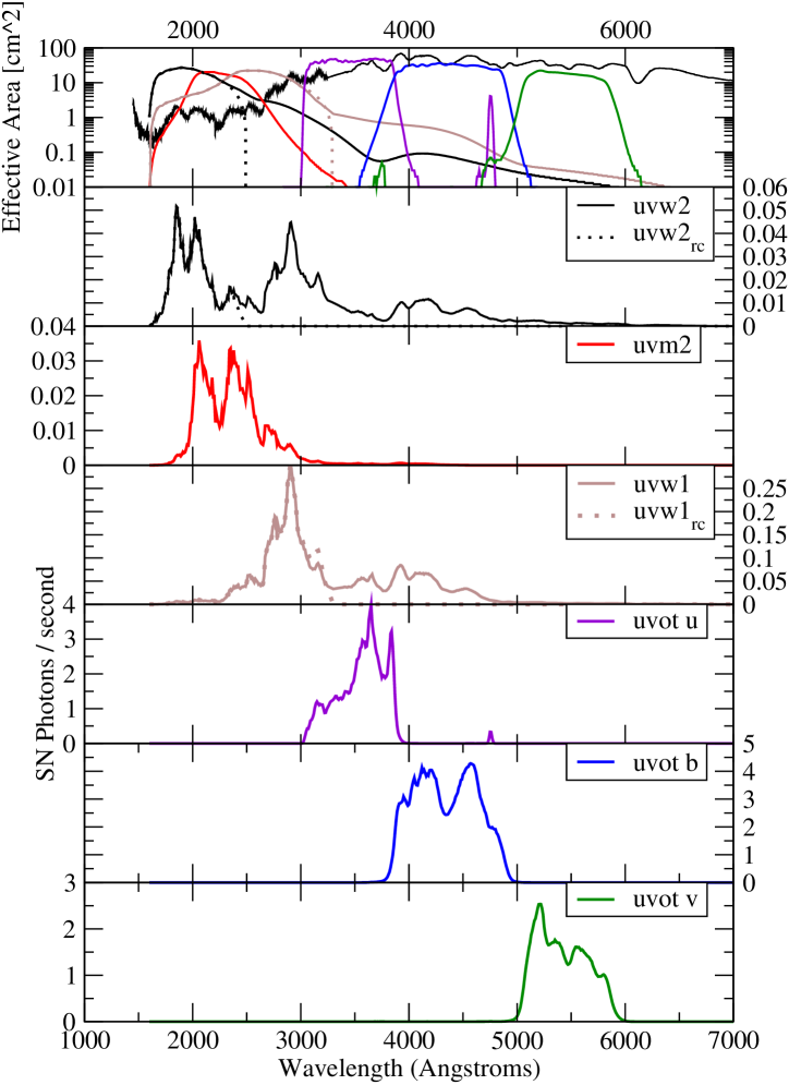
Figure 1: In the top panel, the HST spectrum of SN 1992A (Kirshner et al., 1993) at $\sim 5$ days after maximum brightness is plotted with respect to the six UVOT filters on a logarithmic scale to reveal the structure in the low-flux UV region. The six lower panels show the distribution of photons resulting from the SN 1992A spectrum passing through the six UVOT filters.

While the UV filters have the bulk of their transmission in the near-UV, the red tails of uvw1 and uvw2 combined with the very red SN Ia spectral shape result in a redder distribution of received photons compared to the transmission curves. The uvm2 filter does not have this problem, since its transmission curve is well blocked at longer wavelengths. To visualize the photons UVOT should detect from a SN Ia near maximum light, we multiplied the SN 1992A UV-optical spectrum taken at 5 days after maximum light with HST (Kirshner et al., 1993) with the effective area curves of the UVOT filters (Poole et al., 2008). The resulting photon distributions are displayed in Figure 1. The photon-weighted effective wavelengths (where an equal number of observed photons are longer and shorter than the given wavelength) are listed in Table 1.

In order to better understand the intrinsic UV flux and for comparison with high-redshift observations, it is desirable to estimate the amount of flux coming from the tails and subtract it off. To do this, we first define new filter curves, which we designate uvw2_rc and uvw1_rc (for “red corrected”). These take the latest calibration of the effective areas of the uvw2 and uvw1 filters (Landsman, CALDB document, in preparation). From the uvw2 effective area at 2200 Å (3000 Å for uvw1_rc), the new curves decrease linearly to zero at 2500 Å (3300 Å for uvw1_rc). These curves, and the corresponding photon distribution for the SN 1992A spectrum, are displayed as dashed lines in Figure 1. New zeropoints are determined by passing the spectrum of Vega through the filters and setting its magnitude to zero, thus placing these magnitudes on the Vega system: $ZP_{\rm w2rc}=17.25$ and $ZP_{\rm w1rc}=17.34$ mag, compared to $ZP_{\rm uvw2}=17.35$ and $ZP_{\rm uvw1}=17.49$ mag (Poole et al., 2008). The UVOT magnitudes are determined by $m_{X}=-2.5{\rm log}(\int\lambda/hcf_{\lambda}E_{X,\lambda}d\lambda)+{\rm Zpt}_{X}$. For each SN, we started with one of three spectra: the HST spectrum of SN 1992A from Kirshner et al. (1993), a maximum-light template from Nugent et al. (2002), which incorporated additional IUE UV spectra, or a maximum-light template from Hsiao et al. (2007), which added more HST UV spectra and rest-frame UV spectra from higher redshift SNe. The input spectrum was shifted to the rest frame of the SN and multiplied by a spline function passing through the Vega effective wavelengths of the UVOT filters (uvw2 excluded here) and the ratio of the synthetic to the observed counts in each filter. The uvw2 and $v$ ratios were also used to anchor the spline at the end points of the spectrum, 1600 Å and 8000 Å, respectively. Such a color correction to the spectrum is referred to as “mangling” (Hsiao et al., 2007). This procedure was repeated until the count rates from the mangled spectrum matched the photometry.

To account for the red tails, after the first iteration the uvw2 and uvw1 ratios were scaled by the fraction of the counts in the UV portion (from the previous iteration) in order to better approximate the flux at the reference wavelength. The uvw2 ratio was set to zero when the counts through the tail of the filter already accounted for all of the observed counts. The spectrum was passed through the original and “red corrected” filters (e.g., uvw2 and uvw2_rc), and the magnitude difference was used to transform the observed magnitudes to red tail corrected magnitudes such that uvw2${}_{rc}=$ uvw2$-$rc_w2. This was repeated twenty times for each of the three template spectra, each time randomly offsetting the peak magnitudes consistent with the photometric errors and repeating the mangling and synthetic photometry. The mean and standard deviation were taken to be the correction and its corresponding error. This procedure is not unlike the S-corrections used to correct observations to a standard filter set from filters covering a similar wavelength range but with transmission varying from the standard filter set. In this case the two filters are by definition identical everywhere except at the long-wavelength tail.

The fraction of the estimated counts in each “red-corrected filter” to that of the original filter, and the correction in magnitudes, is listed in Table 3. For uvw1_rc this fraction varies from 0.68 down to 0.29, corresponding to a change in magnitudes (including the different zeropoint) of 0.22 to 0.82 mag. For uvw2_rc the largest fraction is 0.45, corresponding to a magnitude difference of 0.63. Several have essentially no flux in the uvw2_rc filter, with the magnitude of the fraction and correction being largely dependent on how much the iterative mangling depressed the UV portion before the iterations stopped. While this could signify extreme variations in the UV flux, it is more likely indicative of less extreme, but nonetheless very significant, spectral variations in the UV that are not well replicated by mangling the available spectral templates. The shape of these variations can be explored through theoretical modeling (Höflich et al., 1996; Lentz et al., 2000; Sauer et al., 2008) or through additional UV spectra, such as those obtainable with the Cosmic Origins Spectrograph (COS) on the refurbished HST. Recent theoretical modeling does indicate that changes in metallicity have the largest effect in this wavelength region (Sauer et al., 2008), and comparisons with the growing Swift SN sample should put observational constraints on the metallicity range of the observed SNe. Since the correction factors for uvw2_rc are large and uncertain, we will exclude them from our analysis of absolute magnitudes.

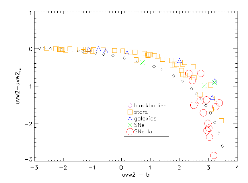
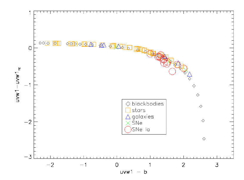
Figure 2: Red-tail corrections for the uvw2 and uvw1 filters plotted with respect to the uvw2$-b$ and uvw1$-b$ colors for a variety of object classes.

For comparison with our SN Ia corrections, and for more general use, similar correction factors were also computed for a large sample of spectra, including stars, galaxies, blackbodies, and other SNe. These are detailed in Appendix A. Figure 2 shows the correction factors as a function of the UV$-b$ colors along with the sample of SNe Ia studied here. The correction factors for a subsample of these are tabulated in Appendix A. Especially for uvw2, the red-tail correction is not a monotonic function of a single color, but different sources of the same color have corrections differing by up to half a magnitude at uvw2$-b\approx 2$. Beyond that, the corrections are too steep to be reliable, but the UV would account for less than 10% of the detected counts anyway. For objects whose general classification is known, the red correction can be determined using the observed UV magnitude and an optical magnitude (which could be obtained from the ground). Otherwise, multiple colors are likely necessary to accurately determine the correction factors in the absence of a suitable template spectrum.

Returning to the SN corrections, the SN Ia colors and calculated corrections place them roughly on the track of the blackbody and stellar spectra. The uvw2_rc corrections are also broadly consistent with low-temperature blackbodies and late-type stellar spectra, but on the steep dropoff where small changes in color correspond to large corrections. This makes the corrections highly uncertain, as differences in the UV spectral shape or errors in the photometry can easily result in an incorrect estimate of the UV flux. Thus, the uvw2 filter will be excluded from this analysis pending further study.

2.3 K-corrections

Despite the low redshift range of our sample, K-corrections (Oke & Sandage, 1968) are non-negligible due to the sharp drop in the SN flux at shorter wavelengths. Thus, even a small shift of the spectrum to longer wavelengths results in less flux being transmitted through the UV filters. To estimate the effect of the K-correction, we have used the template UV spectra mangled to match the observed photometry as described in §2.2. The mangled spectrum was then deredshifted by the host-galaxy redshift, and the synthetic photometry was repeated. The K-correction was then the difference between the observed magnitude of the redshifted spectrum and the observed magnitude of the rest-frame spectrum plus the flux-dilution factor $2.5{\rm log}(1+z)$ (Oke & Sandage, 1968).

The derived K-corrections for each SN are listed in Table 4. The K-corrections in $b$ and $v$ are small, as previously determined by Hamuy et al. (1993); Nugent et al. (2002), but are larger in the UV (see Jha et al., 2006 for a discussion of ground-based $U$-band K-corrections). Uncertainties were estimated from the difference in the K-corrections after offsetting the observed photometry by the photometric errors and repeating the mangling and determination of K-corrections.

More multi-epoch UV spectra of a range of SNe Ia are needed to better understand the UV photometry (including K-corrections) and how much the spectra vary with time and among objects. Spectral differences between SNe may have different effects than accounted for by the mangling, particularly for the SN 1991T and SN 1991bg subtypes. The bulk differences, however, are taken care of by the mangling, and the differences in the red-tail and K-corrections between the SN 1992A spectrum, the Hsiao et al. (2007) and Nugent et al. (2002) templates, and even a flat spectrum after mangling are small in the filters considered. Only uvw2 shows significant differences due to the lack of a reliable flux point at shorter wavelengths.

2.4 Correcting for Extinction

The extinction to a SN has multiple components, as light from the SN can be extinguished by dust surrounding the progenitor, in the host galaxy, in between galaxies, and in the Milky Way. The latter is easy to estimate: we can simply use the reddening maps of Schlegel et al. (1998), and apply a Cardelli et al. (1989) extinction law with $R_{V}=3.1$, corresponding to the average value in the MW. This provides a lower limit to the amount of attenuation undergone by the SN. Estimating the amount of extinction from the other sources, and thus the total line-of-sight extinction, is more difficult.

To estimate the total reddening, we can take advantage of the fact that most SNe Ia have similar post-maximum color evolution in the optical and peak optical colors related to their $\Delta m_{15}(B)$ value. The observed colors can therefore be compared to the expected colors to produce an estimate of the reddening. Table 5 lists three different estimates of this reddening, one based on the color at peak brightness (Phillips et al., 1999; Garnavich et al., 2004), one using the supernova color 30 to 60 days after maximum light (Lira, 1995; Phillips et al., 1999), and two derived from the updated version of the multi-color light-curve shape method (MLCS2k2; Riess et al., 1996a; Jha et al., 2007; Hicken et al., 2009a). For MLCS2k2 we use the values of Hicken et al. (2009a) derived using the MW value of $R_{V}=3.1$ as well as the $R_{V}=1.7$ value which they find gives the best results; these are referred to hereafter as MLCS31 and MLCS17, respectively. In the final analysis, we first adopt the appropriate MLCS2k2 reddening if available, because it considers the colors at all epochs. Otherwise, we use the average of the reddening values determined from the tail and peak colors if available, or just the peak reddening. From the total reddening toward the SN determined by the SN colors with the above methods, the contribution from the MW along the line of sight in the Schlegel et al. (1998) reddening maps is subtracted, and the rest is considered together as the host-galaxy reddening. The reddening from the MW and host-galaxy (determined with different methods) are listed in Table 5.

The Phillips et al. (1999) color relation only applies to the range $0.9<$$\Delta m_{15}(B)$$<1.6$ mag, so for the rapidly declining SNe 2005ke and 2007on ($\Delta m_{15}(B)$ equal to 1.77 and 1.89 mag, respectively) we use the relationship of Garnavich et al. (2004). Both of these SNe, however, appear to have peculiar colors. SN 2005ke is very red at peak, which could be interpreted as a significant reddening of $E(B-V)\approx 0.4$ mag, but the later tail colors and MLCS2k2 fitting (see below) imply a very small host-galaxy reddening, and no interstellar absorption from the host is detectable in high-resolution spectra (Foley 2008, private communication). SN 2007on appears very blue at peak, which results in a negative extinction correction when compared with the peak or tail colors for SNe of similar decay rates; hence, we set the host reddening to be equal to zero. The optical decay rate is also affected by reddening (Phillips et al., 1999), so wherever we use $\Delta m_{15}(B)$, the corrected decay rate $\Delta m_{15}(B)$_true is implied (though this affects the SNe in our sample by at most 0.05 mag).

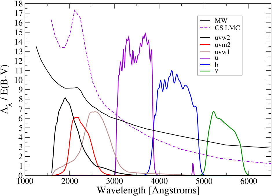
Figure 3: The ratio of selective to total extinction for the MW (Cardelli et al., 1989) and CSLMC (Goobar, 2008) extinction laws plotted as a function of wavelength with the UVOT effective area curves.

The next step is to convert from the $E(B-V)$ reddening to the extinction in each filter. The wavelength dependence of the extinction curves toward SNe is not completely understood, though several well-studied, highly extinguished SNe Ia have been found to have extinction differing from that in the MW (e.g., Elias-Rosa et al., 2006; Wang et al., 2008), and many samples have shown SNe to have systematically lower values of $R_{V}$ than the canonical MW value of 3.1 (e.g., Riess et al., 1996b; Jha et al., 2007; Hicken et al., 2009b; Nobili & Goobar, 2008; Kessler et al., 2009; Folatelli et al., 2010). Whether the UV extinction follows the Cardelli et al. (1989) parameterization according to $R_{V}$ is also uncertain, and the intrinsic reddening law of circumstellar material might be modified by geometric effects (Wang, 2005; Goobar, 2008). For this study we will calculate the host extinction using the $R_{V}=3.1$ extinction law of Cardelli et al. (1989) corresponding to that of the MW (and hereafter designated as MW), and the circumstellar LMC law of Goobar (2008) (hereafter referred to as CSLMC)extended into the UV (Goobar 2010, private communication). The ratios of total to selective extinction for these curves are plotted in Figure 3. In particular, we point out that while the CSLMC ratio is smaller in the optical, consistent with that found in optical studies, the curves cross over in the $u$ band and are much larger in the UV. The true extinction may not correspond to either of these laws, as grain size and distribution may effect the strength of the mid-UV bump and the far-UV rise, and the total extinction may be the sum of components with differing wavelength dependence. It is clear, however, that the UV region is a very sensitive probe of these effects, and future work will include folding these UV data into a multi-wavelength study of extinction. M10 explores a color relation that might be employed to study UV extinction.

To study the effect of extinction in each filter for a SN spectrum, we took the HST UV-optical spectrum of SN 1992A (Kirshner et al., 1993) and extinguished it with the MW extinction law and differing amounts of $E(B-V)$ reddening. We calculated the effective extinction in each UVOT filter by comparing synthetic photometry in the reddened and unreddened spectra. The same was done with the Goobar (2008) CSLMC extinction law. This method is preferred to using a single wavelength (e.g., central, peak, or effective wavelength) to represent the entire filter, since that wavelength is not necessarily representative of the integrated photon distribution.

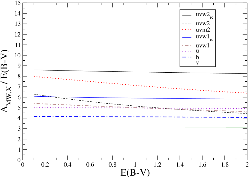
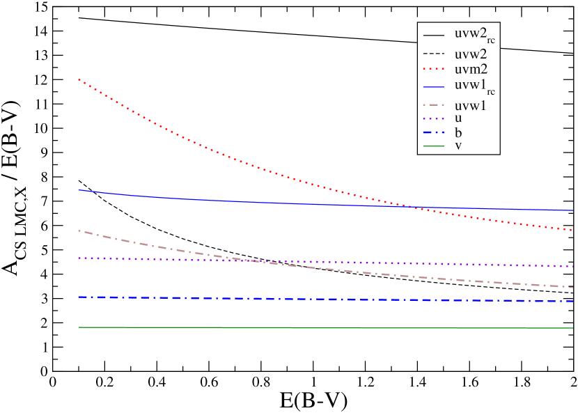
Figure 4: $A_{X}$ divided by $E(B-V)$ as a function of $E(B-V)$ for the six UVOT filters. The MW values are plotted in the left panel and the CSLMC in the right.

For a general understanding of the behavior of the extinction laws, we followed the above steps for a range of $E(B-V)$ values and fit it with an analytic function. Usually, the total extinction through a given filter, $A_{X}$, is related to the differential extinction in a linear fashion, $A_{X}=R_{X}E(B-V)$. Indeed, this is the case for the UVOT $u$, $b$, and $v$ filters, all the way through $E(B-V)=2$ mag. However, as Figure 4 illustrates by plotting $A_{X}/E(B-V)$, the relationship for the UVOT UV filters is highly nonlinear. For both extinction curves, the coefficients for a quadratic fit for $A_{\lambda}$ in terms of $E(B-V)$, such that $A_{\lambda}=R_{1,\lambda}E(B-V)+R_{2,\lambda}E(B-V)^{2}$, are given in Table 1. As evidenced by those coefficients and Figure 4, the quadratic term is unnecessary in the optical but important in the UV. This can be understood in terms of the flux distribution: because dust preferentially extinguishes bluer photons, the effective wavelength of the UVOT broad-band filters becomes redder as the extinction increases. However, this dependence on the spectral shape also means that the extinction coefficients vary with the significantly different colors of the SNe.

To account for both of these effects, extinction coefficients were determined for each SN individually as part of the mangling described above. The observer-frame mangled spectrum was first dereddened by the $R_{V}=3.1$ MW law based on the Schlegel et al. (1998) reddening, and extinction coefficients were determined such that $R_{X}=A_{X}/E(B-V)$. While the effect of MW reddening will change with redshift, in particular as the 2200 Å bump moves in relation to the broad emission and absorption features in the UV spectrum of the SN, the differences are dominated by the varying spectral shapes of the SNe. These are tabulated in Table 6. $R_{X}$ values for a variety of sources are tabulated in Appendix B, and the coefficients for the SNe are consistent with those of other sources with similar colors. After this the spectrum was deredshifted to the SN host frame, and dereddened based on the estimated host $E(B-V)$ together with the $R_{V}=3.1$ MW law and the CSLMC law, and host extinction coefficients determined as above.

2.5 Determining the Distances

Five of our SN host galaxies have independent distance estimates or are in groups whose distances are known from various techniques. NGC 524 (host galaxy of SN 2008Q), NGC 1404 (host galaxy of SN 2007on), the Fornax Cluster (host to SN 2005ke in NGC 1371), and the Hydra Cluster (host to SN 2007cv in NGC 3311) all have distances from the surface brightness fluctuation (SBF) method (Jensen et al., 2003; Tonry et al., 2001; Mieske et al., 2005). These were all placed on the same absolute scale (based on the (Freedman et al., 2001) measurement of the Hubble constant) by adjusting the Tonry et al. (2001) measurements by 0.16 mag, to match the IR-based zeropoint of Jensen et al. (2003). Additionally, SN 2005am (in NGC 2811) and SN 2005df (in NGC 1559) have distance moduli from the luminosity vs. line width (Tully-Fisher) relation, though we do not use the measurement for NGC 2811 because of its large (0.8 mag) uncertainty (Tully et al., 1992). The adopted distances are listed in Table The Absolute Magnitudes of Type Ia Supernovae in the Ultraviolet.

For the remaining SNe, we adopted a distance based on the recession velocities of their host galaxies, a model for the local velocity flow (Mould et al., 2000), and $H_{0}=72$ km s^-1 Mpc^-1 (Freedman et al., 2001). We ignore the stated 8 km s^-1 Mpc^-1 uncertainty in the Hubble constant since an error would cause a shift in the absolute magnitudes but not affect the scatter, which is our primary measure of the standardizability of SNe Ia in the UV. The Hubble-flow distances for all of the SNe are listed in Table The Absolute Magnitudes of Type Ia Supernovae in the Ultraviolet, along with an uncertainty which is based on a possible peculiar motion of 150 km s^-1, but in the subsequent analysis we use only the Hubble-flow distances for the SNe which do not have an independent distance measurement.

Finally, we check our distance estimates by exploiting the fact that SNe Ia are standardizable candles in the optical. Table The Absolute Magnitudes of Type Ia Supernovae in the Ultraviolet gives the distance measured using MLCS2k2 with both $R_{V}=3.1$ and 1.7 (scaled to the same H${}_{0}=72$ scale used above. Eight of these SN distances were reported by Hicken et al. (2009a) and an MLCS2k2 distance with $R_{V}=3.1$ for SN 2005df was reported by M10. Of the nine SNe with MLCS2k2 distances, six of the SN distances are within $1\sigma$ of the adopted distance, and three are about $2\sigma$ away (with the uncertainties added in quadrature).

We also used NED and HyperLeda (Paturel et al., 2003) to find the Hubble morphological type (translated from the de Vaucouleurs scale when necessary; de Vaucouleurs et al., 1991). The classifications and individual references are given in Table The Absolute Magnitudes of Type Ia Supernovae in the Ultraviolet. The majority of the SNe in our sample are found in late-type galaxies. Of those in early-type galaxies, the hosts of SNe 2005cf, 2006dm, and 2006ej are distorted by interactions with other galaxies, so the progenitor could have arisen from relatively recent star formation. A larger sample of SNe arising from older stellar populations is needed to compare UV properties from different environments.

3 Results

3.1 Peak Pseudocolors vs. Reddening

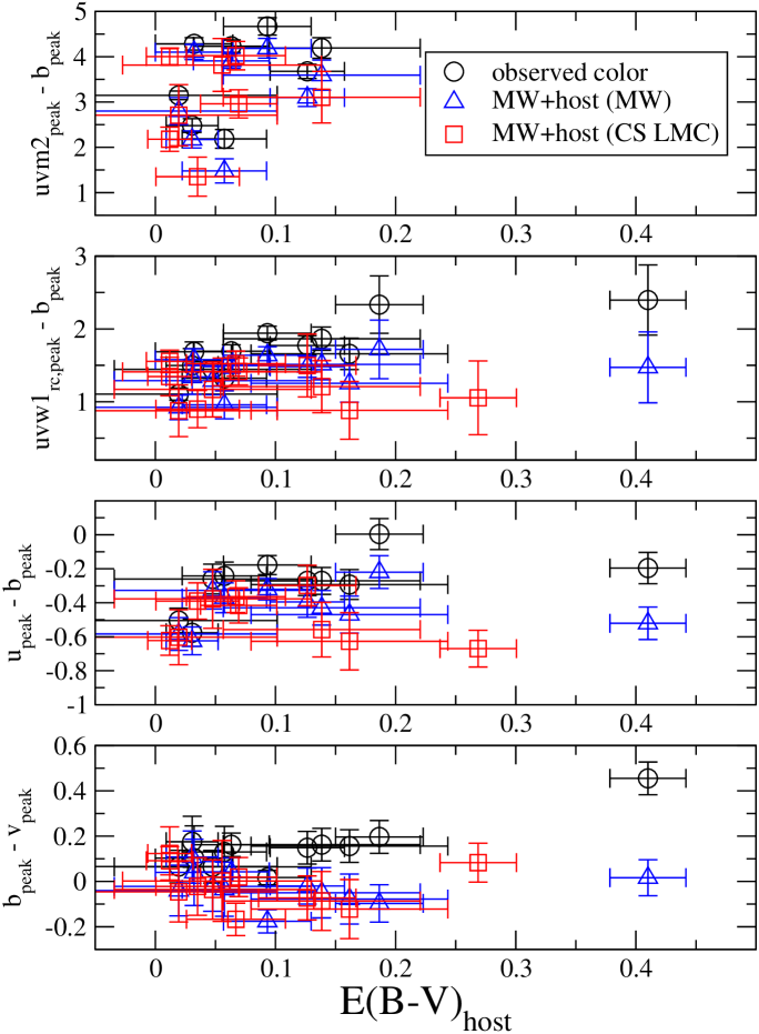
Figure 5: UV$-b$ colors of the SNe Ia with $\Delta m_{15}(B)<1.6$ mag without extinction correction and after correction for Galactic and host-galaxy reddening (corrected with the MW and CSLMC extinction laws). For the observed colors, the abscissa corresponds to the MLCS31 host reddening. Since the MLCS17 model gives a different value for the host reddening, the same SNe do not always line up vertically. There does not appear to be any significant difference in the extinction-corrected colors, though the sample is small and the SNe in our sample with the highest reddening values also have the lowest values of $\Delta m_{15}(B)$.

We first examine the peak colors to verify that our extinction correction does not leave or create any bias in the colors. Figure 5 plots the difference between the maximum UV magnitude of the normal SN and its maximum $b$ magnitude, corrected for reddening based on the Galactic and adopted host-galaxy reddening and the MW and CSLMC extinction laws, as a function of the host reddening. These “pseudocolors” are relatively constant with $R(B-V)$, so no reddening law is clearly better. The two SNe with the highest host reddening are also the SNe with the broadest optical light curves of the sample, and neither are detected in the uvm2, so it would be difficult to draw strong conclusions based on them. A similar exercise done with a larger sample of moderately extinguished SNe is needed to determine if one of the reddening laws is superior. Deeper observations in the uvm2 filter are also required to get a better handle on the UV extinction, where the differences are largest, without the uncertainties of the red-tail correction.

The uncertainty in the reddening also propagates to a higher uncertainty in the extinction because of the large extinction coefficients in the UV. For example, a modest change in $E(B-V)$ of 0.05 mag (the dispersion in the Lira relation; Phillips et al., 1999) shifts $A_{m2}$ by $\sim 0.4$–0.7 mag. However, this large lever arm can provide useful constraints on the measurement of interstellar reddening, just as expanding the wavelength range of the measurements in the other direction to the near-IR has already increased the accuracy of extinction corrections (Elias-Rosa et al., 2006; Krisciunas et al., 2007; Mandel et al., 2009).

3.2 Peak Pseudocolors vs. $\Delta m_{15}(B)$

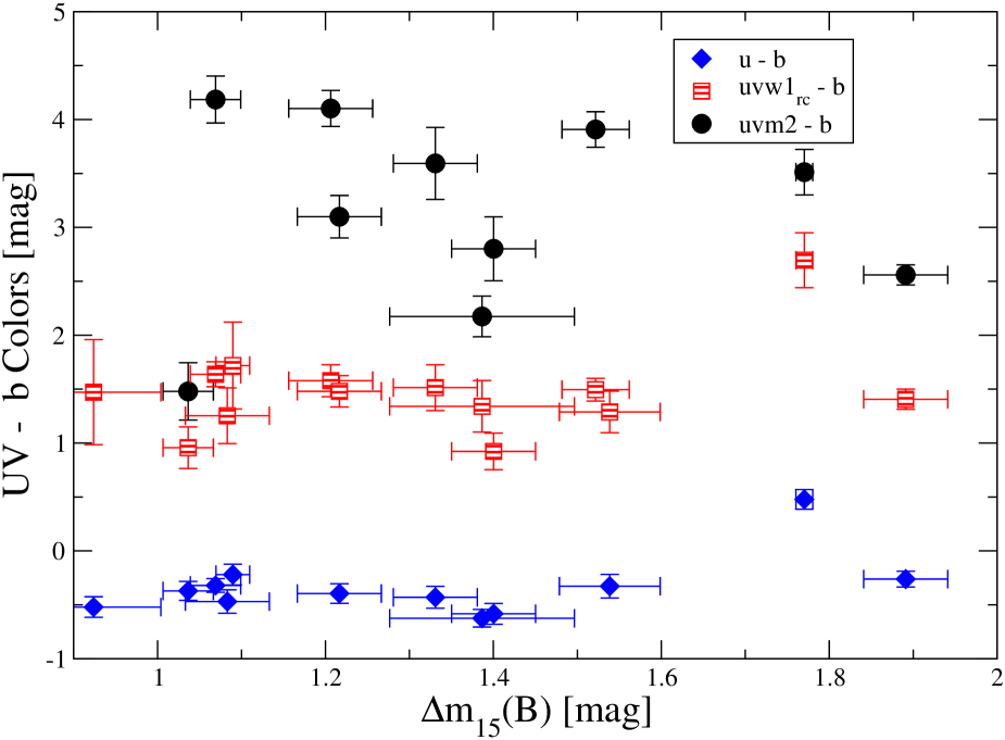
Figure 6: Peak UV$-b$ pseudocolors plotted with respect to their optical decay rate $\Delta m_{15}(B)$. The colors have been corrected for Galactic and host reddening using the MW extinction law. SN 2005ke, at $\Delta m_{15}(B)=1.77$ mag, is much redder than the other SNe in $u-b$ and uvw1${}_{rc}-b$, but not so different in uvm2$-b$. The same behavior is seen when the host reddening is corrected with the CSLMC law.

Without the added uncertainties from distances, we can take a first look at how standard the UV peak magnitudes are by comparing them with the standardizable optical peak magnitudes. Figure 6 shows the UV-optical pseudocolors of each supernova at maximum, plotted against optical decay rate, $\Delta m_{15}(B)$. The colors are relatively flat with respect to $\Delta m_{15}(B)$. SN 2005ke, at $\Delta m_{15}(B)=1.77$ mag, appears as a red outlier in $u-b$ and uvw1${}_{rc}-b$, but not in uvm2$-b$. Note that our $u-b$ plot does not show the reddening trend present in ground-based $U-B$ data (Jha et al., 2006). However, considering that the UVOT $u$-band filter is bluer than Johnson $U$, and that the reddening trend seen by Jha et al. (2006) reverses at shorter wavelengths (Foley et al., 2008b), this result is reasonable.

Average reddening-corrected colors for our SNe with $\Delta m_{15}(B)<1.6$ mag are listed in Table 8. The colors corrected with the CSLMC law are up to 0.15 mag bluer due to the steeper correction, but the differences in the scatter are 0.03 mag or less. In the following we compare the scatter in different colors using the MW-corrected values but the trend is the same for the CSLMC law. Compared to the 0.07 mag scatter in the $b-v$ colors, the scatter increases modestly in the $u-b$ and uvw1${}_{rc}-b$ bands to 0.13 and 0.25 mag respectively. The uvm2$-b$ colors scatter by 0.97 mag and show no correlation with $\Delta m_{15}(B)$, evidence of very different behavior in the mid-UV which does not follow the one-parameter family that dominates the optical luminosity-width relation.

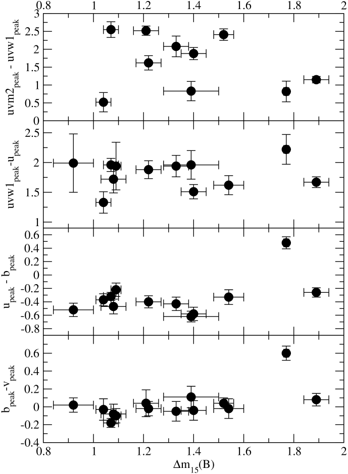
Figure 7: Various extinction corrected colors plotted with respect to the optical decay rate $\Delta m_{15}(B)$. While many subluminous SNe Ia can be identified in the optical by their very red colors, SN 2007on does not follow this trend, and the UV colors of both SNe 2005ke (which is very red in $b-v$ and $u-b$) and 2007on are similar to those of normal SNe Ia. The same behavior is seen when the host reddening is corrected with the CSLMC law.

Considering colors of neighboring bands gives one a crude view of the spectral shape and variability between objects. These colors are displayed in Figure 7. We see that uvw1${}_{rc}-u$ has a modestly larger scatter as does $u-b$, but that of uvm2$-$uvw1_rc is much larger. While the differences are very small in the 4000–6000 Å ($bv$) regions, they become modestly larger over the intervals 3000–5000 Å and 2500–4000 Å. The region shortward of $\sim 2500$ Å is found to be much more diverse. Also of note is that while SN 2005ke is red in $b-v$, $u-b$, and uvw1${}_{rc}-u$, it appears normal in uvm2$-$uvw1_rc, suggesting that the strong spectral differences do not extend as far in the UV. In a comparison of the near-UV spectra of high-redshift SNe Ia, both Ellis et al. (2008) and Foley et al. (2008a) found an increase in the spectral diversity shortward of $\sim 3700$ Å. Computing colors for those spectra in the UVOT filters would allow the best comparison of the dispersion and the UV shape (Sullivan et al., 2009) at low and high redshifts.

3.3 Absolute Magnitudes

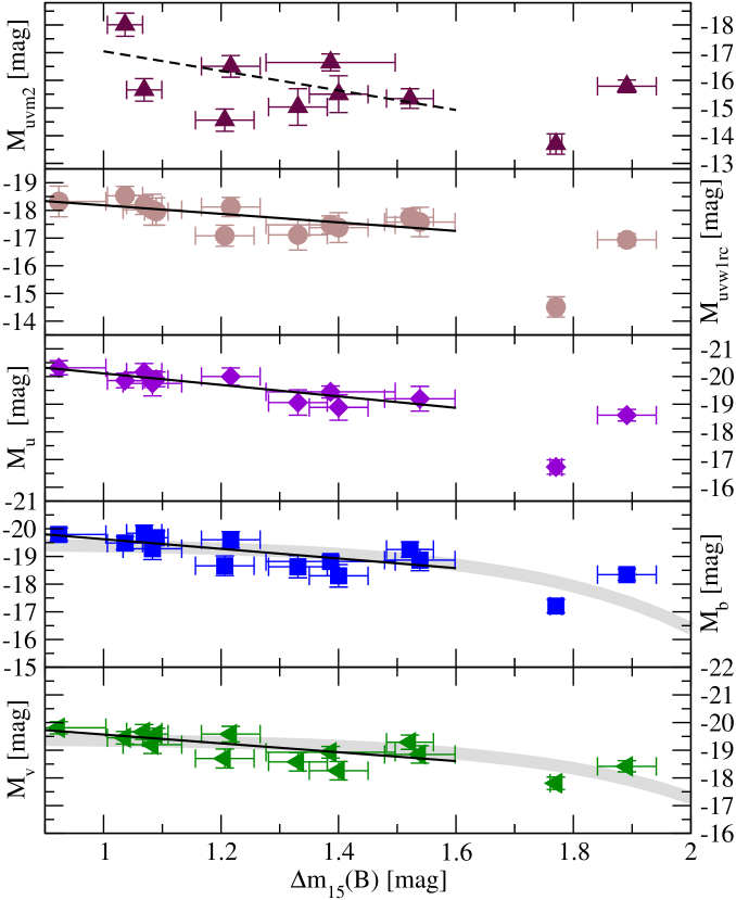
Figure 8: UV and optical absolute magnitudes, calibrated with independent or Hubble-flow distances, plotted with respect to their optical decay rate $\Delta m_{15}(B)$. The host-galaxy reddening was corrected using the MW law. Similar to the optical, the absolute magnitudes in the $u$ and uvw1 bands become slightly fainter with $\Delta m_{15}(B)$ for the SNe with $0.9\leq\Delta m_{15}(B)\leq 1.6$ mag. Black lines show a fit to the absolute magnitudes with respect to $\Delta m_{15}(B)$. The absolute magnitudes in the uvm2 filter show considerably more scatter and are only poorly fit with $\Delta m_{15}(B)$. SN 2005ke is even fainter in the optical and near-UV filters than one would expect based on its $\Delta m_{15}(B)$, but SN 2007on is brighter. The grey lines represent the Garnavich et al. (2004) absolute magnitudes in $B$ and $V$, with the dispersion of 0.2 mag represented by the width of the line.

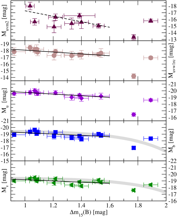
Figure 9: UV and optical absolute magnitudes, calibrated with independent or Hubble-flow distances, plotted with respect to their optical decay rate $\Delta m_{15}(B)$. The host-galaxy reddening was corrected using the CSLMC law. The plot is very similar to Figure 8, with the moderately extinguished SN 2007S on the left side being the only one that moves significantly compared to the others.

Tables 9 and 10 list the absolute magnitudes for all of our SNe computed using the apparent magnitudes of Table The Absolute Magnitudes of Type Ia Supernovae in the Ultraviolet, the red-tail correction for uvw1 of Table 3, the K-corrections of Table 4, the MW and host-galaxy reddenings (corrected with the MW and CSLMC extinction laws) of Table 5, and the independent or Hubble-flow distance moduli of Table The Absolute Magnitudes of Type Ia Supernovae in the Ultraviolet. These absolute magnitudes are plotted in Figures 8 and 9 with respect to the extinction-corrected optical decay rate $\Delta m_{15}(B)$ from either UVOT or ground-based observations (also listed in Tables 9 and 10 for easier identification of the SNe).

The absolute magnitudes in the optical and UV, calculated with either the MW or CSLMC extinction law, show similar behavior for low values of $\Delta m_{15}(B)$. Within the range $0.9<\Delta m_{15}(B)<1.6$ mag, the $v$, $b$, $u$, and uvw1_rc absolute magnitudes scatter about the average by $\sim 0.4$–0.5 mag (Table 11). The uvm2 absolute magnitudes have a larger dispersion of $\sim 1$ mag. Fitting the absolute magnitudes of the SNe with respect to $\Delta m_{15}(B)$ within the range $0.9<\Delta m_{15}(B)<1.6$ mag, we find a slightly steeper slope at shorter wavelengths, though the scatter in uvm2 is especially large and the fit not well constrained. The scatter about the linear fit decreases to $\sim 0.3$–0.4 mag in the $v$, $b$, $u$, and uvw1_rc filters. To estimate the intrinsic scatter along such a linear relation, we tested how much scatter needed to be added in quadrature to the estimated uncertainties in order for the reduced $\chi^{2}$ to be near unity. No intrinsic scatter is required for the $v$, $b$, $u$, and uvw1_rc filters — the reduced $\chi^{2}$ values are much less than unity, indicating that the observed scatter is consistent with the estimated uncertainties and that those uncertainties might be overestimated. So while the $b$ and $v$ scatter apparent in Figures 8 and 9 is larger than that found for most other samples of SNe Ia (typically $\sim 0.2$ mag; Hamuy et al., 1996a; Phillips et al., 1999; Altavilla et al., 2004; Garnavich et al., 2004), it is consistent with our estimated uncertainties.

In the uvm2, however, the absolute magnitudes do require an additional scatter to have an acceptable reduced $\chi^{2}$. The amount of intrinsic dispersion required is 0.8 mag for the MW extinction law and 0.4 mag for the CSLMC law. This reduction is likely due to the larger uncertainties in the extinction due to the much larger value of $R_{\rm uvm2}$. That intrinsic scatter is required above the observational errors is significant, considering that the optical absolute magnitudes have intrinsic scatter masked by our errors.

Since a significant fraction of the scatter in the optical and near-UV could come from the Hubble-flow distances, the absolute magnitudes were also computed using the SN-derived MLCS31 (MLCS17) distances. For the subsample of normal SNe with MLCS31 (MLCS17) distances, this drops the scatter in the absolute magnitudes in $v$, $b$, $u$, and uvw1_rc from 0.18, 0.23, 0.16, and 0.21 (0.20, 0.28, 0.19, and 0.25) mag to 0.15, 0.15, 0.22, and 0.22 (0.11, 0.13, 0.22, and 0.22) mag, respectively. The scatter drops in the optical, as is expected for a distance calculation based on the optical magnitudes, but the near-UV scatter is not changed significantly. The uvm2 scatter actually increases slightly from 0.88 to 1.00 (0.90 to 0.99) mag, reinforcing the conclusion that most of the scatter in uvm2 is intrinsic.

Our two SNe having high values of $\Delta m_{15}(B)$ are much harder to interpret. SNe 2005ke is significantly fainter than the rest of the sample in the UV filters as well as in the optical, where it is fainter than other subluminous SNe with the same decay rate, represented by the Garnavich et al. (2004) relation plotted in grey in Figures 8 and 9. Conversely, SN 2007on is brighter than the Garnavich et al. (2004) relation and in the UV has an absolute magnitude comparable to that of the normal SNe Ia. Phillips (2009, private communication) reports that spectroscopically SN 2007on appears more similar to SNe having $\Delta m_{15}(B)$ $\approx 1.6$ mag, suggesting that $\Delta m_{15}(B)$ is not a good discriminator for the most rapidly declining SNe. Recent work by Krisciunas et al. (2009) shows that SNe Ia may exhibit a bimodal distribution in the near-IR and optical absolute magnitudes in this range of $\Delta m_{15}(B)$, hence similar differences in the UV should not be surprising.

3.4 Search for Photometric UV Luminosity Indicators

The optical light of the highest-redshift SNe will be hard to observe, so it would be valuable to have a distance-independent luminosity indicator observable in the UV data to calibrate the magnitudes either as a proxy for $\Delta m_{15}(B)$ or as a separate luminosity indicator. Unfortunately, no such parameter has yet been found in our photometry.

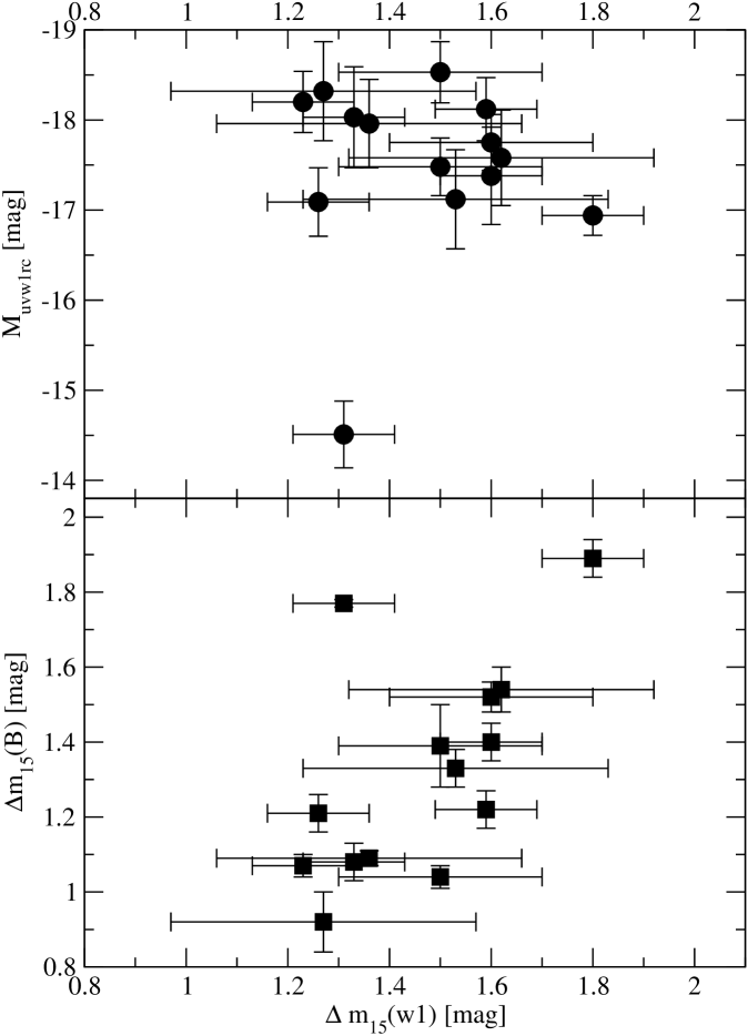
Figure 10: The uvw1 absolute magnitude and the optical decay rate $\Delta m_{15}(B)$ are plotted with respect to the uvw1 decay rate. The uvw1 absolute magnitudes have been corrected using the MW extinction law, but the same behavior is seen with the CSLMC law. While the uvw1_rc absolute magnitudes and $\Delta m_{15}(uvw1)$ both correlate weakly with $\Delta m_{15}(B)$, there is no strong correlation between the absolute magnitudes and $\Delta m_{15}(uvw1)$, which occupies a narrower range than its optical counterpart.

M10 parameterized the shapes of UV light curves in a manner similar to that of Phillips (1993), measuring the amount a supernova fades in the first 15 days after maximum light. However, as was noticed after the first five SNe Ia observed with Swift (Immler et al., 2006), the early uvw1 light curves of all our SNe Ia are similar. As shown in Figure 10, the range of $\Delta m_{15}({\rm uvw1})$ is only $\sim 0.5$ mag (compared to the $\sim 1$ mag difference between slow and fast decliners in the optical). Moreover, within that small range, there is no correlation between $\Delta m_{15}({\rm uvw1})$ and $\Delta m_{15}(B)$ or the uvw1_rc absolute magnitude. The range of decay rates is larger in the uvm2 band, but again, the scatter in the absolute magnitude vs. optical decay-rate relation is much stronger than any systematic trend. M10 do find a correlation between the optical decay rate and the time that the light curve breaks from its steep to shallow decay, but there is no clear correlation between the time of the break and the UV absolute magnitudes.

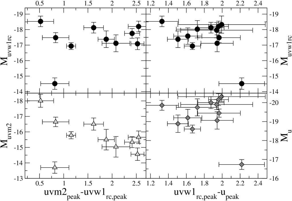
Figure 11: uvm2, uvw1_rc, and $u$ absolute magnitudes are plotted vs. uvm2$-$uvw1_rc and uvw1${}_{rc}-u$ colors. There is no clear correlation except in uvm2, where the absolute magnitudes (with the exception of SN 2005ke) correlate with the colors because of the large dispersion in uvm2 compared to uvw1_rc. The uvw1 absolute magnitudes have been corrected using the MW extinction law, but the same behavior is seen with the CSLMC law.

Correlations between the absolute magnitudes and peak colors would be most useful, since following a UV light curve as it fades would be increasingly more difficult at higher redshifts. The UV colors in our small sample, however, do not show a strong correlation between the UV colors and $\Delta m_{15}(B)$, displayed in Figure 6. Figure 11 directly compares the UV absolute magnitudes vs. UV colors, which is what would be very useful for measuring distances using only UV observations. There is no clear correlation except in uvm2, where we essentially see the absolute magnitudes correlate with the colors because of the large dispersion in uvm2 compared to uvw1_rc.

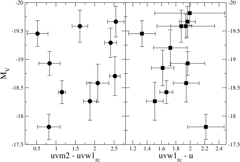
Figure 12: Absolute $V$ magnitudes plotted with respect to the UV colors. No correlation is seen to correspond with the near-UV spectral correlation found by Foley et al. (2008b). The uvw1 absolute magnitudes have been corrected using the MW extinction law, but the same behavior is seen with the CSLMC law.

Foley et al. (2008b) have reported a possible correlation between the peak luminosity of a SN Ia and its spectral slope between 2770 Å and 2900 Å. While most Swift grism spectra do not have sufficiently high signal-to-noise ratio to measure this ratio (Bufano et al., 2009), Foley et al. (2008b) suggested that UVOT colors might exhibit the same trend, but Figure 12 shows that the correlation is not seen in the photometric colors of the larger bandpasses. However, as the scatter in our optical absolute magnitudes is consistent with the observational errors, it would be difficult to find a correlation with the intrinsic differences. The broad-band filters may also wash out the spectral features or exaggerate small errors in the extinction.

4 Discussion

The UV absolute magnitudes of this sample of SNe Ia seem to show two distinct types of behavior. At near-UV wavelengths (2500–4000 Å) probed by UVOT uvw1_rc and $u$ and by ground-based $U$ (Jha et al., 2006), the absolute magnitudes show a similar relationship to the optical decay rate $\Delta m_{15}(B)$ as do the optical absolute magnitudes. As shown in Table 11, for this sample the scatter in the absolute magnitudes of SNe Ia at peak is comparable in the near-UV and optical. However, this scatter is higher than that found in the optical for larger samples (typically $\sim 0.2$ mag; Hamuy et al., 1996a; Phillips et al., 1999; Altavilla et al., 2004; Garnavich et al., 2004), and the UV scatter could be significantly higher. If larger samples put tighter limits on the intrinsic dispersion, the near-UV could be useful for measuring luminosity distances. This would be most valuable at higher redshifts where fewer optical bands are available, to put multi-color constraints on the reddening and distance. How useful they could be depends on the intrinsic scatter, which is hard to measure in this sample due to its small size and large observational uncertainties. While larger samples are now available in $U$ (Jha et al., 2006; Hicken et al., 2009a), the space-based UV sample is still relatively small — comparable to the 9 objects used by Phillips (1993) to discover the peak absolute magnitude vs. decline-rate relation. Just as the systematics of optical absolute magnitudes have been refined with larger samples of objects, an increased number of UV measurements is needed to better understand the behavior of SNe in the UV. The origin and wavelength dependence of extinction, and the uncertainty in the red-tail and K-corrections due to intrinsic differences in the UV spectra, are needed to improve the utility of the near-UV SN photometry.

Conversely, the absolute magnitudes in the mid-UV (2000–2500 Å, the UVOT uvm2 band) exhibit a large scatter and therefore are less useful for distance determinations. Studying the cause of that scatter in nearby events, however, should assist us in understanding the SN Ia phenomenon, as well as the effect that different reddening laws or host environments have on distance estimates.

Metallicity differences have been suggested as a possible second parameter in the optical maximum magnitude vs. rate of decline relation (e.g., Mazzali & Podsiadlowski, 2006). A metallicity-dependent component to the absolute magnitudes could result in an evolutionary bias as one observes higher-redshift SNe with likely different metallicities(Podsiadlowski et al., 2006). A concern already for the optical, this could be even more critical in the UV where the metallicity plays a strong role in the reverse-fluorescence emission (Mazzali, 2000; Sauer et al., 2008) as well as in the line blanketing (see Lentz et al., 2000; Dominguez et al., 2001). Moreover, a change in metallicity could also bias SN-based extinction measurements which are calibrated using the $B-V$ color of local objects (Dominguez et al., 2001). A better understanding could be reached through detailed studies of the ages and metallicities of SN host galaxies (Gallagher et al., 2008) observed in the UV, and by a search for correlations of such measures with the UV luminosity and colors (Sauer et al., 2008). If a correlation can be found, then the UV data might provide leverage in probing the metallicity dependence on the optical brightness and its evolution with redshift, thus making SNe Ia even better standardized candles in the optical. There is disagreement as to whether metallicities have already been found to affect optical measurements (Gallagher et al., 2008; Howell et al., 2009).

In general, the measurements of SNe Ia in the UV are hindered by the low UV flux caused by metal line blanketing and extinction, yet the strong sensitivity to these effects makes the UV region important for constraining these parameters. Thus, while rest-frame UV measurements may not be ideal for cosmological distance measurements, the understanding gleaned from UV data of local events will shed light on the important effects of extinction and metallicity and how they might evolve with redshift, thereby improving the reliability of SNe Ia as cosmological standard candles.

Appendix A Red-Tail Corrections for Other Sources

Vega magnitudes in the nominal UVOT filters and our red-tail-corrected uvw2_rc and uvw1_rc were generated for a large sample of different sources. For stars we used the empirical stellar spectra database of Pickles (1998). Most of the Pickles spectra of later type stars (G and beyond) have zero flux in the UV, and those are excluded here. A representative UV-optical galaxy spectrum for the main Hubble types from McCall (2004) was used, together with synthetic spectra of a single burst of star formation viewed at one and fifteen Gyr computed using the model code PÉGASE (Fioc & Rocca-Volmerange, 1997). Blackbody curves corresponding to temperatures ranging from 2,000 to 35,000 K were also used, as were HST UV spectra from a SN of each major type: SNe 1992A (Ia; Kirshner et al., 1993), 1994I (Ic; Jeffery et al., 1994), and 1999em (IIP; Baron et al., 2000). Various UV and UV-optical colors as well as the red-leak correction factors were determined for each spectrum, and these are tabulated for a subset of spectra in Table 12.

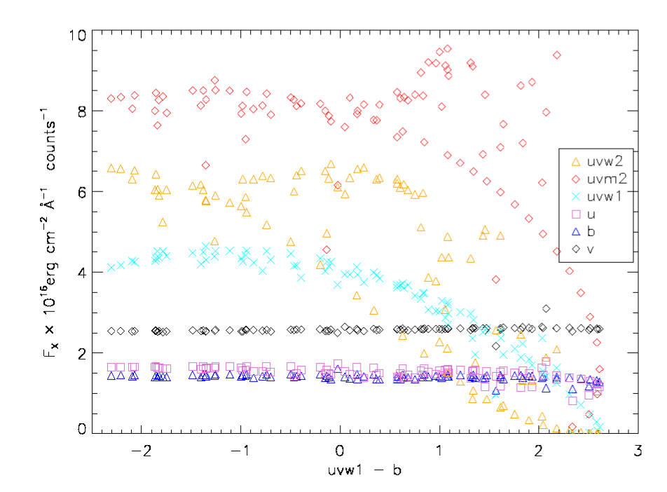
Figure 13: Flux conversion factors for the UVOT filters calculated for a variety of spectra. Multiplying the observed count rate in a given filter by the appropriate conversion factors gives the flux density the template spectrum has at the filter’s effective wavelength for Vega. The factors are fairly constant across different spectral types in the optical for this range of models but vary greatly in the UV.

The shape of the filter curves also strongly affects the calculation of the flux density for different spectral shapes. For comparison of the flux of different objects, we keep the reference wavelength fixed at the effective wavelengths determined for Vega (Poole et al., 2008) rather than allowing them to vary with the spectral shape. For each spectrum and filter, we determine the flux conversion factor by dividing the average flux density in a 50 Å window centered on the reference wavelength by the count rate of the spectrum through that filter. Thus, one multiplies the observed count rate by the conversion factor to get the approximate flux-density value. Poole et al. (2008) presented average flux conversion factors for a set of stellar and gamma-ray burst (power-law) models. Here we expand on this by giving the flux conversion factors individually for the set of spectra in Table 13. In Figure 13 we show the flux conversion factors varying strongly with the UV-optical color. Accounting for this variation is critical for computing the UV flux for red objects, as the average conversion factors assume an average flux distribution, while for red objects the observed counts are heavily biased to the red end of the filter curves.

Appendix B Extinction Coefficients

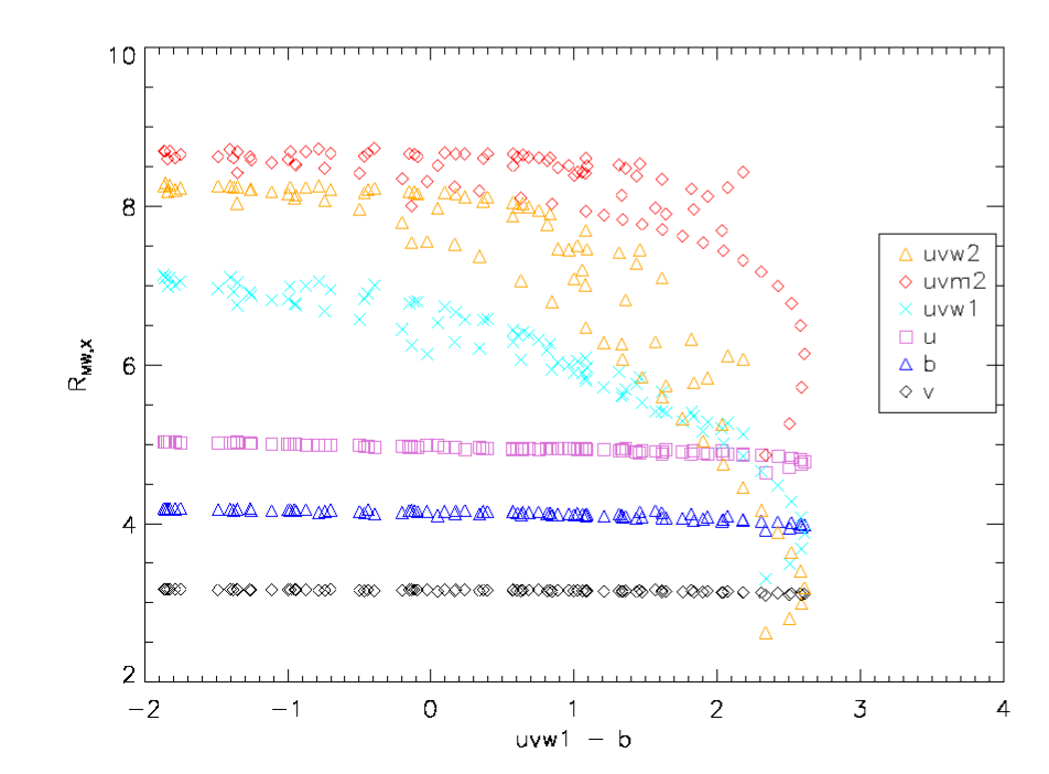
Figure 14: Extinction coefficients for the UVOT filters calculated for a variety of spectra using the Cardelli et al. (1989) MW extinction law and $E(B-V)=0.1$ mag. The uvw1$-b$ color on the abscissa is the unreddened color. The factors are fairly constant in the optical for this range of models but vary greatly in the UV.

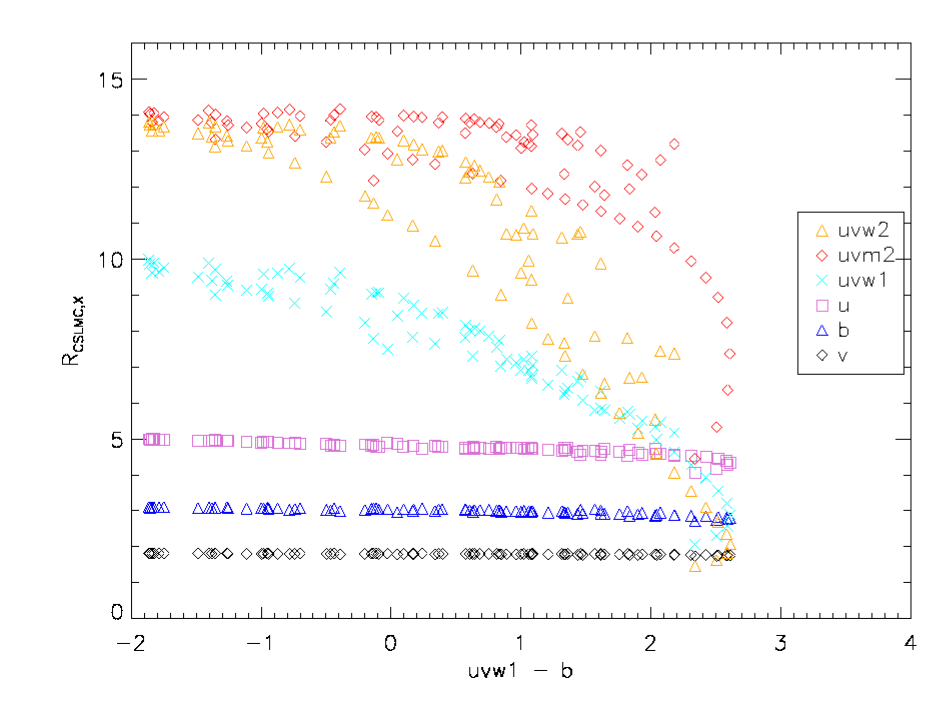
Figure 15: Extinction coefficients for the UVOT filters calculated for a variety of spectra using the Goobar (2008) circumstellar LMC extinction law and $E(B-V)=0.1$ mag. The uvw1$-b$ color on the abscissa is the unreddened color. The factors are fairly constant in the optical for this range of models but vary greatly in the UV.

Extinction coefficients are used to convert a measure of reddening to the total extinction in a given filter X as in $A_{X}=R_{X}\times E(B-V)$. Since the extinction is a function of wavelength and the filters have nonzero width, the effect of the reddening depends on the spectral shape being extinguished. Since in general extinction increases to shorter wavelengths, a blue source is more efficiently extinguished than a red source. Below we extinguish the same set of spectra by the (Cardelli et al., 1989) $R_{V}=3.1$ MW extinction curve or the (Goobar, 2008) circumstellar LMC extinction law for $E(B-V)=0.1$ mag. The magnitude difference between the extinguished and unextinguished spectra gives the extinction in each filter. The coefficients are plotted in Figures 14 and 15 and tabulated in Tables 14 and 15.

Table 1: UVOT Filter Characteristics

Filter	$\lambda_{\rm central}$	FWHM	$\lambda_{\rm eff,Vega}$	$\lambda_{\rm eff,SNIa}$	$R_{\rm MW},1,X$	$R_{\rm MW},2,X$	$R_{\rm CSLMC},1,X$	$R_{\rm CSLMC},2,X$
	(Å)	(Å)	(Å)	(Å)	(mag)	(mag)	(mag)	(mag)
uvw2	1941	556	2030	3064	6.20	-0.95	6.77	-2.07
uvw2rc	1941	556	$\cdots$	2010	8.60	-0.18	14.58	-0.75
uvm2	2248	514	2231	2360	8.01	-0.85	11.33	-3.13
uvw1	2605	653	2634	3050	5.43	-0.41	5.58	-1.17
uvw1rc	2605	653	$\cdots$	2890	6.06	-0.13	7.33	-0.39
$u$	3464	787	3501	3600	4.92	-0.03	4.68	-0.17
$b$	4371	982	4329	4340	4.16	-0.04	3.06	-0.09
$v$	5441	730	5402	5400	3.16	-0.01	1.81	-0.01

Table 2: Apparent Magnitudes at Maximum Light

Name	$\Delta m_{15}(B)$	uvw2	uvm2	uvw1	$u$	$b$	$v$	ref
	(mag)	(mag)	(mag)	(mag)	(mag)	(mag)	(mag)
SN 2005am	1.52 $\pm$ 0.04	16.95 $\pm$ 0.08	18.26 $\pm$ 0.13	15.35 $\pm$ 0.06	$\cdots$	13.90 $\pm$ 0.04	13.75 $\pm$ 0.03	1,2
SN 2005cf	1.07 $\pm$ 0.03	16.83 $\pm$ 0.08	18.32 $\pm$ 0.19	15.11 $\pm$ 0.07	13.41 $\pm$ 0.05	13.54 $\pm$ 0.02	13.53 $\pm$ 0.02	3,3
SN 2005df	1.21 $\pm$ 0.05	15.61 $\pm$ 0.07	16.85 $\pm$ 0.09	13.90 $\pm$ 0.07	$\cdots$	12.50 $\pm$ 0.10	12.40 $\pm$ 0.10	4,4
SN 2005ke	1.77 $\pm$ 0.01	18.41 $\pm$ 0.11	18.87 $\pm$ 0.15	17.09 $\pm$ 0.09	15.52 $\pm$ 0.07	14.92 $\pm$ 0.05	14.22 $\pm$ 0.05	5,U
SN 2006dm	1.54 $\pm$ 0.06	18.93 $\pm$ 0.13	$\cdots$	17.63 $\pm$ 0.09	15.99 $\pm$ 0.07	16.17 $\pm$ 0.05	16.13 $\pm$ 0.05	1,U
SN 2006ej	1.39 $\pm$ 0.11	18.73 $\pm$ 0.13	18.46 $\pm$ 0.14	17.00 $\pm$ 0.08	15.47 $\pm$ 0.06	15.93 $\pm$ 0.05	15.80 $\pm$ 0.10	1,U
SN 2007S	0.92 $\pm$ 0.08	$\cdots$	$\cdots$	17.80 $\pm$ 0.14	15.86 $\pm$ 0.07	15.94 $\pm$ 0.05	15.53 $\pm$ 0.05	U,U
SN 2007af	1.22 $\pm$ 0.05	16.50 $\pm$ 0.09	17.12 $\pm$ 0.15	14.77 $\pm$ 0.07	13.16 $\pm$ 0.07	13.39 $\pm$ 0.05	13.25 $\pm$ 0.05	U,U
SN 2007co	1.09 $\pm$ 0.02	20.11 $\pm$ 0.20	$\cdots$	18.80 $\pm$ 0.15	16.99 $\pm$ 0.07	16.86 $\pm$ 0.05	16.69 $\pm$ 0.05	U,U
SN 2007cq	1.04 $\pm$ 0.03	18.61 $\pm$ 0.13	18.53 $\pm$ 0.19	17.53 $\pm$ 0.11	16.12 $\pm$ 0.06	16.27 $\pm$ 0.05	16.17 $\pm$ 0.10	2,U
SN 2007cv	1.33 $\pm$ 0.05	18.47 $\pm$ 0.13	19.60 $\pm$ 0.22	16.83 $\pm$ 0.09	15.08 $\pm$ 0.06	15.30 $\pm$ 0.05	15.15 $\pm$ 0.05	U,U
SN 2007on	1.89 $\pm$ 0.05	15.65 $\pm$ 0.05	15.78 $\pm$ 0.05	14.36 $\pm$ 0.05	12.93 $\pm$ 0.05	13.14 $\pm$ 0.05	13.06 $\pm$ 0.05	5,U
SN 2008Q	1.40 $\pm$ 0.05	16.42 $\pm$ 0.05	17.09 $\pm$ 0.08	14.84 $\pm$ 0.05	13.39 $\pm$ 0.05	13.85 $\pm$ 0.05	13.80 $\pm$ 0.05	U,U
SN 2008ec	1.08 $\pm$ 0.05	18.86 $\pm$ 0.17	$\cdots$	17.30 $\pm$ 0.11	15.62 $\pm$ 0.07	15.83 $\pm$ 0.05	15.70 $\pm$ 0.05	U,U

References. — (U) UVOT, M10; (1) Li et al. 2006; (2) KAIT, M10; (3) Pastorello et al. 2007; (4) ANU, M10; (5) CSP, Stritzinger et al., in preparation.

Table 3: Red-Tail Corrections of SNe Ia near Maximum Light

SN	w2rc fraction	rcw2	w1rc fraction	rcw1
		(mag)	(mag)
SN 2005am	0.08	-2.35 $\pm$ 0.31	0.59	-0.36 $\pm$ 0.05
SN 2005cf	0.04	-2.78 $\pm$ 0.38	0.51	-0.47 $\pm$ 0.06
SN 2005df	0.10	-2.26 $\pm$ 0.27	0.62	-0.35 $\pm$ 0.06
SN 2005ke	0.22	-1.28 $\pm$ 0.23	0.39	-0.79 $\pm$ 0.22
SN 2006dm	0.20	-1.50 $\pm$ 0.26	0.66	-0.26 $\pm$ 0.07
SN 2006ej	0.45	-0.63 $\pm$ 0.17	0.44	-0.69 $\pm$ 0.21
SN 2007S	0.11	-1.08 $\pm$ 0.39	0.29	-0.82 $\pm$ 0.46
SN 2007af	0.12	-1.69 $\pm$ 0.25	0.51	-0.47 $\pm$ 0.10
SN 2007co	0.16	-1.16 $\pm$ 0.45	0.37	-0.71 $\pm$ 0.36
SN 2007cq	0.42	-0.56 $\pm$ 0.17	0.60	-0.30 $\pm$ 0.12
SN 2007cv	0.07	-2.29 $\pm$ 0.41	0.51	-0.45 $\pm$ 0.12
SN 2007on	0.43	-0.80 $\pm$ 0.10	0.67	-0.28 $\pm$ 0.05
SN 2008Q	0.20	-1.46 $\pm$ 0.17	0.68	-0.22 $\pm$ 0.04
SN 2008ec	0.10	-1.81 $\pm$ 0.31	0.53	-0.41 $\pm$ 0.18

Table 4: K-Corrections for SNe Ia Near Maximum Light

Name	Kuvm2	Kw1rc	Ku	Kb	Kv
(mag)	(mag)	(mag)	(mag)	(mag)	(mag)
SN 2005am	0.12 $\pm$ 0.01	0.10 $\pm$ 0.01	0.04 $\pm$ 0.01	-0.01 $\pm$ 0.01	-0.00 $\pm$ 0.01
SN 2005cf	0.10 $\pm$ 0.01	0.09 $\pm$ 0.01	0.04 $\pm$ 0.01	-0.01 $\pm$ 0.01	-0.00 $\pm$ 0.01
SN 2005df	0.06 $\pm$ 0.01	0.05 $\pm$ 0.01	0.02 $\pm$ 0.01	-0.01 $\pm$ 0.01	-0.00 $\pm$ 0.01
SN 2005ke	0.02 $\pm$ 0.01	0.05 $\pm$ 0.01	0.05 $\pm$ 0.01	0.00 $\pm$ 0.01	0.00 $\pm$ 0.01
SN 2006dm	0.26 $\pm$ 0.08	0.25 $\pm$ 0.01	0.06 $\pm$ 0.01	-0.02 $\pm$ 0.01	0.00 $\pm$ 0.01
SN 2006ej	0.01 $\pm$ 0.03	0.22 $\pm$ 0.02	0.08 $\pm$ 0.01	-0.04 $\pm$ 0.01	0.01 $\pm$ 0.01
SN 2007S	0.07 $\pm$ 0.10	0.28 $\pm$ 0.04	0.11 $\pm$ 0.03	-0.01 $\pm$ 0.01	0.04 $\pm$ 0.01
SN 2007af	0.04 $\pm$ 0.01	0.07 $\pm$ 0.01	0.03 $\pm$ 0.01	-0.01 $\pm$ 0.01	-0.00 $\pm$ 0.01
SN 2007co	0.12 $\pm$ 0.13	0.31 $\pm$ 0.03	0.12 $\pm$ 0.03	-0.01 $\pm$ 0.01	0.02 $\pm$ 0.01
SN 2007cq	0.05 $\pm$ 0.06	0.21 $\pm$ 0.02	0.07 $\pm$ 0.02	-0.02 $\pm$ 0.01	0.01 $\pm$ 0.01
SN 2007cv	0.10 $\pm$ 0.02	0.10 $\pm$ 0.01	0.04 $\pm$ 0.01	-0.01 $\pm$ 0.01	-0.00 $\pm$ 0.01
SN 2007on	0.02 $\pm$ 0.01	0.06 $\pm$ 0.01	0.03 $\pm$ 0.01	-0.01 $\pm$ 0.01	-0.00 $\pm$ 0.01
SN 2008Q	0.08 $\pm$ 0.01	0.09 $\pm$ 0.01	0.03 $\pm$ 0.01	-0.02 $\pm$ 0.01	-0.00 $\pm$ 0.01
SN 2008ec	0.18 $\pm$ 0.06	0.21 $\pm$ 0.01	0.06 $\pm$ 0.01	-0.02 $\pm$ 0.01	0.00 $\pm$ 0.01

Table 5: $E(B-V)$ Color-Excess Measurements

Name	MW	Peak	Tail	MLCS31	MLCS17
SN 2005am	0.05 $\pm$ 0.01	0.13 $\pm$ 0.06	0.02 $\pm$ 0.05	0.06 $\pm$ 0.03	0.01 $\pm$ 0.02
SN 2005cf	0.10 $\pm$ 0.02	-0.01 $\pm$ 0.05	0.16 $\pm$ 0.04	0.09 $\pm$ 0.04	0.07 $\pm$ 0.04
SN 2005df	0.03 $\pm$ 0.01	0.13 $\pm$ 0.15	0.02 $\pm$ 0.10	0.03 $\pm$ 0.03	$\cdots$
SN 2005ke	0.02 $\pm$ 0.01	0.44 $\pm$ 0.08	0.04 $\pm$ 0.03	0.08 $\pm$ 0.03	0.02 $\pm$ 0.02
SN 2006dm	0.04 $\pm$ 0.01	0.05 $\pm$ 0.08	-0.03 $\pm$ 0.14	$\cdots$	$\cdots$
SN 2006ej	0.04 $\pm$ 0.01	0.18 $\pm$ 0.12	0.32 $\pm$ 0.19	0.03 $\pm$ 0.02	0.01 $\pm$ 0.02
SN 2007S	0.03 $\pm$ 0.01	0.53 $\pm$ 0.08	0.38 $\pm$ 0.05	0.41 $\pm$ 0.03	0.27 $\pm$ 0.03
SN 2007af	0.04 $\pm$ 0.01	0.17 $\pm$ 0.08	0.09 $\pm$ 0.05	0.13 $\pm$ 0.03	0.07 $\pm$ 0.03
SN 2007co	0.11 $\pm$ 0.02	0.16 $\pm$ 0.08	$\cdots$	0.19 $\pm$ 0.04	0.13 $\pm$ 0.04
SN 2007cq	0.11 $\pm$ 0.02	0.10 $\pm$ 0.12	$\cdots$	0.06 $\pm$ 0.04	0.04 $\pm$ 0.03
SN 2007cv	0.07 $\pm$ 0.01	0.14 $\pm$ 0.08	$\cdots$	$\cdots$	$\cdots$
SN 2007on	0.01 $\pm$ 0.01	-0.45 $\pm$ 0.08	-0.11 $\pm$ 0.08	$\cdots$	$\cdots$
SN 2008Q	0.08 $\pm$ 0.01	0.02 $\pm$ 0.08	$\cdots$	$\cdots$	$\cdots$
SN 2008ec	0.07 $\pm$ 0.01	0.16 $\pm$ 0.08	$\cdots$	$\cdots$	$\cdots$

Table 6: Extinction Coefficients

Name	Reddening	$R_{\rm uvm2}$	$R_{\rm uvw1rc}$	$R_{u}$	$R_{b}$	$R_{v}$
SN 2005am	MW MW	6.96 $\pm$ 0.16	5.86 $\pm$ 0.02	4.95 $\pm$ 0.02	4.17 $\pm$ 0.00	3.16 $\pm$ 0.00
SN 2005cf	MW MW	6.78 $\pm$ 0.24	5.83 $\pm$ 0.03	4.93 $\pm$ 0.02	4.17 $\pm$ 0.00	3.16 $\pm$ 0.00
SN 2005df	MW MW	7.07 $\pm$ 0.15	5.89 $\pm$ 0.02	4.95 $\pm$ 0.02	4.17 $\pm$ 0.01	3.16 $\pm$ 0.01
SN 2005ke	MW MW	8.28 $\pm$ 0.31	6.20 $\pm$ 0.18	4.90 $\pm$ 0.02	4.12 $\pm$ 0.01	3.15 $\pm$ 0.00
SN 2006dm	MW MW	7.34 $\pm$ 0.40	5.95 $\pm$ 0.06	4.96 $\pm$ 0.02	4.16 $\pm$ 0.01	3.16 $\pm$ 0.00
SN 2006ej	MW MW	8.84 $\pm$ 0.23	6.57 $\pm$ 0.35	4.91 $\pm$ 0.02	4.18 $\pm$ 0.01	3.15 $\pm$ 0.00
SN 2007S	MW MW	8.28 $\pm$ 0.53	6.40 $\pm$ 0.62	4.91 $\pm$ 0.04	4.14 $\pm$ 0.01	3.15 $\pm$ 0.00
SN 2007af	MW MW	7.77 $\pm$ 0.25	5.96 $\pm$ 0.05	4.93 $\pm$ 0.02	4.18 $\pm$ 0.01	3.16 $\pm$ 0.00
SN 2007co	MW MW	8.13 $\pm$ 0.61	6.25 $\pm$ 0.50	4.91 $\pm$ 0.04	4.13 $\pm$ 0.01	3.15 $\pm$ 0.00
SN 2007cq	MW MW	8.46 $\pm$ 0.29	6.37 $\pm$ 0.20	4.94 $\pm$ 0.03	4.15 $\pm$ 0.01	3.15 $\pm$ 0.00
SN 2007cv	MW MW	7.13 $\pm$ 0.32	5.86 $\pm$ 0.04	4.94 $\pm$ 0.02	4.17 $\pm$ 0.01	3.16 $\pm$ 0.00
SN 2007on	MW MW	8.35 $\pm$ 0.10	6.20 $\pm$ 0.04	4.95 $\pm$ 0.02	4.18 $\pm$ 0.01	3.16 $\pm$ 0.00
SN 2008Q	MW MW	7.56 $\pm$ 0.13	5.96 $\pm$ 0.02	4.96 $\pm$ 0.02	4.19 $\pm$ 0.01	3.16 $\pm$ 0.00
SN 2008ec	MW MW	7.40 $\pm$ 0.44	5.91 $\pm$ 0.06	4.94 $\pm$ 0.03	4.16 $\pm$ 0.01	3.15 $\pm$ 0.00
SN 2005am	host MW	6.94 $\pm$ 0.15	5.90 $\pm$ 0.02	4.97 $\pm$ 0.02	4.21 $\pm$ 0.00	3.19 $\pm$ 0.00
SN 2005cf	host MW	6.66 $\pm$ 0.22	5.73 $\pm$ 0.04	4.93 $\pm$ 0.02	4.20 $\pm$ 0.00	3.18 $\pm$ 0.00
SN 2005df	host MW	7.06 $\pm$ 0.14	5.91 $\pm$ 0.02	4.96 $\pm$ 0.02	4.19 $\pm$ 0.01	3.18 $\pm$ 0.01
SN 2005ke	host MW	8.23 $\pm$ 0.32	6.19 $\pm$ 0.16	4.91 $\pm$ 0.02	4.13 $\pm$ 0.01	3.17 $\pm$ 0.00
SN 2006dm	host MW	7.47 $\pm$ 0.39	6.09 $\pm$ 0.06	5.03 $\pm$ 0.02	4.25 $\pm$ 0.01	3.24 $\pm$ 0.00
SN 2006ej	host MW	8.93 $\pm$ 0.22	6.67 $\pm$ 0.34	4.98 $\pm$ 0.03	4.27 $\pm$ 0.01	3.23 $\pm$ 0.00
SN 2007S	host MW	8.09 $\pm$ 0.54	6.33 $\pm$ 0.48	4.97 $\pm$ 0.04	4.23 $\pm$ 0.01	3.23 $\pm$ 0.00
SN 2007af	host MW	7.66 $\pm$ 0.25	5.96 $\pm$ 0.05	4.95 $\pm$ 0.02	4.20 $\pm$ 0.01	3.18 $\pm$ 0.00
SN 2007co	host MW	8.08 $\pm$ 0.59	6.29 $\pm$ 0.40	4.99 $\pm$ 0.04	4.24 $\pm$ 0.01	3.25 $\pm$ 0.00
SN 2007cq	host MW	8.53 $\pm$ 0.27	6.47 $\pm$ 0.17	5.02 $\pm$ 0.04	4.26 $\pm$ 0.01	3.25 $\pm$ 0.00
SN 2007cv	host MW	7.02 $\pm$ 0.29	5.88 $\pm$ 0.03	4.96 $\pm$ 0.02	4.20 $\pm$ 0.01	3.18 $\pm$ 0.00
SN 2007on	host MW	8.39 $\pm$ 0.09	6.17 $\pm$ 0.05	4.95 $\pm$ 0.02	4.21 $\pm$ 0.01	3.18 $\pm$ 0.00
SN 2008Q	host MW	7.56 $\pm$ 0.13	6.00 $\pm$ 0.02	4.99 $\pm$ 0.02	4.22 $\pm$ 0.01	3.19 $\pm$ 0.00
SN 2008ec	host MW	7.36 $\pm$ 0.41	5.98 $\pm$ 0.05	4.99 $\pm$ 0.03	4.23 $\pm$ 0.01	3.21 $\pm$ 0.00
SN 2005am	host CSLMC	9.74 $\pm$ 0.39	7.10 $\pm$ 0.06	4.85 $\pm$ 0.06	3.13 $\pm$ 0.01	1.83 $\pm$ 0.00
SN 2005cf	host CSLMC	8.96 $\pm$ 0.54	6.97 $\pm$ 0.06	4.79 $\pm$ 0.06	3.11 $\pm$ 0.00	1.83 $\pm$ 0.00
SN 2005df	host CSLMC	9.92 $\pm$ 0.37	7.12 $\pm$ 0.05	4.81 $\pm$ 0.06	3.10 $\pm$ 0.01	1.82 $\pm$ 0.01
SN 2005ke	host CSLMC	13.13 $\pm$ 0.82	7.89 $\pm$ 0.43	4.68 $\pm$ 0.06	3.02 $\pm$ 0.01	1.82 $\pm$ 0.00
SN 2006dm	host CSLMC	11.08 $\pm$ 1.01	7.55 $\pm$ 0.16	5.02 $\pm$ 0.07	3.20 $\pm$ 0.01	1.89 $\pm$ 0.00
SN 2006ej	host CSLMC	14.82 $\pm$ 0.57	8.98 $\pm$ 0.85	4.87 $\pm$ 0.08	3.22 $\pm$ 0.01	1.88 $\pm$ 0.00
SN 2007S	host CSLMC	12.03 $\pm$ 1.38	7.93 $\pm$ 1.01	4.85 $\pm$ 0.11	3.17 $\pm$ 0.01	1.89 $\pm$ 0.00
SN 2007af	host CSLMC	11.45 $\pm$ 0.65	7.24 $\pm$ 0.11	4.78 $\pm$ 0.06	3.11 $\pm$ 0.01	1.82 $\pm$ 0.00
SN 2007co	host CSLMC	12.36 $\pm$ 1.55	7.95 $\pm$ 0.92	4.90 $\pm$ 0.11	3.18 $\pm$ 0.01	1.91 $\pm$ 0.00
SN 2007cq	host CSLMC	13.79 $\pm$ 0.70	8.48 $\pm$ 0.44	4.99 $\pm$ 0.10	3.20 $\pm$ 0.01	1.90 $\pm$ 0.00
SN 2007cv	host CSLMC	9.46 $\pm$ 0.67	7.01 $\pm$ 0.07	4.80 $\pm$ 0.06	3.11 $\pm$ 0.01	1.83 $\pm$ 0.00
SN 2007on	host CSLMC	13.47 $\pm$ 0.24	7.98 $\pm$ 0.11	4.84 $\pm$ 0.06	3.13 $\pm$ 0.01	1.83 $\pm$ 0.00
SN 2008Q	host CSLMC	11.27 $\pm$ 0.33	7.34 $\pm$ 0.05	4.89 $\pm$ 0.07	3.15 $\pm$ 0.01	1.84 $\pm$ 0.00
SN 2008ec	host CSLMC	10.28 $\pm$ 0.97	7.21 $\pm$ 0.10	4.89 $\pm$ 0.08	3.16 $\pm$ 0.01	1.86 $\pm$ 0.00

Table 7: Host Galaxies and Distances

Name	Host Galaxy	Type	Redshift	$\mu_{z}$	$\mu_{I}$	$\mu_{\rm MLCS31}$	$\mu_{\rm MLCS17}$	Ref
			$v/c$	(mag)	(mag)	(mag)	(mag)
SN 2005am	NGC 2811	Sa	0.00789	32.67 $\pm$ 0.23	$\cdots$	32.54 $\pm$ 0.10	32.56 $\pm$ 0.10	1, 2
SN 2005cf	MCG-01-39-003	S0 pec	0.00646	32.59 $\pm$ 0.24	$\cdots$	32.58 $\pm$ 0.10	32.58 $\pm$ 0.08	1,3
SN 2005df	NGC 1559	SBc	0.00435	31.04 $\pm$ 0.40	30.91 $\pm$ 0.31	31.72 $\pm$ 0.20	$\cdots$	1,4,5
SN 2005ke	NGC 1371	Sa	0.00488	30.91 $\pm$ 0.43	31.70 $\pm$ 0.19	32.00 $\pm$ 0.08	31.92 $\pm$ 0.05	1,4,6
SN 2006dm	Arp 295A	Sc	0.02202	34.70 $\pm$ 0.17	$\cdots$	$\cdots$	$\cdots$	7,2
SN 2006ej	NGC 191A	S0	0.02045	34.51 $\pm$ 0.17	$\cdots$	34.97 $\pm$ 0.10	34.86 $\pm$ 0.11	7,8
SN 2007S	UGC 5378	Sb	0.01388	33.89 $\pm$ 0.18	$\cdots$	33.84 $\pm$ 0.10	34.22 $\pm$ 0.07	7,7
SN 2007af	NGC 5584	Sc	0.00546	32.31 $\pm$ 0.26	$\cdots$	32.29 $\pm$ 0.10	32.30 $\pm$ 0.08	1,4
SN 2007co	MCG+05-43-016	Sbc	0.02696	35.30 $\pm$ 0.16	$\cdots$	35.38 $\pm$ 0.10	35.42 $\pm$ 0.08	9,10
SN 2007cq	PGC 214810	Sbc	0.02500	35.09 $\pm$ 0.16	$\cdots$	35.16 $\pm$ 0.12	35.08 $\pm$ 0.10	9,11
SN 2007cv	IC 2597	E	0.00756	32.50 $\pm$ 0.24	33.07 $\pm$ 0.20	$\cdots$	$\cdots$	7,12,13
SN 2007on	NGC 1404	E2	0.00649	32.09 $\pm$ 0.28	31.45 $\pm$ 0.19	$\cdots$	$\cdots$	14,14,15
SN 2008Q	NGC 524	S02/Sa	0.00794	32.54 $\pm$ 0.24	31.74 $\pm$ 0.20	$\cdots$	$\cdots$	1, 16,15
SN 2008ec	NGC 7469	Sab	0.01632	34.16 $\pm$ 0.18	$\cdots$	$\cdots$	$\cdots$	1,17

References. — 1, Sandage & Tammann, 1987; 2, Theureau et al., 1998; 3, da Costa et al., 1998; 4, Koribalski et al., 2004; 5, TF (Tully et al., 1992); 6, SBF Tonry et al., 2001 (decreased by 0.16 magnitudes as per Jensen et al., 2003); 7, de Vaucouleurs et al., 1991; 8, Abazajian_etal_2003; 9: Jarrett et al., 2000, 10, Marzke et al., 1996; 11, Wood-Vasey et al., 2008; 12, Bosma & Freeman, 1993; 13, Mieske et al., 2005, 14, Graham et al., 1998; 15, Jensen et al., 2003; 16, Simien & Prugniel, 2000; 17, Keel, 1996

Table 8: UV-Optical Peak Pseudocolors

Color	Observed	MW	MW+host(MW)	MW+host(CSLMC)
	(mag)	(mag)	(mag)	(mag)
$b-v$	0.15 $\pm$ 0.11	0.09 $\pm$ 0.12	-0.03 $\pm$ 0.07	-0.02 $\pm$ 0.09
u$-b$	-0.28 $\pm$ 0.16	-0.33 $\pm$ 0.15	-0.43 $\pm$ 0.13	-0.49 $\pm$ 0.14
uvw1$-b$	1.32 $\pm$ 0.26	1.25 $\pm$ 0.27	1.13 $\pm$ 0.22	1.05 $\pm$ 0.21
uvw1${}_{rc}-b$	1.73 $\pm$ 0.38	1.65 $\pm$ 0.39	1.39 $\pm$ 0.25	1.24 $\pm$ 0.26
uvm2$-b$	3.61 $\pm$ 0.91	3.39 $\pm$ 0.98	3.17 $\pm$ 0.97	3.02 $\pm$ 0.94
uvm2$-$uvw1	2.37 $\pm$ 0.71	2.23 $\pm$ 0.77	2.09 $\pm$ 0.77	1.99 $\pm$ 0.76
uvm2$-$uvw1rc	2.00 $\pm$ 0.72	1.86 $\pm$ 0.77	1.80 $\pm$ 0.77	1.74 $\pm$ 0.76
uvw1$-u$	1.59 $\pm$ 0.17	1.56 $\pm$ 0.18	1.53 $\pm$ 0.18	1.51 $\pm$ 0.18
uvw1${}_{rc}-u$	2.01 $\pm$ 0.32	1.98 $\pm$ 0.34	1.78 $\pm$ 0.23	1.68 $\pm$ 0.21

Note. — Average colors and the root-mean square (RMS) scatter for the SNe with $\Delta m_{15}(B)$ $<1.6$ mag without any extinction corrections, with only MW extinction, with MW extinction and host-galaxy extinction corrected with the MW extinction law, and with MW extinction corrected with the MW extinction law and the host extinction corrected with the CSLMC law.

Table 9: Absolute Peak Magnitudes Corrected with the MW Extinction Law

Name	$\Delta m_{15}(B)$	uvm2	uvw1rc	$u$	$b$	$v$
SN 2005am	1.52	-15.34 $\pm$ 0.35	-17.75 $\pm$ 0.31	$\cdots$	-19.25 $\pm$ 0.28	-19.29 $\pm$ 0.26
SN 2005cf	1.07	-15.65 $\pm$ 0.41	-18.20 $\pm$ 0.34	-20.16 $\pm$ 0.31	-19.84 $\pm$ 0.29	-19.66 $\pm$ 0.27
SN 2005df	1.21	-14.56 $\pm$ 0.40	-17.09 $\pm$ 0.38	$\cdots$	-18.66 $\pm$ 0.36	-18.70 $\pm$ 0.34
SN 2005ke	1.77	-13.70 $\pm$ 0.37	-14.51 $\pm$ 0.37	-16.73 $\pm$ 0.26	-17.21 $\pm$ 0.24	-17.81 $\pm$ 0.22
SN 2006dm	1.54	$\cdots$	-17.58 $\pm$ 0.53	-19.20 $\pm$ 0.45	-18.87 $\pm$ 0.38	-18.85 $\pm$ 0.31
SN 2006ej	1.39	-16.65 $\pm$ 0.31	-17.48 $\pm$ 0.32	-19.45 $\pm$ 0.21	-18.82 $\pm$ 0.20	-18.93 $\pm$ 0.21
SN 2007S	0.92	$\cdots$	-18.32 $\pm$ 0.55	-20.32 $\pm$ 0.26	-19.80 $\pm$ 0.23	-19.81 $\pm$ 0.22
SN 2007af	1.22	-16.51 $\pm$ 0.39	-18.12 $\pm$ 0.35	-20.00 $\pm$ 0.31	-19.60 $\pm$ 0.30	-19.58 $\pm$ 0.28
SN 2007co	1.09	$\cdots$	-17.96 $\pm$ 0.49	-19.90 $\pm$ 0.27	-19.68 $\pm$ 0.24	-19.58 $\pm$ 0.21
SN 2007cq	1.04	-18.01 $\pm$ 0.42	-18.53 $\pm$ 0.34	-19.86 $\pm$ 0.26	-19.49 $\pm$ 0.24	-19.45 $\pm$ 0.23
SN 2007cv	1.33	-15.04 $\pm$ 0.66	-17.12 $\pm$ 0.55	-19.06 $\pm$ 0.46	-18.63 $\pm$ 0.40	-18.58 $\pm$ 0.33
SN 2007on	1.89	-15.79 $\pm$ 0.23	-16.94 $\pm$ 0.22	-18.61 $\pm$ 0.21	-18.34 $\pm$ 0.21	-18.42 $\pm$ 0.20
SN 2008Q	1.40	-15.50 $\pm$ 0.66	-17.38 $\pm$ 0.54	-18.89 $\pm$ 0.46	-18.30 $\pm$ 0.40	-18.26 $\pm$ 0.33
SN 2008ec	1.08	$\cdots$	-18.03 $\pm$ 0.56	-19.75 $\pm$ 0.45	-19.28 $\pm$ 0.39	-19.20 $\pm$ 0.32

Note. — These absolute magnitudes assume a MW extinction law for the Galactic and host-galaxy extinction. Hubble-flow distances are used unless an independent distance is known (and listed in Table The Absolute Magnitudes of Type Ia Supernovae in the Ultraviolet). The extinction-corrected $\Delta m_{15}(B)$ value is given for easier identification of individual SNe in the absolute-magnitude plots.

Table 10: Absolute Peak Magnitudes corrected with the CSLMC extinction law

Name	$\Delta m_{15}(B)$	uvm2	uvw1rc	$u$	$b$	$v$
SN 2005am	1.52	-15.02 $\pm$ 0.34	-17.47 $\pm$ 0.29	$\cdots$	-19.02 $\pm$ 0.25	-19.11 $\pm$ 0.24
SN 2005cf	1.07	-15.63 $\pm$ 0.49	-18.13 $\pm$ 0.39	-20.02 $\pm$ 0.32	-19.66 $\pm$ 0.28	-19.49 $\pm$ 0.26
SN 2005df	1.21	-14.88 $\pm$ 0.89	-17.29 $\pm$ 0.67	$\cdots$	-18.70 $\pm$ 0.42	-18.70 $\pm$ 0.36
SN 2005ke	1.77	-13.33 $\pm$ 0.40	-14.19 $\pm$ 0.36	-16.44 $\pm$ 0.24	-16.95 $\pm$ 0.21	-17.60 $\pm$ 0.20
SN 2006dm	1.54	$\cdots$	-17.65 $\pm$ 0.65	-19.20 $\pm$ 0.45	-18.82 $\pm$ 0.32	-18.78 $\pm$ 0.24
SN 2006ej	1.39	-16.55 $\pm$ 0.36	-17.38 $\pm$ 0.33	-19.35 $\pm$ 0.21	-18.73 $\pm$ 0.19	-18.85 $\pm$ 0.20
SN 2007S	0.92	$\cdots$	-17.86 $\pm$ 0.57	-19.58 $\pm$ 0.25	-18.91 $\pm$ 0.22	-19.00 $\pm$ 0.20
SN 2007af	1.22	-16.33 $\pm$ 0.48	-17.87 $\pm$ 0.37	-19.70 $\pm$ 0.31	-19.29 $\pm$ 0.28	-19.31 $\pm$ 0.27
SN 2007co	1.09	$\cdots$	-17.79 $\pm$ 0.54	-19.59 $\pm$ 0.28	-19.29 $\pm$ 0.22	-19.22 $\pm$ 0.19
SN 2007cq	1.04	-18.00 $\pm$ 0.56	-18.46 $\pm$ 0.39	-19.75 $\pm$ 0.26	-19.36 $\pm$ 0.22	-19.33 $\pm$ 0.21
SN 2007cv	1.33	-15.38 $\pm$ 0.83	-17.27 $\pm$ 0.63	-19.04 $\pm$ 0.45	-18.48 $\pm$ 0.33	-18.39 $\pm$ 0.26
SN 2007on	1.89	-15.79 $\pm$ 0.25	-16.94 $\pm$ 0.23	-18.61 $\pm$ 0.21	-18.34 $\pm$ 0.20	-18.42 $\pm$ 0.20
SN 2008Q	1.40	-15.57 $\pm$ 0.95	-17.41 $\pm$ 0.64	-18.88 $\pm$ 0.46	-18.28 $\pm$ 0.34	-18.24 $\pm$ 0.26
SN 2008ec	1.08	$\cdots$	-18.23 $\pm$ 0.65	-19.73 $\pm$ 0.45	-19.11 $\pm$ 0.32	-18.98 $\pm$ 0.24

Note. — These absolute magnitudes assume a MW extinction law for the Galactic reddening and the CSLMC extinction law for the host-galaxy reddening. Hubble-flow distances are used unless an independent distance is known (and listed in Table The Absolute Magnitudes of Type Ia Supernovae in the Ultraviolet). The extinction-corrected $\Delta m_{15}(B)$ value is given for easier identification of individual SNe in the absolute-magnitude plots.

Table 11: Mean Absolute Magnitudes of SNe Ia with $0.9<\Delta m_{15}(B)<1.6$ mag

Filter	Ex model	Mean Abs Mag	RMSavg	slope	Mag1.1	RMSfit
		(mag)	(mag)		(mag)	(mag)
$M_{v}$	CSLMC	-18.95	0.38	0.92	-19.08	0.33
$M_{b}$	CSLMC	-18.97	0.40	1.01	-19.12	0.33
$M_{u}$	CSLMC	-19.48	0.36	1.24	-19.63	0.24
$M_{\rm uvw1}$	CSLMC	-17.92	0.36	0.82	-18.05	0.31
$M_{\rm uvw1,rc}$	CSLMC	-17.73	0.39	1.41	-17.95	0.29
$M_{\rm uvm2}$	CSLMC	-15.92	1.02	3.54	-16.59	0.88
$M_{v}$	MW	-19.16	0.49	1.60	-19.41	0.37
$M_{b}$	MW	-19.19	0.52	1.74	-19.46	0.38
$M_{u}$	MW	-19.66	0.49	2.06	-19.90	0.25
$M_{\rm uvw1}$	MW	-18.05	0.45	1.39	-18.28	0.35
$M_{\rm uvw1,rc}$	MW	-17.80	0.47	1.54	-18.03	0.36
$M_{\rm uvm2}$	MW	-15.91	1.10	3.03	-16.45	1.00

Table 12: Colors and Red-Tail Corrections for Other Sources

Object	uvw2$-$uvm2	uvm2$-$uvw1	uvw1$-u$	$u-b$	$b-v$	rcw2	rcw1
	(mag)	(mag)	(mag)	(mag)	(mag)	(mag)	(mag)
SN 1992A	-0.49	1.78	1.52	0.05	0.21	-0.99	-0.38
SN 1994I	-0.19	1.32	1.22	0.85	0.93	-0.90	-0.61
SN 1999em	-0.05	0.80	0.88	-0.91	0.12	-0.37	0.01
3000 K BB	-2.44	3.60	1.47	1.05	1.70	(-4.85)	-1.58
4000 K BB	-0.57	2.03	1.54	0.36	1.16	(-2.25)	-0.55
5000 K BB	0.10	1.28	1.28	-0.07	0.82	-1.20	-0.20
6000 K BB	0.31	0.86	0.99	-0.36	0.60	-0.72	-0.06
7000 K BB	0.37	0.59	0.73	-0.57	0.44	-0.48	0.01
8000 K BB	0.36	0.40	0.52	-0.72	0.32	-0.34	0.04
9000 K BB	0.33	0.26	0.34	-0.84	0.23	-0.25	0.07
10000 K BB	0.30	0.16	0.19	-0.93	0.15	-0.19	0.08
15000 K BB	0.12	-0.12	-0.28	-1.21	-0.05	-0.06	0.11
20000 K BB	0.01	-0.24	-0.52	-1.33	-0.14	-0.02	0.12
30000 K BB	-0.11	-0.34	-0.76	-1.44	-0.23	0.01	0.13
a0i	-0.00	0.08	0.53	-0.29	0.01	-0.09	0.01
a0v	0.00	-0.05	0.14	-0.05	0.02	-0.06	0.04
b0i	-0.11	-0.11	-0.45	-1.38	-0.20	-0.03	0.12
b0v	-0.16	-0.32	-0.74	-1.35	-0.33	0.01	0.13
f0i	-0.11	0.98	1.27	0.34	0.20	-0.48	-0.32
f0v	0.18	0.43	0.86	-0.05	0.31	-0.28	-0.07
g0v	-0.29	1.79	1.50	0.02	0.57	(-1.70)	-0.32
k2v	-0.40	1.81	1.49	0.54	0.91	(-1.92)	-0.56
o5v	-0.40	0.47	0.17	-1.49	-0.37	-0.10	0.10
E	-0.35	1.39	1.51	0.67	0.89	-0.86	-0.71
Im	-0.02	-0.05	0.08	-0.54	0.32	-0.06	0.08
Sab	-0.34	0.90	1.07	0.36	0.78	-0.32	-0.22
Sbc	-0.08	0.23	0.34	-0.29	0.60	-0.12	0.04
Scd	-0.16	-0.23	-0.11	-0.29	0.40	-0.00	0.08
SFB 15 Gyr	-0.31	1.60	1.29	0.54	0.96	-1.30	-0.40
SFB 1 Gyr	-0.09	-0.25	-0.28	-0.51	0.16	-0.01	0.10

Table 13: Count Rate to Flux Conversion Factors for Other Sources

Object	Fuvw2	Fuvm2	Fuvw1	Fu	Fb	Fv
SN 1992A	2.57	3.82	0.97	1.42	1.07	2.18
SN 1994I	1.89	7.97	1.42	1.79	1.13	3.10
SN 1999em	6.08	6.16	3.69	1.74	1.61	2.43
3000 K BB	0.01	2.90	0.48	1.30	1.35	2.61
4000 K BB	0.34	5.34	1.84	1.49	1.43	2.62
5000 K BB	1.29	6.71	3.02	1.58	1.46	2.61
6000 K BB	2.44	7.48	3.73	1.62	1.47	2.60
7000 K BB	3.43	7.92	4.13	1.64	1.48	2.59
8000 K BB	4.19	8.18	4.35	1.65	1.48	2.59
9000 K BB	4.76	8.33	4.46	1.66	1.47	2.58
10000 K BB	5.18	8.42	4.52	1.66	1.47	2.58
15000 K BB	6.15	8.51	4.48	1.66	1.46	2.56
20000 K BB	6.43	8.45	4.35	1.66	1.46	2.55
30000 K BB	6.57	8.34	4.17	1.65	1.45	2.54
o5v	5.75	5.00	4.59	1.62	1.43	2.51
b0i	6.05	7.64	4.52	1.64	1.41	2.53
b0v	6.31	8.05	4.28	1.65	1.43	2.53
a0i	6.59	8.16	3.75	1.38	1.42	2.55
a0v	6.35	8.32	3.95	1.47	1.37	2.56
f0i	4.91	7.10	2.55	1.18	1.40	2.57
f0v	5.12	8.95	3.35	1.56	1.40	2.60
g0v	0.67	6.80	2.22	1.57	1.39	2.61
k2v	0.44	6.22	2.37	1.63	1.39	2.65
E	2.09	9.38	1.63	1.35	1.36	2.61
Im	6.01	8.28	4.15	1.43	1.41	2.56
Sab	4.91	6.93	2.52	1.37	1.37	2.62
Sbc	5.94	7.60	3.94	1.55	1.41	2.64
Scd	6.52	8.18	3.87	1.58	1.44	2.58
SFB 15 Gyr	1.31	7.20	2.23	1.57	1.39	2.64
SFB 1 Gyr	6.40	8.13	4.04	1.54	1.43	2.56

Table 14: Milky Way Extinction Law Coefficients for Other Sources

Object	$R_{\rm MW,uvw2}$	$R_{\rm MW,uvm2}$	$R_{\rm MW,uvw1}$	$R_{MW,u}$	$R_{MW,b}$	$R_{MW,v}$	$R_{\rm MW,w1rc}$	$R_{\rm MW,w2rc}$
3000 K BB	3.70	6.86	4.32	4.83	4.01	3.12	5.92	8.76
4000 K BB	5.18	7.61	5.22	4.89	4.06	3.14	6.15	8.88
5000 K BB	6.44	7.96	5.78	4.93	4.10	3.15	6.34	8.90
6000 K BB	7.21	8.17	6.12	4.95	4.12	3.15	6.50	8.87
7000 K BB	7.64	8.30	6.35	4.97	4.13	3.15	6.62	8.83
8000 K BB	7.89	8.40	6.52	4.98	4.14	3.16	6.73	8.79
9000 K BB	8.05	8.47	6.64	4.99	4.15	3.16	6.81	8.76
10000 K BB	8.14	8.53	6.74	5.00	4.16	3.16	6.89	8.72
15000 K BB	8.31	8.67	7.03	5.02	4.18	3.17	7.12	8.61
20000 K BB	8.33	8.73	7.17	5.03	4.19	3.17	7.24	8.55
30000 K BB	8.33	8.78	7.30	5.04	4.20	3.17	7.35	8.49
o5v	7.90	8.22	6.62	5.03	4.21	3.17	6.71	8.23
b0i	8.23	8.64	7.06	5.04	4.20	3.17	7.12	8.45
b0v	8.31	8.78	7.28	5.03	4.21	3.17	7.34	8.46
a0i	8.19	8.71	6.66	4.94	4.17	3.17	6.97	8.60
a0v	8.24	8.72	6.82	4.96	4.16	3.17	7.08	8.58
f0i	7.25	8.41	5.73	4.88	4.14	3.16	6.50	8.67
f0v	7.90	8.64	6.27	4.95	4.13	3.16	6.70	8.83
g5v	5.89	7.98	5.45	4.93	4.08	3.15	6.14	9.07
k2v	5.39	7.76	5.26	4.93	4.04	3.14	6.23	8.85
E	6.30	8.51	5.21	4.87	4.05	3.14	6.44	8.78
Im	8.22	8.67	6.91	4.97	4.14	3.15	7.09	8.53
Sab	7.41	8.45	5.85	4.91	4.07	3.14	6.51	8.45
Sbc	8.04	8.56	6.61	4.99	4.11	3.14	6.84	8.49
Scd	8.27	8.77	7.09	4.97	4.13	3.15	7.28	8.47
SFB 15 Gyr	5.96	8.03	5.42	4.92	4.04	3.14	6.25	8.81
SFB 1 Gyr	8.30	8.77	7.13	4.99	4.15	3.16	7.27	8.51
SN 1992A	6.44	8.06	5.45	4.91	4.16	3.16	6.11	8.63
SN 1994I	6.32	8.30	5.35	4.88	4.10	3.14	6.49	8.70
SN 1999em	7.63	8.37	6.18	5.00	4.16	3.16	6.41	8.64

Table 15: Circumstellar LMC Extinction Law Coefficients for Other Sources

Object	$R_{\rm CSLMC,uvw2}$	$R_{\rm CSLMC,uvm2}$	$R_{\rm CSLMC,uvw1}$	$R_{CSLMC,u}$	$R_{CSLMC,b}$	$R_{CSLMC,v}$	$R_{\rm CSLMC,w1rc}$	$R_{\rm CSLMC,w2rc}$
SN1992A	8.76	12.57	6.05	4.68	3.06	1.81	7.62	14.63
SN1994I	8.59	13.19	5.87	4.61	2.96	1.78	8.55	14.73
SN1999em	11.90	13.39	7.80	4.92	3.06	1.81	8.36	14.71
3000 K BB	2.86	9.43	3.72	4.47	2.84	1.77	7.15	14.44
4000 K BB	5.76	11.35	5.56	4.63	2.91	1.78	7.69	14.82
5000 K BB	8.65	12.26	6.83	4.72	2.96	1.79	8.15	14.95
6000 K BB	10.56	12.81	7.64	4.79	2.99	1.80	8.53	14.98
7000 K BB	11.72	13.18	8.20	4.83	3.02	1.80	8.85	14.96
8000 K BB	12.44	13.44	8.61	4.87	3.03	1.80	9.12	14.93
9000 K BB	12.90	13.64	8.92	4.89	3.05	1.80	9.35	14.89
10000 K BB	13.20	13.79	9.18	4.92	3.06	1.81	9.54	14.86
15000 K BB	13.83	14.19	9.95	4.98	3.09	1.81	10.17	14.74
20000 K BB	14.01	14.35	10.34	5.00	3.10	1.82	10.51	14.68
30000 K BB	14.13	14.50	10.70	5.03	3.12	1.82	10.84	14.62
o5v	13.14	13.06	8.93	5.03	3.14	1.82	9.17	14.23
b0i	13.85	14.13	10.05	5.03	3.11	1.82	10.22	14.55
b0v	14.11	14.49	10.66	5.02	3.13	1.82	10.81	14.59
a0i	13.53	14.29	9.03	4.74	3.08	1.81	9.79	14.74
a0v	13.71	14.33	9.45	4.81	3.05	1.81	10.09	14.71
f0i	10.92	13.48	6.73	4.58	3.03	1.81	8.58	14.76
f0v	12.49	14.08	8.02	4.79	3.01	1.80	9.07	15.01
g5v	7.31	12.33	6.07	4.73	2.93	1.79	7.67	15.31
k2v	6.23	11.75	5.66	4.74	2.87	1.78	7.89	14.80
E	8.64	13.72	5.57	4.55	2.90	1.78	8.44	15.04
Im	13.74	14.20	9.66	4.83	3.03	1.80	10.11	14.66
Sab	11.65	13.61	7.06	4.66	2.93	1.79	8.63	14.54
Sbc	13.26	13.92	8.90	4.89	2.97	1.79	9.48	14.58
Scd	13.98	14.48	10.17	4.83	3.01	1.80	10.65	14.60
SFB 15 Gyr	7.65	12.47	6.02	4.72	2.88	1.78	7.93	14.97
SFB 1 Gyr	14.02	14.46	10.26	4.90	3.04	1.80	10.60	14.64

References

- [Abazajian et al.(2003)]Abazajian_etal_2003Abazajian, K., et al. 2003, AJ, 126, 2081
- Aldering et al. (2007) Aldering, G., Kim, A. G., Kowalski, M., Linder, E. V., & Perlmutter, S. 2007, APh, 27, 213
- Altavilla et al. (2004) Altavilla, G., et al. 2004, MNRAS, 349, 1344
- Astier et al. (2006) Astier, P., et al. 2006, A&A, 447, 31
- Bailey et al. (2009) Bailey, S., et al. 2009, A&A, 500, L17
- Baron et al. (2000) Baron, E., et al. 2000, ApJ, 545, 444
- Barris et al. (2004) Barris, B. J., et al. 2004, ApJ, 602, 571
- Bongard et al. (2006) Bongard, S., Baron, E., Smadja, G., Branch, D., & Hauschildt, P. H. 2006, ApJ, 647, 513
- Bosma & Freeman (1993) Bosma, A., & Freeman, K. C. 1993, AJ, 106, 1394
- Branch (1998) Branch, D. 1998, ARA&A, 36, 17
- Branch & Tammann (1992) Branch, D., & Tammann, G. A. 1992, ARA&A, 30, 359
- Brown et al. (2009) Brown, P. J., et al., 2009, AJ, 137, 4517
- Bufano et al. (2009) Bufano, F., et al. 2009, ApJ, 700, 1456
- Cappellaro et al. (1995) Cappellaro, E., Turatto, M., & Fernley, J. 1995, in IUE–ULDA Access Guide #6 – Supernovae, ESA
- Cardelli et al. (1989) Cardelli, J. A., Clayton, G. C., & Mathis, J. S. 1989, ApJ, 345, 245
- da Costa et al. (1998) da Costa, L. N., et al. 1998, AJ, 116, 1
- de Vaucouleurs et al. (1991) de Vaucouleurs, G., et al. 1991, Third Reference Catalogue of Bright Galaxies, Vol. I (Berlin: Springer-Verlag)
- Dominguez et al. (2001) Dominguez, I., Höflich, P., & Straniero, O. 2001, ApJ, 557, 279
- Elias-Rosa et al. (2006) Elias-Rosa, N., et al. 2006, MNRAS, 369, 1880
- Ellis et al. (2008) Ellis, R. S., et al., 2008, ApJ, 674, 51
- Filippenko (2005) Filippenko, A. V. 2005, in White Dwarfs: Cosmological and Galactic Probes, ed. E. M. Sion, S. Vennes, & H. L. Shipman (Dordrecht: Springer), 97
- Fioc & Rocca-Volmerange (1997) Fioc, M., & Rocca-Volmerange, B. 1997, A&A, 326, 950
- Folatelli et al. (2010) Folatelli, G., et al. 2010, AJ, 139, 120
- Foley et al. (2008b) Foley, R. J., Filippenko, A. V., & Jha, S. W. 2008, ApJ, 686, 117
- Foley et al. (2008a) Foley, R. J., et al. 2008, ApJ, 684, 68
- Freedman et al. (2001) Freedman, W. L., et al. 2001, ApJ, 553, 47
- Freedman et al. (2009) Freedman, W. L., et al. 2009, ApJ, 704, 1036
- Gallagher et al. (2008) Gallagher, J. S., Garnavich, P. M., Caldwell, N., Kirshner, R. P., Jha, S. W., Li, W., Ganeshalingam, M., & Filippenko, A. V. 2008, ApJ, 685, 752
- Garnavich et al. (2004) Garnavich, P. M., et al. 2004, ApJ, 613, 1120
- Gehrels et al. (2004) Gehrels, N., et al. 2004, ApJ, 611, 1005
- Goldhaber et al. (2001) Goldhaber, G., et al. 2001, ApJ, 558, 359
- Goobar (2008) Goobar, A. 2008, ApJ, 686, L103
- Graham et al. (1998) Graham, A. W., Colless, M. M., Busarello, G., Zaggia, S., & Longo, G. 1998, A&AS, 133, 325
- Guy et al. (2005) Guy, J., Astier, P., Nobili, S., Regnault, N., & Pain, R. 2005, A&A, 443, 781
- Guy et al. (2007) Guy, J., et al. 2007, A&A, 466, 11
- Hamuy et al. (1996a) Hamuy, M., Phillips, M. M., Schommer, R. A., Suntzeff, N. B., Maza, J., & Aviles, R. 1996, AJ, 112, 239
- Hamuy et al. (1993) Hamuy, M., Phillips, M. M., Wells, L. A., & Maza, J. 1993, PASP, 105, 787
- Hicken et al. (2009a) Hicken, M., et al., 2009a, ApJ, 700, 331
- Hicken et al. (2009b) Hicken, M., et al., 2009b, ApJ, 700, 1097
- Höflich et al. (1996) Höflich, P., Khokhlov, A., Wheeler, J. C., Phillips, M. M., Suntzeff, N. B., & Hamuy, M. 1996, ApJ, 472, L81
- Howell et al. (2006) Howell, D. A., et al. 2006, Nature, 443, 308
- Howell et al. (2009) Howell, D. A., et al. 2009, ApJ, 691, 661
- Hsiao et al. (2007) Hsiao, E. Y., Conley, A., Howell, D. A., Sullivan, M., Pritchet, C. J., Carlberg, R. G., Nugent, P. E., & Phillips, M. M. 2007, ApJ, 663, 1187
- Immler et al. (2006) Immler, S., et al. 2006, ApJ, 648, L119
- Jarrett et al. (2000) Jarrett, T. H., Chester, T., Cutri, R., Schneider, S., Skrutskie, M., & Huchra, J. P. 2000, AJ, 119, 2498
- Jeffery et al. (1994) Jeffery, D. J., et al. 1994, ApJ, 421, L27
- Jensen et al. (2003) Jensen, J. B., Tonry, J. L., Barris, B. F., Thompson, R. I., Liu, M. C., Rieke, M. J., Ajhar, E. A., & Blakeslee, J. P. 2003, ApJ, 583, 712
- Jha et al. (2006) Jha, S., et al. 2006, AJ, 131, 527
- Jha et al. (2007) Jha, S., et al. 2007, ApJ, 659, 122
- Kasen, Röpke, & Woosley (2009) Kasen, D., Röpke, F. K., & Woosley, S. E. 2009, Nature, 460, 869
- Kasen & Woosley (2007) Kasen, D., & Woosley, S. E. 2007, ApJ, 656, 661
- Keel (1996) Keel, W. C. 1996, ApJS, 106, 27
- Kessler et al. (2009) Kessler, R., et al. 2009, ApJS, 185, 32
- Kirshner et al. (1993) Kirshner, R. P., et al. 1993, ApJ, 415, 589
- Koribalski et al. (2004) Koribalski, B. S., et al. 2004, AJ, 128, 16
- Krisciunas et al. (2004) Krisciunas, K., Phillips, M. M., & Suntzeff, N. B. 2004, ApJ, 602, L81
- Krisciunas et al. (2007) Krisciunas, K., et al. 2007, AJ, 133, 58
- Krisciunas et al. (2009) Krisciunas, K., et al. 2009, AJ, 138, 1584
- Leibundgut (2001) Leibundgut, B. 2001, ARA&A, 39, 67
- Lentz et al. (2000) Lentz, E. J., Baron, E., Branch, D., Hauschildt, P. H., & Nugent, P. E. 2000, ApJ, 530, 966
- Li et al. (2001) Li, W., et al. 2001, PASP, 113, 1178
- Li et al. (2003) Li, W., et al. 2003, PASP, 115, 453
- Li et al. (2006) Li, W., Jha, S., Filippenko, A. V., Bloom, J. S., Pooley, D., Foley, R. J., & Perley, D. A. 2006, PASP, 118, 37
- Lira (1995) Lira, P. 1995, Masters thesis, Univ. Chile
- Mandel et al. (2009) Mandel, K., et al. 2009, ApJ, 704, 629
- Marzke et al. (1996) Marzke, R. O., Huchra, J. P., & Geller, M. J. 1996, AJ, 112, 1803
- Mazzali (2000) Mazzali, P. A. 2000, A&A, 363, 705
- Mazzali et al. (1998) Mazzali, P. A., Cappellaro, E., Danziger, I. J., Turatto, M., & Benetti, S. 1998, ApJ, 499, L49
- Mazzali & Podsiadlowski (2006) Mazzali, P. A., & Podsiadlowski, P. 2006, MNRAS, 369, L19
- Mazzali et al. (2001) Mazzali, P. A., Nomoto, K., Cappellaro, E., Nakamura, T., Umeda, H., & K. Iwamoto 2001, ApJ, 547, 988
- Mazzali et al. (2007) Mazzali, P. A., et al. 2007, Science, 315, 825
- McCall (2004) McCall, M. L. 2004, AJ, 128, 2144
- Meikle (2000) Meikle, W. P. S. 2000, MNRAS, 314, 782
- Mieske et al. (2005) Mieske, S., Hilker, M., & Infante, L. 2005, MNRAS, 438, 103
- Milne et al. (2010) Milne, P., et al. 2010, in preparation (M10)
- Mould et al. (2000) Mould, J., et al. 2000, ApJ, 529, 786
- Nobili & Goobar (2008) Nobili, S., & Goobar, A. 2008, A&A, 487, 19
- Nugent et al. (2002) Nugent, P., Kim, A., & Perlmutter, S. 2002, PASP, 114, 803
- Nugent et al. (1995) Nugent, P., Phillips, M., Baron, E., Branch, D., & Hauschildt, P. H., 1995, ApJ, 455, L147
- Oke & Sandage (1968) Oke, J. B., & Sandage, A. 1968, ApJ, 154, 21
- Panagia (2003) Panagia, N. 2003, in Supernovae and Gamma-Ray Bursters, ed. K. Weiler, Lecture Notes in Physics, 598, 113
- Pastorello et al. (2007) Pastorello, A., et al. 2007, MNRAS, 376, 1301
- Paturel et al. (2003) Paturel, G., Petit, C., Prugniel, Ph., Theureau, G., Rousseau, J., Brouty, M., Dubois, P., & Cambresy, L. 2003, A&A, 412, 45
- Perlmutter et al. (1999) Perlmutter, S., et al., 1999, ApJ, 517, 565
- Phillips (1993) Phillips, M. M. 1993, ApJ, 413, L105
- Phillips et al. (1999) Phillips, M. M., Lira, P., Suntzeff, N. B., Schommer, R. A., Hamuy, M., & Maza, J. 1999, AJ, 118, 1766
- Pickles (1998) Pickles, A. J. 1998, PASP, 110, 863P
- Podsiadlowski et al. (2006) Podsiadlowski, P., Mazzali, P. A., Lesaffre, P., Wolf, C., & Forster, F. 2006, MNRAS submitted, (astro-ph/0608324)
- Poole et al. (2008) Poole, T., et al., 2008, MNRAS, 383, 627
- Riess et al. (1996a) Riess, A. G., Press, W. H., & Kirshner, R. P. 1996, ApJ, 473, 88
- Riess et al. (1996b) Riess, A. G., Press, W. H., & Kirshner, R. P. 1996, ApJ, 473, 588
- Riess et al. (1998) Riess, A. G., et al. 1998, AJ, 116, 1009
- Riess et al. (2004) Riess, A. G., et al. 2004, ApJ, 607, 665
- Riess et al. (2007) Riess, A. G., et al. 2007, ApJ, 659, 98
- Riess et al. (2009) Riess, A. G., et al. 2009, ApJ, 699, 539
- Roming et al. (2005) Roming, P. W. A., et al. 2005, Space Science Reviews, 120, 95
- Sandage & Tammann (1987) Sandage, A., & Tammann, G. A. 1987, A Revised Shapley-Ames Catalog of Bright Galaxies, 2nd ed. (Washington: Carnegie Institution)
- Sauer et al. (2008) Sauer, D. N., Mazzali, P. A., Blondin, S., Filippenko, A. V., Benetti, S., Stehle, M., Challis, P., Kirshner, R. P., & Li, W. 2008, MNRAS, 391, 1605
- Schlegel et al. (1998) Schlegel, D. J., Finkbeiner, D. P., & Davis, M. 1998, ApJ, 500, 525
- Simien & Prugniel (2000) Simien, F., & Prugniel, P. 2000, A&AS, 145, 263
- Stritzinger et al. (2002) Stritzinger, M., et al. 2002, AJ, 124, 2100
- Sullivan et al. (2009) Sullivan, M., Ellis, R. S., Howell, D. A., Riess, A., Nugent, P. E., & Gal-Yam, A. 2009, ApJ, 693, L76
- Theureau et al. (1998) Theureau, G., et al. 1998, A&AS, 130, 333
- Timmes et al. (2003) Timmes, F. X., Brown, E. F., & Truran, J. W. 2003, ApJ, 590, L83
- Tonry et al. (2001) Tonry, J. L., Dressler, A., Blakeslee, J. P., Ajhar, E. A., Fletcher, A. B., Luppino, G. A., Metzger, M. R., & Moore, C. B. 2001, ApJ, 546, 681
- Tripp (1998) Tripp, R. 1998, A&A, 331, 815
- Tully et al. (1992) Tully, R. B., Shaya, E. J., & Pierce, M. J. 1992, ApJS, 80, 479
- Wamsteker et al. (2006) Wamsteker, W., et al. 2006, Astrophys. Space Sci., 303, 69
- Wang (2005) Wang, L. 2005, ApJ, 635, L33
- Wang et al. (2006) Wang, L., Strovink, M., Conley, A., Goldhaber, G., Kowalski, M., Perlmutter, S. & Siegrist, J. 2006, ApJ, 641, 50
- Wang et al. (2005) Wang, L., et al. 2005, BAAS, 37, 499
- Wang et al. (2005) Wang, X., Wang, L., Zhou, X., Lou, Y., & Li, Z. 2005, ApJ, 620, L87
- Wang et al. (2008) Wang, X., et al. 2008, ApJ, 675, 626
- Wang et al. (2009) Wang, X., et al. 2009, ApJ, 697, 380
- Wood-Vasey et al. (2007) Wood-Vasey, W. M., et al. 2007, ApJ, 666, 694
- Wood-Vasey et al. (2008) Wood-Vasey, W. M., et al. 2008, ApJ, 689, 377