Generating distributed entanglement from electron currents

Abstract

Several recent experiments have demonstrated the viability of a passive device that can generate spin-entangled currents in two separate leads. However, manipulation and measurement of individual flying qubits in a solid state system has yet to be achieved. This is particularly difficult when a macroscopic number of these indistinguishable qubits are present. In order to access such an entangled current resource, we therefore show how to use it to generate distributed, static entanglement. The spatial separation between the entangled static pair can be much higher than that achieved by only exploiting the tunnelling effects between quantum dots. Our device is completely passive, and requires only weak Coulomb interactions between static and flying spins. We show that the entanglement generated is robust to decoherence for large enough currents.

1 Introduction

Entanglement is an enabling resource for quantum computing (QC). It must be created and consumed in the process of executing any quantum algorithm [nielsen00], something which is most obviously apparent in the measurement-based model of quantum computing [raussendorf01, kok10]. In this picture, entanglement is first generated to build cluster states, before being consumed by single qubit measurements during the execution of an algorithm. The initial entanglement can be generated between distant qubit nodes [barrett05, bose99, cabrillo99], each of which can have its own, dedicated, measurement apparatus. Distributed entanglement would also enable secure communication over long distances [lo99, shor00] and quantum teleportation [bennett93].

Devices that generate entangled currents of pairs of electron spins propagating down different leads have been proposed in theoretical work [saraga03, oliver02, kolli09], and recent experiments [hofstetter09, herrmann10] have begun to demonstrate their feasibility [recher01, recher02, bena02]. However, it is not clear how such an entangled resource could be used for any of the applications discussed above, since the control and measurement of a single flying solid state qubit has yet to be demonstrated experimentally. Furthermore, the macroscopic nature of the currents makes this even more difficult, especially when there are times when spin pairs enter the same lead [hofstetter09, herrmann10]. In this paper, we will show that it is possible to convert such mobile entanglement to a static form in a completely passive way, in a very simple device – thus opening up the possibility of quantum information processors based on entangled currents. Notably, our scheme produces a static pair of entangled electron spins that can have a much higher degree of separation (see Sec. LABEL:sec:fd) than more conventional protocols for entanglement generation for which the separation is limited by quantum tunnelling or similar local interactions [recher01, recher02, bena02].

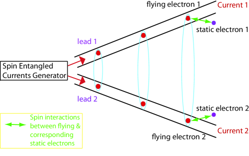
Figure 1: Illustration of our entanglement generation device. Two currents, composed of successive electron pairs that are maximally spin-entangled, emerge from a generator and pass down two leads. A static electron is situated downstream of the generator close to each lead, and the static pair is spatially well separated. The mobile spins in each lead interact with corresponding static spins as they pass. Note that the two flying spins of the same Bell pair are not required to, and will normally not, arrive at the sites of interaction with their corresponding static spins at the same time.

At the centre of our device is a spin-entangled current generator that outputs entangled pairs of spins $f_{i}$ down two different leads $i$. Each spin encounters a further, static, spin $s_{i}$ downstream of the generator and interacts with it, as shown in Fig. 1. The generator is based on earlier proposals of a passive device that produces pairs of spin-entangled electrons, with each pair maximally entangled in the singlet Bell state $|S\rangle_{f}=\frac{1}{\sqrt{2}}(|\uparrow_{f_{1}}\downarrow_{f_{2}}\rangle-|\downarrow_{f_{1}}\uparrow_{f_{2}}\rangle)$  [saraga03, oliver02, kolli09]. The nature of the static spins is not important, but one possibility is that a single electron is confined in each of the two quantum dots that are fixed close to the leads. Other suitable architectures include endohedral fullerenes in carbon nanotube peapods [watt08], carbon nanobud structures [nasibulin07], and surface acoustic waves whose minima isolate single electrons [barnes00].

2 Model and Basic Results

Let us start with an effective Hamiltonian coupling the flying and static spins of the following form:

$$H_{i}=\frac{g_{i}}{2}(\mathbf{\sigma}_{x}^{s_{i}}\mathbf{\sigma}_{x}^{f_{i}}+\mathbf{\sigma}_{y}^{s_{i}}\mathbf{\sigma}_{y}^{f_{i}})=g_{i}(\mathbf{\sigma}_{+}^{s_{i}}\mathbf{\sigma}_{-}^{f_{i}}+\mathbf{\sigma}_{-}^{s_{i}}\mathbf{\sigma}_{+}^{f_{i}})$$ (1)

where the $\sigma_{\pm}=(\mathbf{\sigma}_{x}\pm i\mathbf{\sigma}_{y})/2$ are the usual Pauli operators. The $g_{i}$ are $XY$ exchange coupling strengths that depend on the separation of the two spins. Each $g_{i}$ is time dependent since one of the two interacting spins is mobile. The time evolution operator $U_{i}(t)$ for a general state $|\Psi_{i}(t)\rangle=U_{i}(t)|\Psi_{i}(0)\rangle$ of the static-mobile pair $i$, is then

$$U_{i}(t)=\exp\left[-i\theta_{i}(t)(\mathbf{\sigma}_{+}^{s_{i}}\mathbf{\sigma}_{-}^{f_{i}}+\mathbf{\sigma}_{-}^{s_{i}}\mathbf{\sigma}_{+}^{f_{i}})\right],$$ (2)

where $\theta_{i}(t)=\int_{0}^{t}g_{i}(t^{\prime})dt^{\prime}/\hbar$. $\theta_{i}(t)$ is constant when $[0,t]$ is chosen so that $g_{i}(0)$ and $g_{i}(t)$ are negligible. In the basis $|\uparrow_{s_{i}}\uparrow_{f_{i}}\rangle$, $|\uparrow_{s_{i}}\downarrow_{f_{i}}\rangle$, $|\downarrow_{s_{i}}\uparrow_{f_{i}}\rangle$, $|\downarrow_{s_{i}}\downarrow_{f_{i}}\rangle$,

$$U_{i}=\left({\begin{array}[]{cccc}1&0&0&0\\ 0&\cos\theta_{i}&-i\sin\theta_{i}&0\\ 0&-i\sin\theta_{i}&\cos\theta_{i}&0\\ 0&0&0&1\\ \end{array}}\right).$$ (3)

2.1 Attractor

We first consider the case where $\theta_{1}=\theta_{2}=\theta$ and initially the static spins are in the state $|\uparrow_{s_{1}}\uparrow_{s_{2}}\rangle$. The starting state of the two static and the first pair of flying spins is then  $\frac{1}{\sqrt{2}}(|\uparrow_{s_{1}}\uparrow_{f_{1}}\rangle|\uparrow_{s_{2}}\downarrow_{f_{2}}\rangle-|\uparrow_{s_{1}}\downarrow_{f_{1}}\rangle|\uparrow_{s_{2}}\uparrow_{f_{2}}\rangle)$. Using the product of 2 unitary operators of the form of Eq. 3, we find that after interaction the state becomes $\cos\theta|\uparrow\uparrow\rangle_{s}|S\rangle_{f}-i\sin\theta|S\rangle_{s}|\uparrow\uparrow\rangle_{f}$. Since this first flying pair will no longer interact with the static spins nor with the following flying pairs, we can trace out this first flying pair to find the density matrix describing the static pair after the interaction: $\cos^{2}\theta|\uparrow\uparrow\rangle_{s}\langle\uparrow\uparrow|+\sin^{2}\theta|S\rangle_{s}\langle S|$.

In order to find the behaviour of our system for multiple passages of flying qubits, we require the following four maps which describe a single interaction event, $U_{1},U_{2}$:

$$|\uparrow\uparrow\rangle_{s}\langle\uparrow\uparrow| \mapsto \cos^{2}\theta\ |\uparrow\uparrow\rangle_{s}\langle\uparrow\uparrow|+\sin^{2}\theta\ |S\rangle_{s}\langle S|;$$

$$|\downarrow\downarrow\rangle_{s}\langle\downarrow\downarrow| \mapsto \cos^{2}\theta\ |\downarrow\downarrow\rangle_{s}\langle\downarrow\downarrow|+\sin^{2}\theta\ |S\rangle_{s}\langle S|;$$

$$|S\rangle_{s}\langle S| \mapsto \frac{1}{4}\sin^{2}2\theta\bigg{(}|\uparrow\uparrow\rangle_{s}\langle\uparrow\uparrow|+|\downarrow\downarrow\rangle_{s}\langle\downarrow\downarrow|\bigg{)}+\sin^{4}\theta\ |T_{0}\rangle_{s}\langle T_{0}|+\cos^{4}\theta\ |S\rangle_{s}\langle S|;$$

$$|T_{0}\rangle_{s}\langle T_{0}| \mapsto |T_{0}\rangle_{s}\langle T_{0}|,$$ (4)

where $|T_{0}\rangle=\frac{1}{\sqrt{2}}(|\uparrow\downarrow\rangle+|\downarrow\uparrow\rangle)$, another maximally entangled Bell state. These maps imply that the state $|T_{0}\rangle_{s}$ is an attractor for this process, and by tracking the states of the static spins through multiple passages of the flying spins it is clear that the system will converge towards this maximally entangled attractor; we need not consider any further maps since other static spin states are never accessed. This fixed point is also consistent with spin-invariant scattering of the flying singlets from a static $|T_{0}\rangle$ triplet, as can be verified directly from the Schrödinger equation.

2.2 Convergence

We now calculate the probabilities of obtaining the $|T_{0}\rangle_{s}$ state after a number of flying spin passages. The reduced density operator for the static spins after n iterations is, by definition, $\rho_{s}^{(n)}={\bf P}_{n}\centerdot\mathscr{P}$, where $\mathscr{P}\equiv\bigg{(}|\uparrow\uparrow\rangle_{s}\langle\uparrow\uparrow|,|\downarrow\downarrow\rangle_{s}\langle\downarrow\downarrow|,|S\rangle_{s}\langle S|,|T_{0}\rangle_{s}\langle T_{0}|\bigg{)}^{T}$ is the vector of projection operators for the base states and ${\bf P}_{n}\equiv\big{(}P_{\uparrow\uparrow}(n),\,P_{\downarrow\downarrow}(n),\,P_{S}(n),\,P_{T_{0}}(n)\big{)}^{T}$ is the corresponding vector of probabilities. Under the map, Eq. 4, $\mathscr{P}\mapsto L\mathscr{P}$ and hence $\rho_{s}^{(n)}\mapsto\rho_{s}^{(n+1)}={\bf P}_{n}\centerdot(L\mathscr{P})=(L^{T}{\bf P}_{n})\centerdot\mathscr{P}$, i.e.,

$${\bf P}_{n}\mapsto{\bf P}_{n+1}={\bf M_{0}}{\bf P}_{n}$$ (5)

where, by direct substitution,

$${\bf M_{0}}\equiv L^{T}=\left({\begin{array}[]{cccc}\cos^{2}\theta&0&\frac{1}{4}\sin^{2}2\theta&0\\ 0&\cos^{2}\theta&\frac{1}{4}\sin^{2}2\theta&0\\ \sin^{2}\theta&\sin^{2}\theta&\cos^{4}\theta&0\\ 0&0&\sin^{4}\theta&1\\ \end{array}}\right).$$

Note that the map, Eq. 5, preserves total probability, as it should. Since the matrix ${\bf M_{0}}$ describes the evolution of the state probabilities, its eigenvalues $\lambda_{i}$ must satisfy $|\lambda_{i}|\leqslant 1$. Except when $\theta$ is a multiple of $\pi$, there is always one (and only one) eigenvalue equal to unity, and the corresponding eigenvector is then our attractor state $|T_{0}\rangle\langle T_{0}|$. Using Mathematica and Eq. 5, we have derived closed analytic expressions for ${\bf M_{0}}^{n}$ and $P_{T_{0}}(n)$. For the initial conditions ${\bf P}_{0}=(1,0,0,0)^{T}$, we have

$$1-P_{T_{0}}(n)=2^{-4n-1}[(B^{n}+C^{n})-\frac{5+\cos 2\theta}{A}(B^{n}-C^{n})]$$ (6)

where

$$A=\sqrt{2\cos^{2}\theta(17+\cos 2\theta)}$$

$$B=7+8\cos 2\theta+\cos 4\theta-4A\sin^{2}\theta$$

$$C=7+8\cos 2\theta+\cos 4\theta+4A\sin^{2}\theta.$$ (7)

For large $n$, when $(4A\sin^{2}\theta)/(7+8\cos 2\theta+\cos 4\theta)\in(0,2)$, i.e., when $\theta\lesssim 0.89$, $C^{n}$ dominates over $B^{n}$ and we have

$$\ln\bigg{(}1-P_{T_{0}}(n)\bigg{)}\simeq\alpha(\theta)\ n+\beta(\theta)$$ (8)

where $\alpha(\theta)=\ln(C/16)\leqslant 0$ and $\beta(\theta)=\ln[(A+5+\cos 2\theta)/(2A)]$. For $\theta\ll 1$, $(5+\cos 2\theta)/A\to 1$, and $\beta(\theta)\to 0$. We plot the probability of obtaining the $|T_{0}\rangle_{s}\langle T_{0}|$ state against $\theta$, for different values of $n$ in Fig. 2.

$\begin{array}[]{cc}\begin{@subfigure}\includegraphics[width=180.67499pt]{Figure2.eps}\end{@subfigure}&\begin{@subfigure}\includegraphics[width=180.67499pt]{Figure3.eps}\@@toccaption{{\lx@tag[ ]{{(a)}}{$ $$\theta= 0.1$}}}\@@caption{{\lx@tag[ ]{{\footnotesize(a)}}{\footnotesize$ $$\theta= 0.1$}}}\end{@subfigure}\end{array}$

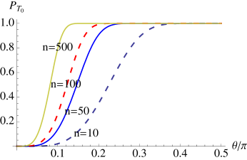
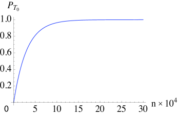
(a) θ= 0.1

$\begin{array}[]{cc}\begin{@subfigure}\includegraphics[width=180.67499pt]{Figure4.eps}\@@toccaption{{\lx@tag[ ]{{(b)}}{$ $$\theta= 0.03$}}}\@@caption{{\lx@tag[ ]{{\footnotesize(b)}}{\footnotesize$ $$\theta= 0.03$}}}\end{@subfigure}&\begin{@subfigure}\includegraphics[width=180.67499pt]{Figure5.eps}\@@toccaption{{\lx@tag[ ]{{(c)}}{$ $$\theta= 0.01$}}}\@@caption{{\lx@tag[ ]{{\footnotesize(c)}}{\footnotesize$ $$\theta= 0.01$}}}\end{@subfigure}\end{array}$

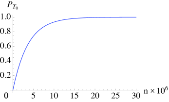
(b) θ= 0.03

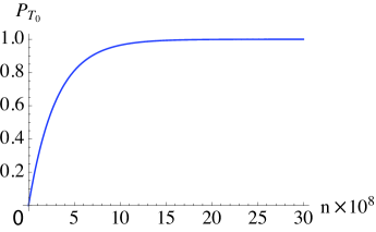
(c) θ= 0.01

Figure 2: Plots of the probabilites of obtaining the $|T_{0}\rangle_{s}\langle T_{0}|$ state (a) against $\frac{\theta}{\pi}$, after $10,50,100,500$ rounds of interactions, respectively; (b) - (d) against the number of rounds of interactions, $n$, for $\theta=0.1$, $0.03$ and $0.01$, respectively.

As the number of rounds increases, the range of $\theta$ values for which there is a high probability of obtaining the static $|T_{0}\rangle$ state becomes wider; we plot the probability $P_{T_{0}}(n)$ against the number of rounds, $n$, for some weak coupling strengths in Fig. 2(b)-(d). For the tunnelling rates $\Gamma$ in [herrmann10], the time interval $t_{0}$ between successive flying qubits are on the order of $\frac{\hbar}{\Gamma}\simeq 67$ ps, and therefore the time it takes for the static spins to converge to the $|T_{0}\rangle$ state would be 20 $\mu$s, 2 ms and 0.2 s for $\theta=0.1$, 0.03 and 0.01, respectively. These time intervals $t_{0}$ are at least one order less in [hofstetter09], and have the potential of being shortened further. Within the electron spin coherence time ($\geq 200$ $\mu$s) observed in [bluhm10], the convergence can occur for $\theta$ as small as 0.03 with the tunnelling rates achieved in [hofstetter09]. We also point out that molecular systems have the potential for phase shifts $\theta\gtrsim 1$ due to larger exchange interactions arising from nanometer length scales; for example the exchange coupling in a nanotube/fullerene system may be several orders of magnitudes greater than in gated semiconductor devices [ge08].

3 Generalisations

Let us now generalize our analysis, to include arbitrary coupling strengths ($\theta_{1}\neq\theta_{2}$), and arbitrary starting states for the static qubits. With the time evolution operators $U_{i}$ defined as in Eq. 3, we can find a completely positive map $\mathcal{L}_{s}$ which represents the effect on the static spin density operator $\rho_{s}$ of a passing flying qubit pair:

$$\rho_{s}^{(k+1)}=\mathcal{L}_{s}[\rho_{s}^{(k)}]=\Tr_{f}[(U_{1}\bigotimes U_{2})(\rho_{s}^{(k)}\bigotimes\rho_{f}^{(k)})(U_{1}\bigotimes U_{2})^{\dagger}]$$ (9)

where $\Tr_{f}$ denotes the partial trace [nielsen00] over the mobile spins, and $\rho_{f}=|S\rangle_{f}\langle S|$.

Eq. 9 corresponds to a set of 16 recurrence relations for the elements of $\rho_{s}^{(k)}$. When $\theta_{1}=\theta_{2}$, four of these relations decouple from all the others, as we found in our argument earlier. The superoperator $\mathcal{L}_{s}$ is not a linear map, and we thus vectorize the density operator states by listing the entries in the following order as a column vector: $(\rho_{11}\rho_{12}...\rho_{14}\rho_{21}...\rho_{24}\rho_{31}......\rho_{44})^{T}=:\tilde{\rho}$. The map corresponding to the action of the superoperator $\mathcal{L}_{s}$,

$$\tilde{\mathcal{L}}_{s}:\tilde{\rho}_{s}^{(k)}\longmapsto\tilde{\rho}_{s}^{(k+1)}$$ (10)

is then linear and can be written as a simple $16\times 16$ matrix M, whose entries can be easily calculated using Eq. 9.

We find that M always has an eigenvalue $\lambda=1$, independent of the values of the coupling strengths. The multiplicity of this eigenstate is one, unless $\theta_{1}$ and $\theta_{2}$ are multiples of $\pi$. The corresponding eigenvector $\tilde{\rho_{1}}$ is then a single attractor state that is independent of the initial configuration of the static spins, which when transformed back to its density matrix form is

$$\rho_{1}=\frac{1}{2(a+b)}\left({\begin{array}[]{cccc}a&0&0&0\\ 0&b&\frac{1}{\sqrt{2}}&0\\ 0&\frac{1}{\sqrt{2}}&b&0\\ 0&0&0&a\\ \end{array}}\right)$$ (11)

where

$$a=\frac{(\cos\theta_{1}-\cos\theta_{2})^{2}(1+\cos\theta_{1}\cos\theta_{2})\csc^{3}\theta_{1}\csc^{3}\theta_{2}}{2\sqrt{2}}\geq 0,$$

$$b=\frac{\csc\theta_{1}\csc\theta_{2}(\csc^{2}\theta_{1}+\csc^{2}\theta_{2})-\cot\theta_{1}\cot\theta_{2}(2+\csc^{2}\theta_{1}+\csc^{2}\theta_{2})}{2\sqrt{2}}\geq\frac{1}{\sqrt{2}}.$$ (12)

When $\theta_{1}=\theta_{2}$, we have $a=0$ and $b=\frac{1}{\sqrt{2}}$, and $\rho_{1}$ reduces the $|T_{0}\rangle\langle T_{0}|$ state as in the simple case. When $\theta_{1},\theta_{2}\in(0,\pi/2]$, all the other eigenvalues are numerically in the range $(-1,1)$, and their corresponding eigenvectors, when back in matrix form, all have trace zero and hence do not correspond to physical density operators. This has to be the case, as can be seen from the following argument. We can express any density state as $\rho=\sum_{i=1}^{16}a_{i}\rho_{i}$, since the set of eigenvectors $\tilde{\rho_{i}}$ (vectorized $\rho_{i}$) form a basis for M. The coefficients $a_{i}$ can take any values, so long as $\Tr(\rho)=1$ and $\rho$ is positive semi-definite and Hermitian. Hence, $\mathcal{L}_{s}[\rho]=\sum_{i=1}^{16}a_{i}\lambda_{i}\rho_{i}$, or more generally $\mathcal{L}_{s}^{n}[\rho]=\sum_{i=1}^{16}a_{i}\lambda_{i}^{n}\rho_{i}$, which also has trace 1 as a density matrix. As $n\rightarrow\infty$, $\lambda_{i}^{n}\rightarrow 0$ $\forall|\lambda_{i}|<1$ which is when $i=2,3,...,16$, and thus $\mathcal{L}_{s}^{n}[\rho]\rightarrow a_{1}\rho_{1}$. So, $\Tr(\mathcal{L}_{s}^{n}[\rho])\rightarrow a_{1}$ since we defined $\Tr(\rho_{1})=1$, and this requires $a_{1}=1$. We thus obtain $\rho=\rho_{1}+\Sigma_{i=2}^{16}a_{i}\rho_{i}$, and the trace requirement result in $\Sigma_{i=2}^{16}a_{i}\Tr(\rho_{i})=0$, which holds for various combinations of $a_{i}$’s. This can only be true when $\Tr(\rho_{i})=0$ $\forall i=2,3,...,16$. $\square$.

$\begin{array}[]{cc}\begin{@subfigure}\includegraphics[width=158.99377pt]{Figure6.eps}\@@toccaption{{\lx@tag[ ]{{(a)}}{Fidelity}}}\@@caption{{\lx@tag[ ]{{\footnotesize(a)}}{\footnotesize Fidelity}}}\end{@subfigure}&\begin{@subfigure}\includegraphics[width=158.99377pt]{Figure7.eps}\@@toccaption{{\lx@tag[ ]{{(b)}}{$E_{F}$}}}\@@caption{{\lx@tag[ ]{{\footnotesize(b)}}{\footnotesize$E_{F}$}}}\end{@subfigure}\end{array}$

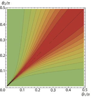
(a) Fidelity

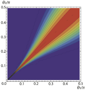
(b) E_F

Figure 3: Contour plots of (a) the fidelity between the attractor $\rho_{1}$ and the $|T_{0}\rangle\langle T_{0}|$ state; and (b) the entanglement of formation $E_{F}$ of $\rho_{1}$; each are plotted as a function of $\theta_{1}$ and $\theta_{2}$ $\in(0,\pi/2]$.

Now, we can find how close $\rho_{1}$ is to the $|T_{0}\rangle\langle T_{0}|$ state, for various values of $\theta_{1}$ and $\theta_{2}$, by calculating the fidelity $F$ as defined in [jozsa94]. In our case, we have

$$F(\rho_{1},|T_{0}\rangle\langle T_{0}|)=\Tr\bigg{(}\sqrt{\sqrt{\rho_{1}}|T_{0}\rangle\langle T_{0}|\sqrt{\rho_{1}}}\ \bigg{)}=\sqrt{\frac{b+\frac{1}{\sqrt{2}}}{2(a+b)}}$$ (13)

which takes a value of unity when $\theta_{1}=\theta_{2}$, as expected. Its contour plot in Fig. 3(a) illustrates that even when $\theta_{1}$ and $\theta_{2}$ are different, $\rho_{1}$ is still very close to the $|T_{0}\rangle\langle T_{0}|$ state for any $(\theta_{1},\theta_{2})$ in the central region. The fidelity values also indicate the levels of degradation in our entangled resource through unequal coupling, the degree of which can be further established by calculating the Entanglement of Formation [wootters98] $E_{F}$ that the bipartite state $\rho_{1}$ has [munro01]. We construct the contour plot for $E_{F}$ in Fig. 3(b) showing that the degree of entanglement $\rho_{1}$ possesses is very large, higher than 0.9, for any $(\theta_{1},\theta_{2})$ in the central red region.

$\begin{array}{ccc}& & \end{array}$

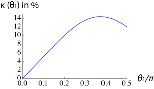
(a) Condition

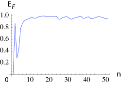
(b) randomθ_i ∈(1.2, 1.4)

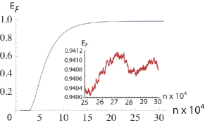
(c) rando