A submillimetre survey of the kinematics of the Perseus molecular cloud – III. Clump kinematics

Abstract

We explore the kinematic properties of dense continuum clumps in the Perseus molecular cloud, derived from our wide-field C¹⁸O $J=3\to 2$ data across four regions – NGC 1333, IC348/HH211, L1448 and L1455. Two distinct populations are examined, identified using the automated algorithms clfind (85 clumps) and gaussclumps (122 clumps) on existing SCUBA 850 µm data. These kinematic signatures are compared to the clumps’ dust continuum properties. We calculate each clump’s non-thermal linewidth and virial mass from the associated C¹⁸O $J=3\to 2$ spectrum. The clumps have supersonic linewidths, $\langle\sigma_{\mathrm{NT}}/c_{\mathrm{s}}\rangle=1.76\pm 0.09$ (clfind population) and $1.71\pm 0.05$ (with gaussclumps). The linewidth distributions suggest the C¹⁸O line probes a lower-density ‘envelope’ rather than a dense inner core. Similar linewidth distributions for protostellar and starless clumps implies protostars do not have a significant impact on their immediate environment. The proximity to an active young stellar cluster seems to affect the linewidths: those in NGC 1333 are greater than elsewhere. In IC348 the proximity to the old IR cluster has little influence, with the linewidths being the smallest of all. The virial analysis suggests that the clumps are bound and close to equipartition, with virial masses similar to the masses derived from the continuum emission. In particular, the starless clumps occupy the same parameter space as the protostars, suggesting they are true stellar precursors and will go on to form stars. We also search for ordered C¹⁸O velocity gradients across the face of each core. Approximately one third have significant detections, which we mainly interpret in terms of rotation. However, we note a correlation between the directions of the identified gradients and outflows across the protostars, indicating we may not have a purely rotational signature. The fitted gradients are in the range ${\cal G}=1$ to 16 km s^-1 pc^-1, larger than found in previous work, probably as a result of the higher resolution of our data and/or outflow contamination. These gradients, if interpreted solely in terms of rotation, suggest that the rotation is not dynamically significant: the ratios of clump rotational to gravitational energy are $\beta_{\mathrm{rot}}\lesssim 0.02$. Furthermore, derived specific angular momenta are smaller than observed in previous studies, centred around $j\sim 10^{-3}$ km s^-1 pc, which indicates we have identified lower levels of rotation, or that the C¹⁸O $J=3\to 2$ line probes conditions significantly denser and/or colder than $n\sim 10^{5}$ cm^-3 and $T\sim 10$ K.

1 Introduction

Stars form inside dense cores deep within molecular clouds. The similarity of the core mass function (CMF) to the initial mass function of stars (IMF, see Motte, Andre & Neri 1998; Alves, Lombardi & Lada 2007) has sometimes been used (e.g. Enoch et al. 2008) as evidence against theories of core formation where no correspondence is anticipated, e.g. in the competitive accretion picture (Bonnell et al., 2001; Bate & Bonnell, 2005). However, the mapping of a given CMF on to the resultant IMF is complicated by many factors (see e.g. Hatchell & Fuller 2008; Curtis & Richer 2010), such as the cores’ varying multiplicity (Goodwin et al., 2008), star-forming efficiencies (Swift & Williams, 2008) and/or mass-dependent lifetimes (Clark, Klessen & Bonnell, 2007). In fact, as shown by Swift & Williams (2008) and Goodwin & Kouwenhoven (2009), diverse evolutionary schemes can map the observed CMFs on to the IMF, implying the current mass function data are not sufficient to discriminate between different theoretical models by themselves.

The kinematics of star-forming cores, probed with spectral-line observations of dense molecular tracers, are arguably the best discriminator between different models of core formation (e.g. André et al. 2007; Kirk, Johnstone & Tafalla 2007). For example, cores created by shocks in large-scale flows exhibit large velocity gradients and are located at local maxima in the line-of-sight velocity dispersion (e.g. Ballesteros-Paredes, Klessen & Vázquez-Semadeni 2003; Klessen et al. 2005). Alternatively, the magnetically controlled scenario has more quiescent velocity fields (e.g. Nakamura & Li, 2005), well-matched to observations of isolated starless cores with subsonic levels of turbulence (e.g. Myers, 1983; Caselli et al., 2002). Such quiescent cores are in opposition to purely hydrodynamic models of gravoturbulent fragmentation (see Mac Low & Klessen, 2004) which produce a majority of cores with supersonic velocity dispersions.

Offner, Klein & McKee (2008a) and Krumholz, McKee & Klein (2005) maintain that the physical mechanism of star formation depends on the much debated presence (or absence) of turbulent feedback. In one view, molecular clouds are short-lived (on timescales of order one dynamical time), non-equilibrium structures (e.g. Elmegreen et al., 2000; Hartmann, 2001; Dib et al., 2007) characterized by transient turbulence, which dissipates quickly. In this scenario, stars could form by the collapse of discrete cores. Conversely, molecular clouds might form slowly and be quasi-equilibrium objects (see e.g. Shu, Adams & Lizano, 1987; McKee, 1999; Krumholz & Tan, 2007; Nakamura & Li, 2007). This would require turbulence to be constantly injected into the clouds, either externally (from e.g. supernova blast waves or Hii regions) or internally (from e.g. protostellar outflows) and cores could form through competitive accretion (Bonnell et al., 2001). Offner et al. (2008b) demonstrate that these two disparate views of star formation give rise to distinguishable kinematics in dense stellar precursors and thus the study of core kinematics potentially offers a way to probe the turbulent state of the surrounding molecular cloud.

This paper is concerned with the kinematical properties of dense clumps in the Perseus molecular cloud (hereafter simply Perseus) and compares them to theoretical models. We examine the linewidths, virial masses and ordered velocity gradients of two populations of clumps (Curtis & Richer, 2010) identified across SCUBA dust continuum maps (Hatchell et al., 2005). These kinematic signatures are derived for each clump from our wide-field survey (Curtis, Richer & Buckle, 2010a, Paper I) of four clusters of star-forming cores towards NGC 1333, IC348/HH211 (simply IC348 hereafter), L1448 and L1455 in the $J=3\to 2$ rotational lines of CO and its common isotopologues ¹³CO and C¹⁸O. In the preceding paper of this series (Curtis et al. 2010b, Paper II), we explored the evolution of molecular outflows across these regions. We organize this paper as follows: the remainder of the introduction explains the naming conventions we have adopted to describe star-forming clumps/cores. §2 briefly describes the continuum data and associated clump catalogues alongside our spectral-line datasets, from which we derive the clump kinematics. Various clump kinematic signatures are investigated in §3, including the clumps’ linewidths (§3.1) and virial masses (§3.2), before we search for ordered velocity gradients across the face of the clumps in §3.3, which we interpret with a solid-body-rotation model. Finally, we summarize this work in §4.

1.1 Nomenclature and clump populations

We adhere to the clump hierarchy explained in Curtis & Richer (2010), which follows Williams, Blitz & McKee (2000). Briefly, molecular clouds contain clumps which in turn harbour cores, the direct precursors of individual or multiple stars. Clumps without embedded objects are starless, unless they are gravitationally bound when we refer to them as prestellar.

2 Observational data

2.1 Dust continuum

The SCUBA 850 µm data analysed have a beam size of 14 arcsec (0.017 pc at 250 pc, our adopted distance to Perseus, see Paper I) and are sampled on a 3 arcsec grid with a typical rms noise level, $\sigma_{\mathrm{rms}}=35$ mJy beam^-1 (Hatchell et al., 2005).

2.2 Clump catalogues

We investigate the kinematics of two populations of dust continuum clumps, which we identified in the SCUBA 850 µm data in a previous paper (Curtis & Richer, 2010), using the two most popular automated algorithms: clfind (Williams, de Geus & Blitz, 1994) and gaussclumps (Stutzki & Güsten, 1990). Our motivation in that study was to determine which clump properties can be robustly measured and which depend on the extraction technique. We continue that approach in this work, analysing the kinematic signatures for each population in turn.

In Curtis & Richer (2010), we located 85 and 122 clumps using clfind and gaussclumps respectively with peak flux densities $\geq 4\sigma_{\mathrm{rms}}=140$ mJy beam^-1, across the same areas where we also have C¹⁸O $J=3\to 2$ data (Paper I). The clumps were identified as starless, Class 0 or Class I protostars using the classifications of Hatchell et al. (2007, hereafter HFR07), which are based on source SEDs incorporating Spitzer data. We associate a clump with a HFR07 source, if the separation between the clump and HFR07 source peak positions is less than the clump’s diameter (see Curtis & Richer 2010). Given the similarities in the extraction method and resulting population, most of the clfind clumps are directly on top of the HFR07 sources and are unambiguously identified. However, three gaussclumps sources are large enough to encapsulate two HFR07 sources and their results are correspondingly included in the population statistics twice.

2.3 Spectral-line

The C¹⁸O $J=3\to 2$ observations used in this analysis were undertaken with HARP (the Heterodyne Array Receiver Project; Buckle et al., 2009) on the James Clerk Maxwell Telescope and have been described in detail previously (Paper I). Striping artefacts resulting from systematic differences in calibration between HARP channels were removed using a ‘flatfield’ procedure (fully described in Paper I). The final datasets are sampled on a 3 arcsec grid, distributed using a Gaussian gridding kernel with a 9 arcsec full-width half maximum (FWHM), yielding an equivalent beam size of 17.7 arcsec. The median rms spectral noise values, averaged across each region’s map (measured in 0.15 km s^-1 channels), are 0.18, 0.15, 0.15 and 0.14 K for NGC 1333, IC348, L1448 and L1455 respectively.

3 The kinematics of the SCUBA cores

In molecular clouds, the C¹⁸O $J=3\to 2$ line is expected to be optically thin and excited in dense regions ($n_{\mathrm{crit}}\sim 10^{4}$ cm^-3). It should therefore trace material in the vicinity of or within the dense agglomerations surveyed with SCUBA. At the peak of every clump in our two catalogues (see §2.2), we extracted the C¹⁸O $J=3\to 2$ spectrum and fitted a Gaussian profile to it using splat if the peak of the C¹⁸O line was $\geq 3\sigma_{\mathrm{sp}}$, where $\sigma_{\mathrm{sp}}$ is the rms spectral noise. We did not detect C¹⁸O at the $3\sigma$ level towards 4 (5 per cent) clfind and 6 (5 per cent) gaussclumps positions. Of the detections, 13 (15 per cent) clfind and 18 (15 per cent) gaussclumps spectra have double-peaked line profiles. For comparison, Kirk et al. (2007, hereafter KJT07) made pointed N₂H⁺ $J=1\to 0$ and C¹⁸O $J=2\to 1$ observations on the Institut de Radio Astronomie Millimétric (IRAM) 30-m telescope (with beam sizes of 25 and 11 arcsec respectively) towards 157 candidate cores in Perseus – 44 pointings in our fields – and found 66 (42 per cent) C¹⁸O spectra required two component Gaussian fits with three in one case. Generally, $J=2\to 1$ data trace lower density ($n_{\mathrm{crit}}\sim 10^{3}$ cm^-3) and/or colder material than the $3\to 2$ at lower optical depths by a factor of 2–3 in the optically thin limit. Therefore the $J=2\to 1$ line is unlikely to saturate if the $J=3\to 2$ data are optically thin. This suggests there are separate emitting sources along the line-of-sight with different temperatures and/or densities which require multiple-component fits for one transition and not the other. An alternative is simply that at our velocity resolution (0.15 km s^-1 compared to KJT07’s 0.05 km s^-1) many of KJT07’s separate components are blended into one, which might partly explain our larger linewidths (see §3.1).

3.1 Linewidths

The linewidths in molecular clouds are substantially larger than the sound speed of their constituent gas (e.g. Zuckerman & Evans, 1974; Solomon et al., 1987). Such supersonic linewidths are thought to arise from chaotic and/or turbulent motions of unknown fundamental origin (see Elmegreen & Scalo, 2004 and references therein). The velocity dispersion in a region scales with its size (e.g. Larson, 1981) akin to the Kolmogorov law for subsonic incompressible turbulence, although turbulence in the interstellar medium is actually highly compressible and often supersonic causing shocks. However, dense star-forming cores harboured in cloud interiors possess near-thermal linewidths almost devoid of the turbulent movements that cause the broadening in their outer envelopes (e.g. Benson & Myers, 1989; Barranco & Goodman, 1998; Goodman et al., 1998; Pineda et al., 2010). The C¹⁸O $J=3\to 2$ transition is expected to probe a region intermediate in scale between the dense core and its environment, although it is not the tracer of choice for young prestellar cores. In the cold ($\la 10$ K), high-density ($\geq 10^{5}$ cm^-3) centres of such objects, the conditions may result in depletion, where many molecules (including CO and its isotopologues) freeze-out on to dust grains. Such zones are better probed by molecules such as N₂H⁺and H₂D⁺, but in any case the CO $J=3\to 2$ transitions should probe higher densities than lower $J$ ones.

We take a core’s total one-dimensional velocity dispersion, $\sigma_{\mathrm{C^{18}O}}$ to be the quadrature sum of its thermal and non-thermal dispersions, $\sigma_{\mathrm{T}}$ and $\sigma_{\mathrm{NT}}$ respectively:

$$\sigma_{\mathrm{C^{18}O}}^{2}=\sigma_{\mathrm{T}}^{2}+\sigma_{\mathrm{NT}}^{2}.$$ (1)

To find $\sigma_{\mathrm{NT}}$ (plotted in Fig. 1), we calculate $\sigma_{\mathrm{T}}$:

$$\sigma_{\mathrm{T}}^{2}=\frac{kT}{m_{\mathrm{C^{18}O}}m_{\mathrm{p}}},$$ (2)

where $m_{\mathrm{p}}$ is the mass of a proton and $m_{\mathrm{C^{18}O}}$ the relative molecular mass of C¹⁸O ($m_{\mathrm{C^{18}O}}=30$). The clump temperature, $T$, is taken from the kinetic temperatures of ammonia gas (Rosolowsky et al., 2008), where available, or 10 K and 15 K for identified starless and protostellar cores respectively where not. For those clumps without a HFR07 association we assume a temperature of 12 K. We calculate the turbulent fraction, plotted in Figs. 2 to 5, $f_{\mathrm{turb}}=\sigma_{\mathrm{NT}}/c_{\mathrm{s}}$, where $c_{\mathrm{s}}=\sqrt{\gamma kT/\bar{m}m_{\mathrm{p}}}$ is the thermal sound speed in the bulk of the gas of mean molecular mass $\bar{m}=2.33m_{\mathrm{p}}$ (assuming 1 He for every 5 H₂) and $\gamma$ the adiabatic index ($\sim 7/5$ for a diatomic molecule). For $T=10$ K, $c_{\mathrm{s}}=0.22$ km s^-1 and at 15 K $c_{\mathrm{s}}=0.27$ km s^-1. Summaries of $f_{\mathrm{turb}}$ for various populations are listed in Tabs. 1 and 2.

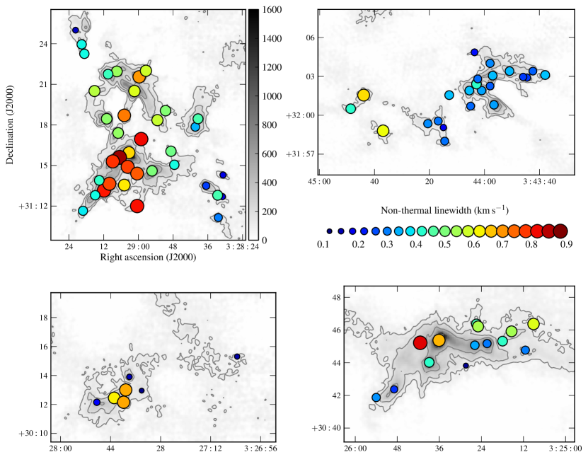
Figure 1: Spatial distribution of C¹⁸O non-thermal linewidth across NGC 1333 (upper left), IC348 (upper right), L1448 (lower right) and L1455 (lower left). The grey-scale is SCUBA 850 µm flux density in mJy beam^-1 (Hatchell et al., 2005) with contours at 100, 200, 400, 800, 1600 and 3200 mJy beam^-1. Circles are positioned at the peak of every SCUBA clump in our catalogue identified using clfind (Curtis & Richer, 2010) where there is a $3\sigma$ C¹⁸O detection. The circles’ size and colour reflect the linewidth as shown in the key.

A majority of the linewidths are supersonic with means $\langle f_{\mathrm{turb}}\rangle=1.76\pm 0.09$ and $1.71\pm 0.05$ for the clfind and gaussclumps populations respectively. The level of non-thermal broadening should take into account motions from both: (a) the source itself i.e. infall, rotation and outflows and (b) the source’s natal environment. Young stars can inject significant energy into their surroundings, increasing the non-thermal motions within nearby star-forming cores. For example Caselli & Myers (1995) found an inverse relationship between a core’s NH₃ linewidth and the distance to the nearest young stellar cluster in Orion B. There are three such young clusters in Perseus (see Hatchell et al., 2005): IC348, NGC 1333 and the Per OB2 association. Therefore, of our fields, NGC 1333 and IC348 are very near to young clusters, while L1448 and L1455 are further away (L1455 being the furthest).

Table 1: Summary of the turbulent fractions, $f_{\mathrm{turb}}$, derived from Gaussian fits to the C¹⁸O $J=3\to 2$ line at the peak of every SCUBA clump identified with clfind (Curtis & Richer, 2010). The results are broken into either different regions in Perseus or clump classifications (see §2.2). The quoted errors ($\sigma$) are errors on the mean ($\sigma/\sqrt{N}$) not sample deviations.

Population	Number	$f_{\mathrm{turb}}$	$\sigma_{f}$
All	81	1.76	0.09
NGC 1333	37	2.05	0.12
IC348	23	1.36	0.09
L1448	14	1.8	0.2
L1455	7	1.5	0.4
Starless	17	1.8	0.2
Protostars†	33	1.89	0.12
Class 0	19	2.04	0.16
Class I	14	1.7	0.2

^† The Class 0 and I populations combined.

Table 2: Summary of the turbulent fractions, $f_{\mathrm{turb}}$, for the gaussclumps clump population as in Tab. 1.

Population	Number	$f_{\mathrm{turb}}$	$\sigma_{f}$
All	119	1.71	0.05
NGC 1333	64	1.91	0.07
IC348	25	1.44	0.07
L1448	23	1.52	0.13
L1455	7	1.5	0.3
Starless	24	1.61	0.11
Protostars	40	1.80	0.10
Class 0	27	1.73	0.11
Class I	13	2.0	0.2

The variations in $f_{\mathrm{turb}}$ region-to-region (see Fig. 2), which we might attribute to each region’s distance from a young stellar cluster, are slightly different for the two populations. For the clfind clumps (see Tab. 1), NGC 1333 and L1448 have statistically similar fractions: $2.05\pm 0.12$ and $1.8\pm 0.2$ respectively. We ignore the L1455 populations in these comparisons as they are so few in number. IC348, on the other hand, has much smaller linewidths overall: $\langle f_{\mathrm{turb}}\rangle=1.36\pm 0.09$. The gaussclumps population (see Tab. 2) has clumps in NGC 1333 with much larger turbulent fractions than the similar $f_{\mathrm{turb}}$ means in IC348 and L1448: $1.91\pm 0.07$ compared to $1.44\pm 0.07$ and $1.52\pm 0.13$. Therefore, for both populations, the IC348 linewidths are smaller than in NGC 1333, even though both regions are close to stellar clusters. This is possibly (as noted in Paper I) because the IC348 IR cluster is old and no longer actively forming stars, so it affects its environs much less than the NGC 1333 cluster. There is a wide range of clump $f_{\mathrm{turb}}$ in L1448, which could be a result of a significant contribution to the C¹⁸O linewidth from molecular outflows. Many of the protostellar clumps in L1448 drive particularly strong flows (Paper II).

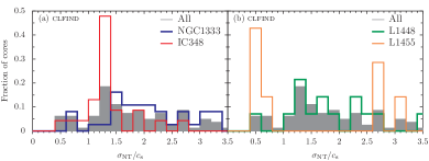
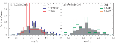
Figure 2: Distribution of clump turbulent fractions, $f_{\mathrm{turb}}=\sigma_{\mathrm{NT}}/c_{\mathrm{s}}$, measured from the HARP C¹⁸O $J=3\to 2$ data (see text), broken down by region for the clfind (upper panels) and gaussclumps populations (lower panels).

On dividing the clumps into protostellar and starless subsets (see Fig. 3), there appears to little difference between the distributions of turbulent fraction for both source types and clump populations. At the peak positions of the clfind objects, we find $\langle f_{\mathrm{turb}}\rangle=1.8\pm 0.2$ for starless clumps compared to $1.89\pm 0.12$ for protostars. Similarly, $\langle f_{\mathrm{turb}}\rangle=1.61\pm 0.11$ and $1.80\pm 0.10$ for starless and protostellar gaussclumps sources respectively. Further separation of the protostars into Class 0 and I clumps does not yield statistical differences between their average $f_{\mathrm{turb}}$ (see Tabs. 1 and 2). Unfortunately, such simple averages do not provide the whole picture we can see in the distributions (in Fig. 3). For example, if the small but significant population of high $f_{\mathrm{turb}}$ starless cores were eliminated it would seem that protostars have marginally higher $f_{\mathrm{turb}}$ on average. However, the large uncertainties on the average $f_{\mathrm{turb}}$ do emphasize the need for larger samples of objects. For the clfind population (but not the gaussclumps sources) most of the high $f_{\mathrm{turb}}$ protostars are Class 0, and all of the low $f_{\mathrm{turb}}$ Class I, which is perhaps what we might expect if outflow power decreases from the Class 0 to I stage (Bontemps et al. 1996; Paper II). Overall, there are few significant differences between the starless and protostellar distributions.

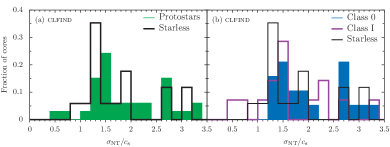
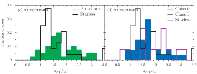
Figure 3: Distribution of clump turbulent fractions, $f_{\mathrm{turb}}=\sigma_{\mathrm{NT}}/c_{\mathrm{s}}$, measured from the HARP C¹⁸O $J=3\to 2$ data (see text), broken down by the different source types for the clfind (upper panels) and gaussclumps populations (lower panels).

We can draw interesting comparisons with the C¹⁸O ($J=2\to 1$) and N₂H⁺ $f_{\mathrm{turb}}$ distributions presented by KJT07 (see Figs. 4 and 5). Our distributions are closer to the C¹⁸O distributions of KJT07 than their N₂H⁺ results. The high levels of non-thermal motions, shown by some of our sources, are simply not present in N₂H⁺ data. A striking contrast between the C¹⁸O distributions is that many of our cores have high $f_{\mathrm{turb}}$ ($\geq 3.5$), which are not seen for either protostars or starless cores by KJT07. In addition, many KJT07 starless cores have sub-thermal linewidths ($f_{\mathrm{turb}}$$<1$). These differences may be partly caused by the spectral resolution of our observations ($\Delta v=0.15$ km s^-1 compared to KJT07’s 0.05 km s^-1), rather than intrinsically different results. Our slightly poorer resolution means we cannot probe as narrow linewidths and we possibly blend many of the separate components, noted in KJT07’s C¹⁸O spectra, into one. Given the similarities it seems likely our C¹⁸O $J=3\to 2$ data probe the same regions as the $J=2\to 1$ observations of KJT07, namely the outer parts of star-forming cores, referred to by KJT07 as their envelopes. This is probably because of C¹⁸O freeze-out in the dense, cold interiors of star-forming cores. Such regions should see an enhancement in the abundance of say N₂H⁺ relative to C¹⁸O. KJT07 investigated this possibility for their similar population of candidate cores in Perseus by measuring the variation in the integrated C¹⁸O-to-N₂H⁺ ratio with peak SCUBA flux density (an approximate proxy for central H₂ volume density). They found high C¹⁸O-to-N₂H⁺ ratios (i.e. little C¹⁸O depletion) occurred mainly in starless cores, which have the smallest SCUBA fluxes (i.e. lowest densities), whereas high-flux cores (mainly protostars) have low ratios suggesting high levels of C¹⁸O depletion.

Given that our starless and protostellar C¹⁸O distributions are quite similar, we may also conclude (like KJT07) that protostars do not affect their environment significantly. The starless distribution may differ from the true prestellar one as starless clumps with the largest linewidths are likely to be unbound, and thus the true prestellar turbulent fractions will be smaller. Finally, we also note little correspondence with the simulations of Klessen et al. (2005), whose results for a large-scale driven (LSD) gravoturbulent model are also plotted in Figs. 4 and 5. KJT07 claim to have a good fit to the Klessen et al. data with their C¹⁸O starless population, although the model was designed to match N₂H⁺ observations.

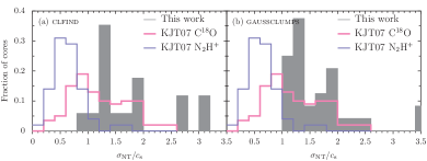
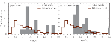
Figure 4: Distribution of $f_{\mathrm{turb}}$, for the starless clump populations identified with clfind (left panels) or gaussclumps (right panels), measured from the HARP C¹⁸O $J=3\to 2$ data. Overlaid for comparison are the distributions found by KJT07 for 157 candidate cores using C¹⁸O $J=2\to 1$ (upper panels, pink) and N₂H⁺ $J=1\to 0$ (upper panels, blue). A prediction for cores from the gravoturbulent simulation of Klessen et al. (2005) is also shown for turbulence driven on large scales (lower panels, brown). For that simulation the turbulent fraction extends beyond 3.5 to 4.3 (not plotted), though there are small numbers of clumps in those bins ($\sim 2$ per cent).

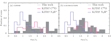
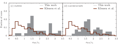
Figure 5: Distribution of $f_{\mathrm{turb}}$, for the protostellar clump populations identified with clfind (left panels) or gaussclumps (right panels), measured from the HARP C¹⁸O $J=3\to 2$ data. Overlaid for comparison are the distributions found by KJT07 for 157 candidate cores using C¹⁸O $J=2\to 1$ (upper panels, pink) and N₂H⁺ $J=1\to 0$ (upper panels, blue). A prediction for cores from the gravoturbulent simulation of Klessen et al. (2005) is also shown for turbulence driven on large scales (lower panels, brown). For that simulation the turbulent fraction extends beyond 3.5 to 4.3 (not plotted), though there are small numbers of clumps in those bins ($\sim 2$ per cent).

3.2 Virial theorem

If the C¹⁸O data trace material that will go on to form the final star and not just the ambient gas in which a YSO is embedded, the core linewidth can inform us about its stability, i.e. whether the cores are gravitationally bound. We can then distinguish bound, starless i.e. prestellar cores from unbound ones that will dissipate without forming a star.

The virial theorem is often used to examine this stability and we will apply it to our two populations of clumps identified in SCUBA 850 µm data. The clump virial mass, $M_{\mathrm{vir}}$, is used as an estimate of the internal energy of the clump whilst its dust mass at 850 µm, $M_{850}$, is as an estimate of the potential energy. If we assume that the linewidths only reflect gravity and we have spherical clumps the virial theorem is

$$M_{\mathrm{vir}}=\frac{a\sigma^{2}R}{G},$$ (3)

where $\sigma$ is the average three-dimensional velocity dispersion, $R$ the clump radius and $a$ a constant that depends on the form of the density profile (a derivation can be found in e.g. Binney & Tremaine, 2008; Rohlfs & Wilson, 2004). If we assume a power law density profile, $\rho(r)\propto r^{-n}$, then (e.g. MacLaren, Richardson & Wolfendale, 1988):

$$a=\frac{5-2n}{3-n}.$$ (4)

Provided the C¹⁸O line of FWHM, $\Delta v_{\mathrm{C^{18}O}}$, traces the bulk of the gas with a Gaussian velocity distribution and the same non-thermal linewidth as H₂, we can estimate

$$\sigma^{2}=\frac{3}{8\ln 2}\left(\Delta v_{\mathrm{C^{18}O}}^{2}+\frac{8\ln 2kT}{m_{\mathrm{p}}}\left(\frac{1}{\bar{m}}-\frac{1}{m_{\mathrm{C^{18}O}}}\right)\right),$$ (5)

where $m_{\mathrm{p}}$ is the proton mass, $\bar{m}=2.33$ to factor in the abundance of He relative to H₂ and $m_{\mathrm{C^{18}O}}=30$. This yields for a shallow power law clump, $n=1.5$, consistent with the shapes found by Enoch et al. (2008)

$$M_{\mathrm{vir}} = 3.4\left(\frac{a}{4/3}\right)\left(\left(\frac{\Delta v_{\mathrm{C^{18}O}}}{1\,\mathrm{km\,s^{-1}}}\right)^{2}+0.22\left(\frac{T}{12\,\mathrm{K}}\right)\right)$$ (6)

$$\qquad\times\left(\frac{R}{\mathrm{0.02\,pc}}\right)\,\mathrm{M_{\odot}.}$$

We expect objects in equipartition to have $M_{\mathrm{vir}}\sim M_{850}$ whilst those that are self-gravitating should have $M_{\mathrm{vir}}\la 2M_{850}$.

We take data on the clumps’ dust properties from Curtis & Richer (2010). Each clump’s 850 µm mass ($M_{850}$) assumes the dust is optically thin, has an opacity, $\kappa=0.012$ cm² g^-1 and is at a single temperature, $T_{\mathrm{D}}$. Again these temperatures are taken as the NH₃ kinetic temperatures (Rosolowsky et al., 2008), where available, or 10 K (for starless cores) and 15 K (for protostars) where not. The core radius, $R_{\mathrm{dec}}$, is the geometric mean of the two core semi-major and -minor axis ‘sizes’ each deconvolved with the beam size. These ‘sizes’ are the standard deviation of the pixel coordinates about the core centroid, weighted by the pixel values.

There are considerable uncertainties in any dust and virial mass estimates. The errors are very difficult to quantify for individual clumps without detailed modelling. Thus, we follow complementary studies (e.g. Buckle et al. 2010; Enoch et al. 2008) and do not attempt to account for the uncertainties in our analysis, except for a discussion of their magnitude, which follows. The dust masses depend on the assumed distance to Perseus and the dust properties (temperature and opacity). We try to minimize the effects of dust temperature by using the NH₃ kinetic temperature as an estimate of $T_{\mathrm{D}}$, which should be an accurate measurement at high volume densities ($\gtrsim 10^{4}$ cm^-3, e.g. Galli, Walmsley & Gonçalves 2002), where the gas and dust are thermally coupled. Nevertheless our dust temperature estimates still do not account for variations in the dust temperature across a clump. A range of distances have been used in the literature for Perseus (220 to 350 pc see e.g. Paper I) and indeed it may not be a contiguous cloud at a single distance. These result in an uncertainty of a factor of $\sim 5$ in the dust mass estimates. The virial masses depend on the assumed clump profile, with steeper profiles producing smaller masses, however it only varies by a factor of 1.7 between a constant density and $1/r^{2}$ profile. This combined with the uncertainties in the distance and linewidth produce again around a factor of $\sim 5$ in uncertainty. As we previously noted (§3.1), it is likely that the C¹⁸O $J=3\to 2$ line only traces the envelope of a clump, which could lead to an over-estimate of the non-thermal H₂ linewidth (compared to estimates from say NH₃ or N₂H⁺) and correspondingly the virial mass. Even if our estimates of the dust and virial masses were infallible, assuming that a clump with $M_{\mathrm{vir}}\gg M_{850}$ is unbound may be misleading; external pressure and/or magnetic fields may contain such a clump. For instance KJT07 calculate that cores with external pressures consistent with their previous Bonnor-Ebert sphere modelling (Kirk, Johnstone & Di Francesco, 2006), should be considered in equipartition not merely self-gravitating if $M_{\mathrm{vir}}\sim 2M_{850}$.

The C¹⁸O virial masses, which we plot in Fig. 6 against the 850 µm mass, lie in the range 0.8 to 22.9 M_⊙ for the clfind sources and 0.4 to 17.8 M_⊙ for the gaussclumps sources, reflecting their smaller radii. Most of the clumps lie scattered near the ‘equipartition’ line, $M_{\mathrm{vir}}=M_{850}$. The results are similar for the different algorithms, regions and evolutionary types (see Tables 3 and 4 for summaries of the population statistics). Least-squares straight-line fitting results in poorly-constrained power law exponents of 0.8–0.9 for almost all the correlations.

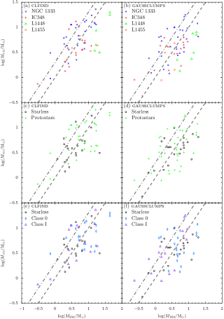
Figure 6: Virial mass versus clump dust mass for the clfind (left panels, (a), (c) and (e)) and gaussclumps (right panels, (b), (d) and (f)) populations, differentiated by region (top panels, (a) and (b)) or the classifications of HFR07 (the rest). Virial masses are estimated from the C¹⁸O $J=3\to 2$ linewidth at the catalogue positions of Curtis & Richer (2010). The masses are calculated using the temperatures from Rosolowsky et al. (2008) where possible or 10 and 15 K for starless and protostellar cores respectively where not. Lines denote where we expect cores to be in equipartition, i.e. $M_{\mathrm{vir}}=M_{850}$ (dashed) or the limit where they are self-gravitating, $M_{\mathrm{vir}}=2M_{850}$ (dot-dashed), although the reader should note the considerable uncertainties in both masses. Only clumps which have a HFR07 source association are plotted.

Given the uncertainties in both the virial and dust mass estimates, it is not possible to draw unequivocal conclusions about the stability of individiual clumps. However, we will compare distinct populations. The different regions show similar behaviour with a lot of scatter. The L1448 population is outlying for both algorithms with a high $M_{850}/M_{\mathrm{vir}}$ ratio. L1448 is interesting as it contains large SCUBA flux densities and massive outflows but has relatively weaker C¹⁸O emission. The NGC 1333 population has a smaller $M_{850}/M_{\mathrm{vir}}$ ratio than the others, which we might interpret as being more unbound and therefore transient, with a larger number of cores above the $M_{\mathrm{vir}}=M_{850}$ threshold. This could be a result of its more perturbed environment.

Protostellar clumps, by definition should be gravitationally bound. If starless clumps occupy a similar $M_{\mathrm{vir}}-M_{850}$ sample space, then this suggests that they too are a gravitationally bound population. In Fig. 6, the starless and protostellar clumps occupy the same regions of the plot and their mass ratios are very similar in Tabs. 3 and 4. This implies that the starless population is gravitationally bound as well and truly prestellar in nature (as found by Enoch et al. 2008).

The clumps also seem spread around the ‘equipartition’ line $M_{\mathrm{vir}}=M_{850}$. Approximate equipartition was also found by Caselli et al. (2002) in a sample of 60 starless cores using N₂H⁺ linewidths. Other studies e.g. the C¹⁸O cores looked at by Tachihara et al. (2002) found the virial mass considerably larger than the core mass estimate. The latter result is successfully explained by the gravoturbulent models of Klessen et al. (2005), who find a large majority of starless cores with $M_{\mathrm{vir}}\gg M$ for both large and small driving-scale turbulence models, with their protostellar sources non-coincident in parameter space at $M>M_{\mathrm{vir}}$. Our results would not favour such a model for Perseus, even in its clustered environment.

Table 3: Summary of virial mass statistics for the clfind SCUBA clumps identified in Curtis & Richer (2010), which have a HFR07 classification. All the quoted errors ($\sigma$) are errors on the mean ($\sigma/\sqrt{N}$) not simple sample deviations.

Population	No	$M_{\mathrm{vir}}$	$\sigma_{M}$	$M_{850}/M_{vir}$	$\sigma_{\mathrm{ratio}}$
		(M⊙)	(M⊙)
All	50	7.8	0.9	1.32	0.13
NGC 1333	24	8.9	1.2	0.96	0.15
IC348	16	4.0	0.8	1.38	0.22
L1448	5	12.6	3.9	2.7	0.5
L1455	5	7.9	1.6	1.4	0.6
Starless	17	4.6	0.8	1.4	0.2
Protostars	33	9.6	1.2	1.3	0.2
Class 0	19	10.1	1.4	1.3	0.2
Class I	14	9	2	1.2	0.3

Table 4: Summary of virial mass statistics for the gaussclumps SCUBA clumps identified in Curtis & Richer (2010), which have a HFR07 classification. All the quoted errors ($\sigma$) are errors on the mean ($\sigma/\sqrt{N}$) not simple sample deviations.

Population	No	$M_{\mathrm{vir}}$	$\sigma_{M}$	$M_{850}/M_{vir}$	$\sigma_{\mathrm{ratio}}$
		(M⊙)	(M⊙)
All	64	7.1	0.7	0.9	0.1
NGC 1333	30	8.9	1.1	0.68	0.08
IC348	17	5.0	0.8	0.75	0.14
L1448	12	6.5	1.5	2.2	0.4
L1455	5	4.3	1.1	0.8	0.3
Starless	24	6.0	0.6	0.87	0.16
Protostars	40	7.8	1.0	0.91	0.13
Class 0	27	8.4	1.1	1.06	0.18
Class I	13	7	2	0.67	0.14

3.3 Localized velocity gradients

Systematic variations in the C¹⁸O line centre velocity are apparent across the face of many of the identified SCUBA clumps, e.g. the velocity gradually increases along a particular direction. There are a number of plausible explanations for such gradients: (i) rotation, (ii) outflows, (iii) motions between smaller unresolved constituent clumps or (iv) if gravoturbulent models are true, cores form at the stagnation points in convergent flows (e.g Padoan et al., 2001) and velocity gradients may arise from colliding gas streams. It is difficult to distinguish between each scenario so we follow the majority of studies and focus on analysing the rotational properties of the clumps from measured velocity gradients.

A strong motivation to understand the details of rotation in star-forming cores is provided by the discs out of which most, if not all, stars are born (e.g Shu et al., 1987). Planets are thought to originate inside such protoplanetary discs and the details of their formation crucially depend on various disc parameters, such as surface density, controlled by the detailed evolution of the angular momentum of the parent star-forming core (e.g. Lissauer, 1993; Ruden, 1999). Additionally, there is the classical ‘angular momentum problem’ of star formation (e.g. Spitzer, 1978): the angular momentum of prestellar cores is orders of magnitude larger than that which can be contained within a single star, even though cores are observed to be rotating much less than originally predicted (Goodman et al., 1993; Caselli et al., 2002). A plausible solution is provided by magnetic braking at the early low-density phases, where the field lines are strongly coupled to the gas and transfer angular momentum from the contracting core to the surrounding medium (e.g. Mouschovias, 1987). Recent results suggest that gravitational interactions may dominate over magnetic braking. MHD models of self-gravitating, decaying (Gammie et al., 2003) and driven (Li et al., 2004) turbulence have angular momenta consistent with each other and observations but Jappsen & Klessen (2004, hereafter JK04) and Tilley & Pudritz (2004) find similar results in purely hydrodynamic frameworks. Even if magnetic fields do dominate, they cannot indefinitely strip away angular momentum or support a core against collapse because ambipolar diffusion will eventually lead to dynamic collapse. Finally, for cores to fragment into multiple systems some angular momentum must be present and perhaps cores with the largest angular momenta will go on to form binaries (e.g. Larson, 2003; Goodwin et al., 2007).

The pre-eminent observational study in this area is the search for solid-body-rotation in $\sim$40 NH₃ cores by Goodman et al. (1993, hereafter GBF93). In all their objects the rotational energy is at most a few per cent of the gravitational and cannot provide support. An evolutionary sequence can be built using their results with others (e.g. Caselli et al., 2002), demonstrating the specific angular momentum ($j=J/M$) decreases with decreasing scale (JK04).

Rotational signatures become more complicated at higher resolution and once collapse has started in protostars. Belloche et al. (2002) studied a young Class 0 protostar, IRAM 04191+1522, finding two distinct regimes of collapse: the inner ($r\la 2000-4000$ AU), rapidly collapsing and rotating whilst the outer ($4000\la r\la 11000$ AU) has only moderate infall and rotation. The fall in rotational velocity beyond the 4000 AU boundary and the flat inner profile suggests that the inner region’s angular momentum is conserved whilst it is dissipated in the outer perhaps by magnetic braking. At the distance to Perseus the $r\sim 4000$ AU boundary is bigger than the JCMT beam (32 arcsec diameter compared to 15 arcsec) so we may be able to probe the inner regions, although C¹⁸O will possibly freeze-out at $\la 5000$ AU in starless and young protostellar cores.

3.3.1 Velocity gradient fitting

A clump undergoing solid-body rotation will display a linear velocity gradient across its face perpendicular to the rotation axis. we follow GBF93 and fit a linear gradient, $\mathbf{\nabla}v_{\mathrm{LSR}}$, across each clump using:

$$v_{\mathrm{LSR}}=v_{0}+a\Delta\alpha+b\Delta\delta$$ (7)

where $v_{0}$ is the systemic clump velocity, $\Delta\alpha$ and $\Delta\delta$ the angular ascension and declination offsets from the clump centre and $a$ and $b$ the projections of the gradient per radian on to the $\alpha$ and $\delta$ axes. The gradient has a magnitude, ${\cal G}=|\mathbf{\nabla}v_{\mathrm{LSR}}|=(a^{2}+b^{2})^{1/2}/D$, where $D$ is the distance to the object, at an angle (east of north), $\theta_{\cal G}=\arctan(a/b)$.

We explore the C¹⁸O $J=3\to 2$ velocity field of our two populations of SCUBA 850 µm clumps. At each SCUBA map pixel the corresponding spectrum in the HARP data has been fitted with a Gaussian profile to extract its centre velocity and linewidth. Fits were only performed where the spectral peak was greater than three times the rms noise, estimated on a line-free portion of the spectrum for every spatial position. L1455 was omitted, as its weak C¹⁸O emission had too few fits. We then used the Levenberg-Marquardt algorithm implemented in the scientific python module, SciPy, to perform non-linear least-squares fitting of Equation 7 to every clump about its SCUBA peak. GBF93 performed the same analysis on sets of randomly generated maps with no gradient and report that approximately 10 per cent of those random maps were found to have significant gradients if a “3 $\sigma$” criterion is used i.e. ${\cal G}\geq 3\sigma_{\cal G}$. Using the same significance criterion we expect similar levels of reliability.

3.3.2 A signature of rotation?

We noted there are four plausible causes of velocity gradients. In this section, we look at some of the suggestions other than rotation in more detail. First, some of our clumps may be composed of smaller constituents. The gradient then might measure the velocity dispersion of the multiple cores (GBF93). If the SCUBA clumps are gravitationally bound, as suggested in §3.2, such dispersion in a multi-core clump may signal its rotation about a common centre. HFR07 estimate within their similar core catalogue, $\ga 10$ per cent of clumps will break into multiple sources, by comparing the most luminous sources to higher resolution observations.

Second, the exact region that is assigned to each clump can change the fitted gradient’s magnitude, direction and level of significance. One of GBF93’s original sample, TMC-1C, a starless core in Taurus, has been mapped over a larger area at higher resolution by Schnee et al. (2007). They found a more complicated pattern of local gradients no longer consistent with solid-body or differential rotation, which had previously been noted by Caselli et al. (2002).

Finally, if the C¹⁸O line centre is affected by outflows, then this could be misinterpreted as a sign of rotation. GBF93 also fitted velocity gradients to C¹⁸O $J=1\to 0$ data in a sub-sample of their cores – both with and without embedded objects – and found they were in the same direction as the gradients from NH₃. However, they did not formally examine any outflows. Towards starless cores, outflows should not be a problem. To explore the effect on our gradients, we compare the direction of the velocity gradient to the orientation of the outflow from every protostellar source with a significant gradient in the clfind catalogue. We estimated the outflow position angle from our CO $J=3\to 2$ datacubes (a full outflow analysis was presented in Paper II). For some of the protostellar clumps, the outflows are complicated and we have ignored such cases, only comparing clumps where a characteristic bipolar structure is apparent (see Table 5). In a number of these cases the velocity gradient is in the same direction as the outflow, implying we are tracing the outflow rather than solid-body rotation with the gradient. If we were viewing solid-body rotation of the core or a disc around it, we would expect the gradient and outflow to lie perpendicular to one another.

Table 5: Approximate outflow orientation compared to the velocity gradient direction for clfind clumps with clear bipolar outflows. Classifications are from HFR07.

Sub-region	clfind	Class	$\theta_{\cal G}$	Outflow orientation
	ID		(deg E of N)	(deg E of N)
NGC 1333	6	0	126	$-113$
IC348	1	0	$-51$	$-64$
IC348	2	0	50	68
IC348	4	0	4	0
L1448	1	0	139	124
L1448	2	0	78	165
L1448	4	0	154	168

The data themselves present a more complicated picture. In Fig. 7, we overlay the outflows on top of the C¹⁸O centre velocities for the sources in Table 5. Often the higher C¹⁸O line centres (i.e. red-shifted gas) correspond closely to the extent of the red-shifted CO outflow lobe and similarly for the blue-shifted gas. For instance, the complex outflow structure in L1448-1 is closely followed by the line centre data. Furthermore, the blue-shifted outflow lobe in NGC 1333-6 is coincident with blue-shifted C¹⁸O line centres. The outflow itself extends away from the clump to the west, resulting in orientations that seem very disparate in Table 5. In two cores there seems to be little outflow-gradient correspondence: IC348-2 and L1448-4. Perhaps it is more convincing to argue that none of the cores exhibit gradients perpendicular to their outflows. Therefore, there appears to be a link between the outflow orientation and the velocity gradient, although how much this influences the gradient found in every protostar is difficult to quantify.

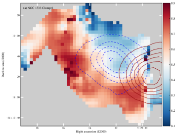
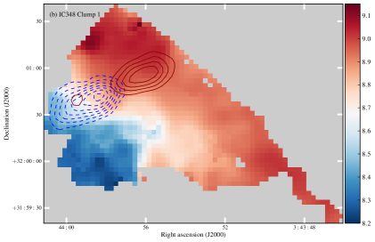
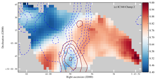
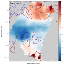
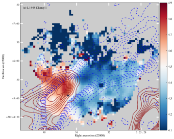
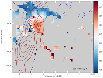
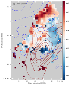
Figure 7: Outflow orientation compared to the velocity gradient direction for clumps in Table 5. The colour-scale is the C¹⁸O $J=3\to 2$ line centre in km s^-1 for map pixels allocated to each clump. Overlaid are contours of CO $J=3\to$ integrated antenna temperature $\int T_{\mathrm{A}}^{*}\mathrm{d}v$ for the blue- and red-shifted line wings, integrated from: $-5$ to 3 (blue) and 12 to 18 km s^-1 (red) for NGC 1333, $-5$ to 6 (blue) and 11 to 15 km s^-1 (red) for IC348 and $-5$ to 0 (blue) and 8 to 15 km s^-1 (red) for L1448. Contours are at various heights in K km s^-1 ($n$ is an integer from zero to $n_{\mathrm{max}}$): (a) (2+4$n$), $n_{\mathrm{max}}=4$ (blue) and (4+4$n$), $n_{\mathrm{max}}=6$ (red). (b) (6+2$n$), $n_{\mathrm{max}}=6$ (blue) and (6+2$n$), $n_{\mathrm{max}}=3$ (red). (c) (8+1.5$n$), $n_{\mathrm{max}}=6$ (blue) and (4+1.5$n$), $n_{\mathrm{max}}=8$ (red). (d) (5+$n$), $n_{\mathrm{max}}=4$ (blue) and (2+$n$), $n_{\mathrm{max}}=2$ (red). (e) (2+$n$), $n_{\mathrm{max}}=8$ (blue) and (2+2$n$), $n_{\mathrm{max}}=7$ (red). (f) (2+4$n$), $n_{\mathrm{max}}=5$ (both blue and red). (g) (2+4$n$), $n_{\mathrm{max}}=5$ (blue and red).

Thus, we must view the interpretation of a linear velocity gradient as unequivocal evidence of solid-body rotation with some scepticism. However, in the absence of a strong outflow i.e. for starless clumps and assuming we can consider each clump as a single object, rotation would seem to be a likely cause of a coherent velocity gradient and the only one we consider in the following analysis.

3.3.3 Fitted gradients

Table 6 lists the rates of detecting significant velocity gradients towards various core populations, separated by their different clump-finding algorithms, regions or types of source. They are similar for both algorithms with approximately a third of clumps displaying significant velocity gradients. The detection rate for Class 0 sources in the clfind catalogue is nearly twice as large as for the other types and Class 0s with gaussclumps. This is probably because Class 0 sources have typically stronger outflows than Class Is (e.g. Bontemps et al., 1996; Paper II). It is clear in Fig. 7 that many of the outflows extend beyond their associated clump. However, the clumps found by gaussclumps are smaller (Curtis & Richer, 2010) with a definite elliptical shape, which does not necessarily follow the orientation of the outflow. The lower detection rate for Class 0 sources with gaussclumps is perhaps another example of how their velocity gradients are dominated by outflows. If the smaller gaussclumps cores trace their shape less effectively, we would expect a lower detection rate.

Table 6: Number of clumps with significant velocity gradients by region, source type and algorithm. Percentages give the detection rate for the particular type of source in each region or overall.

Source Type	Region
	NGC 1333	IC348	L1448	Total
clfind Population
Starless	4(67 %)	2(17 %)	0(0 %)	6(32 %)
Class 0	7(64 %)	3(100 %)	3(75 %)	13(72 %)
Class I	4(44 %)	1(50 %)	0(0 %)	5(45 %)
No HFR07 ID	1(8 %)	1(17 %)	1(9 %)	3(11 %)
All	16(41 %)	7(30 %)	4(25 %)	27(35 %)
gaussclumps Population
Starless	4(50 %)	6(55 %)	0(0 %)	10(48 %)
Class 0	6(50 %)	1(33 %)	0(0 %)	7(35 %)
Class I	3(33 %)	0(0 %)	0(0 %)	3(35 %)
No HFR07 ID	11(31 %)	3(38 %)	1(6 %)	15(24 %)
All	24(37 %)	10(42 %)	1(4 %)	35(31 %)

Table 7: Average rotational properties derived from the velocity-gradient fitting for the clfind clump population. All the errors listed ($\sigma$) are errors on the mean and not sample deviations.

Population	Number	${\cal G}$	$\sigma_{\cal G}$	$\beta_{\mathrm{rot}}$	$\sigma_{\beta}$	$j$	$\sigma_{j}$
		(km s-1 pc-1)				(km s-1 pc)
All	27	5.7	0.5	0.014	0.003	0.0019	0.0002
NGC 1333	16	5.7	0.7	0.0040	0.0010	0.0017	0.0002
IC348	7	5.0	0.6	0.015	0.006	0.0017	0.0003
L1448	4	7	2	0.032	0.016	0.0032	0.0009
Starless	6	5.5	1.0	0.013	0.007	0.0021	0.0005
Protostars	19	5.8	0.7	0.008	0.003	0.0019	0.0003
Class 0	14	6.1	0.8	0.010	0.004	0.0021	0.0003
Class I	5	4.9	1.5	0.003	0.001	0.0011	0.0001

Table 8: Average rotational properties derived from the velocity-gradient fitting for the gaussclumps clump population. All the errors listed ($\sigma$) are errors on the mean and not sample deviations.

Population	Number	${\cal G}$	$\sigma_{\cal G}$	$\beta_{\mathrm{rot}}$	$\sigma_{\beta}$	$j$	$\sigma_{j}$
		(km s-1 pc-1)				(km s-1 pc)
All	35	6.9	0.6	0.013	0.004	0.00120	0.00014
NGC 1333	24	7.4	0.7	0.015	0.006	0.0012	0.0002
IC348	10	5.6	0.8	0.007	0.001	0.0011	0.0002
Starless	10	5.0	0.6	0.006	0.001	0.0010	0.0002
Protostars	10	7.0	1.0	0.009	0.004	0.0012	0.0002
Class 0	7	6.4	1.0	0.008	0.005	0.0012	0.0002
Class I	3	8	3	0.012	0.010	0.0012	0.0003

The fitted gradients are in the range 1.5 to 13.0 km s^-1 pc^-1 and 2.5 to 16.0 km s^-1 pc^-1 for clfind and gaussclumps respectively. We provide a summary of all the different rotational properties for different categories of clumps in Tables 7 and 8. Fig. 8 is a histogram of their magnitude by region. The distributions are qualitatively similar for the different regions with the usual uncertainty due to the small sample sizes; Kolmogorov-Smirnov (K-S) tests do not conclusively reject or confirm the hypothesis that each sample is drawn from the same population. On average across all the regions, the gradients are $\langle{\cal G}\rangle=(5.7\pm 0.5)$ km s^-1 pc^-1 for clfind and $\langle{\cal G}\rangle=(6.9\pm 0.6)$ km s^-1 pc^-1 for gaussclumps. The fitted gaussclumps gradients are larger than those for clfind but may be misleading as there are only 16 clumps with detections in both. We plot the gradient found with the clfind designation versus that with gaussclumps for these common sources in Fig. 9. There is fairly good agreement on the gradient with the protostellar sources deviating the most from the line of equal gradients. This might again be because the C¹⁸O line centres are affected by outflowing gas which is not well traced by the gaussclumps outlines.

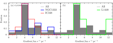
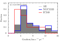
Figure 8: Distribution of significant ($\sigma_{\cal G}/{\cal G}\geq 3$) velocity gradients for the clfind (top) and gaussclumps (bottom) clump populations. The L1448 distribution is not plotted for gaussclumps as it has only one significant gradient.

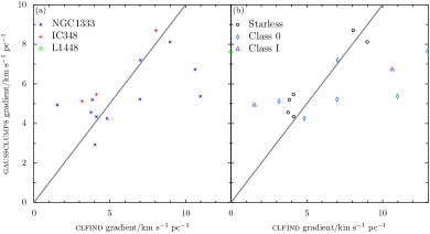
Figure 9: Fitted velocity gradient for gaussclumps versus clfind designations for the 16 clumps which have significant detections with both algorithms, by region (left) or by the classifications of HFR07 (right). The line marks where both gradients are equal.

There are too few sources of each classification to draw firm conclusions about any trends with age. It does seem in the distributions of Fig. 10 that the starless cores have ${\cal G}\la 10$ km s^-1 pc^-1 and larger gradients are protostellar. The protostellar average is larger than the starless one for the gaussclumps population: $\langle{\cal G}\rangle=(7.0\pm 1.0)$ compared to $\langle{\cal G}\rangle=(5.0\pm 0.6)$ km s^-1 pc^-1. Although they are similar for clfind $\langle{\cal G}\rangle=(5.8\pm 0.7)$ compared to $\langle{\cal G}\rangle=(5.5\pm 1.0)$ km s^-1 pc^-1. This might point to an outflow contribution to the gradient.

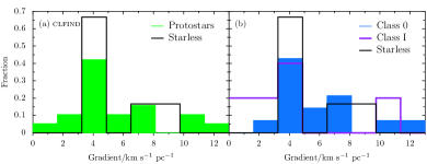
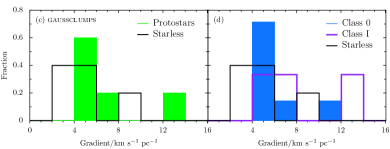
Figure 10: Distribution of significant ($\sigma_{\cal G}/{\cal G}\geq 3$) velocity gradients for the classifications of HFR07 for the clfind (top) and gaussclumps (bottom) clump populations.

The gradients we find in Perseus are much greater than those originally found by GBF93 or Caselli et al. (2002) in their N₂H⁺ $J=1\to 0$ survey of 60 low mass cores: 0.3 to 3.9 and 0.5 to 6.0 km s^-1 pc^-1 respectively. Outflows cannot explain all of this difference because our starless clumps have significantly larger gradients as well. The discrepancy is reminiscent of that found by GBF93 towards B361, which was also investigated by Arquilla & Goldsmith (1985) with ¹³CO $J=1\to 0$ data. GBF93 estimated a gradient five times smaller than the earlier study, 0.7 versus 3.3 km s^-1 pc^-1, which had led Arquilla & Goldsmith (1985) to conclude that rotation was dynamically significant in dark clouds. GBF93 explain the difference by emphasizing that tracers of lower critical densities can produce complicated velocity patterns dominated by outflows or clump-to-clump motions that mimic solid body rotation. However, Olmi, Testi & Sargent (2005) fitted gradients to a number of cores in Perseus, finding similar magnitudes for the two common cores also in GBF93 and generally in the same range 0.14 to 2.32 km s^-1 pc^-1. Their study used C¹⁸O $J=1\to 0$, CS $J=2\to 1$ and N₂H⁺ $J=1\to 0$ data with their C¹⁸O fitting not displaying markedly different gradients. A critical factor will undoubtedly be resolution. The angular resolution of previous surveys is worse than the 17.7 arcsec of our maps: $\sim$88, $\sim$54 and $\sim$46 arcsec for GBF93, Caselli et al. (2002) and Olmi et al. (2005) respectively. Hence even for their closest sources in Taurus (at 140 pc), their best linear resolution (0.037 pc) is nearly twice as large as ours (0.021 pc). A larger beam will tend to smooth out differences between regions and reduce the overall gradient magnitude. This effect may be large enough to explain the differences for cores perhaps three times as distant as Perseus, in a beam four times as large as ours.

3.3.4 Gradient orientation

Centrifugal stresses due to energetic rotation will flatten cores along the rotation axis. This tends to produced oblate cores (GBF93), currently the favoured shape (e.g. Jones, Basu & Dubinski 2001), which could also be caused by strong magnetic fields. If rotation dominates, we might expect the the degree of core elongation to increase with increasing velocity gradient and a core’s major axis to lie parallel to the gradient i.e. perpendicular to the rotation axis. Fig. 11 shows no relationship between the magnitude of the velocity gradient and the elongation of a clump, quantified through the axis ratio (taken from Curtis & Richer 2010). It comes as no surprise then that the angle between the clump major axis and the velocity gradient in Fig. 12 (only computed for the gaussclumps sources), seems to be distributed at random as well. Therefore, clump rotation is unlikely to be energetically significant.

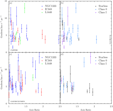
Figure 11: Velocity gradient versus axis ratio for clfind (top panels) and gaussclumps sources (bottom panels) broken down by region (left panels) or by the classifications of HFR07 (right panels).

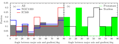
Figure 12: Distribution of the angle between the velocity gradient and the major axis of the gaussclumps clumps by region (left) or by the classifications of HFR07 (right). If rotational motions are elongating the clumps we would expect the gradient and axis to be in the same direction making the angle zero.

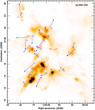
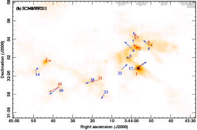
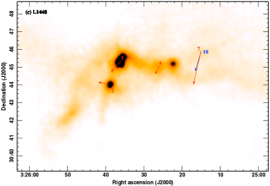
Figure 13: Spatial distribution of the velocity gradient detections in NGC 1333 (top), IC348/HH211 (middle) and L1448 (bottom). Arrows are drawn from the peak position of the associated clump for clumps where there are significant detections in either the clfind or gaussclumps catalogues. The direction and length of the arrow represents the direction and magnitude of the gradient and the detections are labelled with the reference from our SCUBA catalogues (Curtis & Richer, 2010). The colour-scale is SCUBA 850 µm emission from 0 to 1600 mJy beam^-1.

Is there a correlation between the orientation of the rotation axes of neighbouring clumps or an anti-correlation to keep the net angular momentum small? In Fig. 13, we overlay the velocity gradients on dust emission maps of the various regions. Reassuringly the directions and magnitudes of the gradients measured using both algorithms’ allocations match very well. In small patches the arrows of neighbouring clumps line up but on large scales there seems to be little correlation. This is similar to the gravoturbulent models of JK04, where shortly after collapse starts, the angular momenta in small regions are well aligned over a moderate correlation length with cores further away spinning in random directions. Their explanation is that neighbouring cores are formed from the same reservoir of material and therefore can be expected to have similar angular momenta. During subsequent accretion and evolution, the associated correlation length decreases and neighbours lose their alignment, as embedded cores are ejected and turbulence disrupts the current material or brings in new gas.

3.3.5 Dynamic support?

To quantify the level of support that the velocity gradients might provide against gravitational collapse we calculate $\beta_{\mathrm{rot}}$, the ratio of rotational to gravitational energy. GBF93 define this ratio for a uniform density sphere:

$$\beta_{\mathrm{rot}}=\frac{(1/2)I\omega^{2}}{3GM^{2}/5R}=\frac{R^{3}{\cal G}^{2}}{3GM\sin^{2}i}$$ (8)

where the moment of inertia is $I=pMR^{2}$ with $p=2/5$ for a uniform density sphere and the angular momentum is $\omega={\cal G}/\sin i$ with $i$ the angle of inclination to the line of sight. Assuming values representative of these clumps and $\sin i=1$, this becomes:

$$\beta_{\mathrm{rot}}=6.2\times 10^{-4}\left(\frac{R_{\mathrm{dec}}}{0.02\,\mathrm{pc}}\right)^{3}\left(\frac{M}{\mathrm{M_{\odot}}}\right)^{-1}\left(\frac{{\cal G}}{\mathrm{1\,km\,s^{-1}\,pc^{-1}}}\right)^{2}.$$ (9)

Across all the clumps the average values of $\beta_{\mathrm{rot}}$ are: $\langle\beta_{\mathrm{rot}}\rangle=(0.014\pm 0.003)$ and $(0.013\pm 0.004)$ for clfind and gaussclumps respectively. At most the rotational energy is just six per cent for the clfind sample and 14 per cent for gaussclumps of the gravitational energy in the clumps. Fig. 14 shows the distribution of $\beta_{\mathrm{rot}}$ for the two clump populations. There is a strong preference for low ratios, with the fraction of clumps rapidly falling off as $\beta_{\mathrm{rot}}$ increases. Additionally, both populations closely match each other and the ratios found by Caselli et al. (2002), while the GBF93 distribution is wider, spreading to higher values. K-S tests could not confirm the samples are drawn from the same population as each other or either of the examples from the literature to any degree of significance. Even though we found larger velocity gradients than the previous studies, $\beta_{\mathrm{rot}}$ is not any higher. This is probably because our clumps are significantly smaller: on average the clump radii are 0.03 and 0.02 pc for clfind and gaussclumps respectively while the Caselli et al. (2002) cores have an average of 0.06 pc. As $\beta_{\mathrm{rot}}$ depends on $R^{3}$ this will reduce our values by $\sim$9 relative to theirs for an equally massive source, compensating for our larger derived gradients. Thus, rotation is not dynamically significant in star-forming cores and should not support the core against collapse.

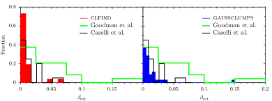
Figure 14: Distribution of the ratio of rotational to gravitational energies, $\beta_{\mathrm{rot}}$. For comparison the distributions found by GBF93 (green) and (Caselli et al. 2002, orange) are overlaid.

It would be interesting to examine how the level of support varies region-to-region and as a clump evolves. However, the numbers here are too small to draw any firm conclusions, with one or two objects heavily distorting overall averages. This is further compounded by the outflow ambiguities of the protostellar sources. Nevertheless, there are no vast differences in the populations by region or age with almost all the clumps having $\beta_{\mathrm{rot}}\la 0.02$.

3.3.6 Angular momenta

The core rotation speed can be quantified via the specific angular momentum, $j=J/M$, i.e. the angular momentum per unit mass:

$$j=\frac{2}{5}\omega R^{2}$$ (10)

where $\omega={\cal G}/\sin i$ is again the angular velocity of the clump, $R$ its radius and the factor $2/5$ is for a constant density sphere. This yields for representative values:

$$j=1.6\times 10^{-4}\left(\frac{\cal G}{1\,\mathrm{km\,s^{-1}\,pc^{-1}}}\right)\left(\frac{R_{\mathrm{dec}}}{0.02\,\mathrm{pc}}\right)^{2}\,\mathrm{km\,s^{-1}\,pc}$$ (11)

The distribution of $j$ has been important, with modellers using the one derived by GBF93 either as an input to their models or a target (e.g. Burkert & Bodenheimer, 2000; JK04). Furthermore, the distribution of angular momentum across a core and its evolution may prove whether magnetic fields are necessary to strip off angular momentum as collapse ensues.

In Fig. 15, we plot the distribution of $j$ by region. There is little difference between the different algorithms or clumps from one region to the next. For clfind the overall average is $\langle j\rangle=(1.9\pm 0.2)\times 10^{-3}$ km s^-1 pc whilst $\langle j\rangle=(1.7\pm 0.2)\times 10^{-3}$, $(1.7\pm 0.3)\times 10^{-3}$ and $(3.2\pm 0.9)\times 10^{-3}$ in NGC 1333, IC348 and L1448 respectively. The gaussclumps data are skewed to lower $j$ due to their smaller clump radii but there are still few differences across the regions: $\langle j\rangle=(1.20\pm 0.14)\times 10^{-3}$, $(1.2\pm 0.2)\times 10^{-3}$, $(1.1\pm 0.2)\times 10^{-3}$ km s^-1 pc overall and in NGC 1333 and IC348 respectively.

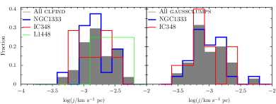
Figure 15: Distribution of $j$ by region and algorithm: clfind on the left and gaussclumps on the right.

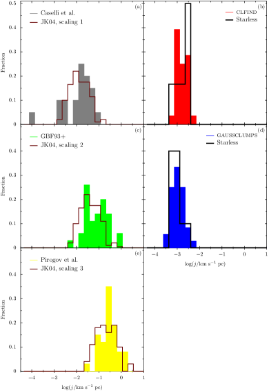
Figure 16: Distribution of specific angular momenta, $j$ for starless cores. (a) N₂H⁺ $J=1\to 0$ cores of Caselli et al. (2002, grey) compared to the JK04 model (brown) scaled by $n=10^{5}$ cm^-3 and $T=10$ K. (b) All our clfind detections (red) and just those in starless clumps (black). (c) NH₃ cores of GBF93, Barranco & Goodman (1998) and Jijina et al. (1999) (green) compared to the JK04 model (brown) scaled by $n=10^{4}$ cm^-3 and $T=10$ K. (d) all our gaussclumps detections (blue) and just those in starless clumps (black). (e) N₂H⁺ $J=1\to 0$ high-mass cores of Pirogov et al. (2003) compared to the JK04 model (brown) scaled by $n=10^{4}$ c ^-3 and $T=50$ K.

JK04 distinguish between starless and protostellar sources in their gravoturbulent simulations which focus particularly on rotational properties. They find wide continuous distributions for $j$, stretching over two orders of magnitude, as we do. Their prestellar cores have an order of magnitude larger $j$ than the protostars. Fig. 16 compares our distributions of $j$ (overall and for the starless clumps) to previously observed distributions and JK04. To match a particular set of observations, JK04 scale their code output according to the mean density, $n$, and temperature, $T$, with $j$ depending on these as $j\propto T/\sqrt{n}$. With appropriate scalings their data match three different observational regimes: low-mass cores mapped in the high-density tracer N₂H⁺ (Caselli et al., 2002), low-mass cores in the slightly lower density tracer NH₃ (GBF93 with Barranco & Goodman, 1998 and Jijina, Myers & Adams, 1999) and high-mass cores in the high-density tracer N₂H⁺ (Pirogov et al., 2003). Our observed distribution has no overlap with the high-mass cores of Pirogov et al. (2003) and little with GBF93, having much lower $j$. For the starless clumps only, we find $\langle j\rangle=(2.1\pm 0.5)\times 10^{-3}$ and $(1.0\pm 0.2)\times 10^{-3}$ km s^-1 pc for clfind and gaussclumps respectively. The most similar distribution is that of Caselli et al. (2002), which is over twice as wide with a much larger average, $\langle j\rangle=2.2\times 10^{-2}$ km s^-1 pc, but does overlap with ours at low $j$. For our average to match that of Caselli et al. (2002), presumably our clumps would have to be considerably denser and/or colder than the values assumed by JK04 of $n=10^{5}$ cm^-3 and $T=10$ K. In §3 we noted that the critical density is expected to be $n_{\mathrm{crit}}=10^{4}$ cm^-3. However, in radiative transfer models of a free-falling protostellar envelope, we found peak H₂ number densities of greater than a few times $10^{5}$ cm^-3 were required to reproduce the C¹⁸O $J=3\to 2$ line strengths seen in our data (Curtis, 2009). Alternatively or additionally, we are seeing considerably smaller angular momenta then those measured by previous authors. The narrow width of the distribution compared to previous work is likely to reflect the uniform environment of our cores in a single cloud rather then spread over many different ones as in Caselli et al. (2002) and GBF93.

On the other hand, the smaller angular momenta observed in our starless clumps may not indicate lower degrees of rotation in the clump core but may reflect a more slowly rotating outer envelope, making comparisons with tracers such as NH₃ inappropriate. Redman et al. (2004) examined the asymmetric HCO⁺ line profiles across L1689B, a prestellar core in Ophiuchus, which they modelled as a rapidly-rotating inner core contained within a static envelope. Again, the key diagnostics are the densities and temperatures traced by the C¹⁸O $J=3\to 2$ line, which can only be properly answered with radiative transfer modelling. We would expect to probe high densities, $n_{\mathrm{crit}}\sim 10^{4}$ cm^-3, but earlier we saw the similar non-thermal linewidths for the $J=3\to 2$ line compared to the $J=2\to 1$, suggesting we might not be detecting very different material. A further consideration in the low temperature environments of starless cores is CO depletion. Estimating the degree of depletion in these cores is difficult without similar observations in “late-depleting” molecules, such as N₂H⁺. However, models (e.g. Walmsley, Flower & Pineau des Forêts, 2004) suggest that CO freezes-out in the central 7000 AU of a prestellar core (this is really a temperature and density dependence). Furthermore, we noted in §3.1 that there is some existing evidence for considerable C¹⁸O depletion in candidate star-forming cores in Perseus (KJT07) Thus, our C¹⁸O signal in evolved starless clumps and young protostars at least should have little contribution from the dense inner core and this reasoning supports the idea we are probing a more slowly rotating envelope.

In JK04, protostars have a distribution of $j$ that narrows with time, staying around the same average. Their distribution is also similar to that observed for binaries (see Fig. 17). Our distributions for all the sources are as narrow as those for the protostars alone in JK04’s models. For clfind there is a trend of decreasing $j$ with protostellar age: $\langle j\rangle=(2.1\pm 0.3)\times 10^{-3}$ and $(1.1\pm 0.1)\times 10^{-3}$ km s^-1 pc for Class 0 and I clumps, which is not reproduced with gaussclumps: $\langle j\rangle=(1.2\pm 0.2)\times 10^{-3}$ (Class 0) and $(1.2\pm 0.3)\times 10^{-3}$ km s^-1 pc (Class I). Of course in these sources there is potential confusion of the rotational signatures with outflows which is perhaps why the expected decrease in $j$ from starless to protostellar clumps is not observed.

Figure 17: Distribution of the specific angular momenta, $j$, for protostars. (a) to (d) show JK04’s model M6k2 with different star formation efficiencies: (a) 15, (b) 30, (c) 45 and (d) 60 per cent. (e) Binaries among nearby G stars of Duquennoy & Mayor (1991). (f) Binaries in Taurus (Simon, 1992). (g) and (h) show the distributions from paper for the clfind and gaussclumps designations respectively, decomposed according to the designations of HFR07.

3.3.7 Scalings with clump size

GBF93 found that many of the derived rotation parameters scale with radius, including ${\cal G}$ ($\propto R^{-0.4}$) and $j$ ($\propto R^{1.6}$) but not $\beta_{\mathrm{rot}}$. We plot the same parameters as a function of clump size in Fig. 18. Most of the relations found by GBF93 hold for these clumps, although there is considerable scatter. GBF93 show that the relation for the gradient is implied from a linewidth-size relation (e.g. Larson, 1981), $\Delta v=R^{0.6}$, for a core in virial equilibrium. we find $\beta_{\mathrm{rot}}$ is independent of $R$ as well, implying $M\propto R^{3}$ for solid body rotation ($\omega=$ constant) or for differential rotation ($\omega\propto R^{-1}$) that $M\propto R$. The SCUBA clumps follow $M\propto R^{2}$ (Curtis & Richer, 2010), so we can infer a more complicated form of rotation than pure solid body or differential to ensure $\beta_{\mathrm{rot}}$ is independent of size.

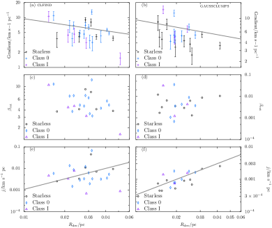
Figure 18: Rotational parameters as functions of clump size for clfind (left) and gaussclumps (right). ${\cal G}$ versus clump radius; $\beta_{\mathrm{rot}}$ versus $R_{\mathrm{dec}}$ (middle panels); $j$ versus $R_{\mathrm{dec}}$ (bottom panels). Lines mark the GBF93 relations: ${\cal G}\propto R^{-0.4}$ and $j\propto R^{1.6}$.

The scaling of $j$ with size is of particular interest. Ohashi et al. (1997) looked at rotation in protostars in Taurus using C¹⁸O $J=1\to 0$ interferometric spectra. They found at distances $\la 3500$ AU, that $j$ was at a constant value of $\sim$10^-3 km s^-1 pc. These findings are consistent with magnetically-controlled collapse elucidated by Belloche et al. (2002), where in a dense inner core, the angular momentum is locked at a minimum value. This region could be interpreted as a magnetically supercritical core, decoupling from its subcritical environment, where $j$ scales with $R$. In our data a horizontal line is almost as convincing as the slope of GBF93, indeed the spread of clump sizes is not really wide enough to constrain the trend unambiguously. Our results are therefore consistent with this magnetically-controlled scenario: there is a lot of spread about $j\sim$10^-3 km s^-1 pc but no $j$ much below this value. How the rotational velocity changes across a clump is less clear and is a key discriminator between different theories. Such measurements would require high-resolution, interferometric observations of many cores in different stages of collapse.

4 Summary

We have analysed the kinematic signatures of two populations of dust continuum clumps identified in SCUBA 850 µm data using either clfind or gaussclumps (Curtis & Richer, 2010), across four regions (NGC 1333, IC348/HH211, L1448 and L1455) of active star formation in the Perseus molecular cloud. The kinematics were derived from our large-scale (600 arcmin²) C¹⁸O $J=3\to 2$ survey (Paper I). First, the non-thermal contribution to the C¹⁸O linewidth was calculated and compared to the results of KJT07 and the gravoturbulent models of Klessen et al. (2005):

1. Most clumps have supersonic non-thermal linewidths, $\langle\sigma_{\mathrm{NT}}/c_{\mathrm{s}}\rangle=1.76\pm 0.09$ (clfind population) or $1.71\pm 0.05$ (gaussclumps), with overall distributions similar to the C¹⁸O $J=2\to 1$ data of KJT07 towards dense core candidates in Perseus. This implies we are also probing the ‘envelopes’ of the star-forming clumps rather than deep within their interiors.

2. There is little difference in the level of the non-thermal linewidth contribution between protostars and starless clumps, implying that protostars do no affect their environment significantly. Clumps in NGC 1333 and IC348 are in the vicinity of young stellar clusters, explaining the wider linewidths in NGC 1333 ($\langle\sigma_{\mathrm{NT}}/c_{\mathrm{s}}\rangle=1.91\pm 0.07$) than L1448 ($1.52\pm 0.13$) for the gaussclumps objects (although their linewidths are similar for clfind population: $2.05\pm 0.12$ and $1.8\pm 0.2$ respectively). IC348 however, has the narrowest lines of all ($1.36\pm 0.09$ with clfind and with $1.44\pm 0.07$ gaussclumps), possibly related to its statistically younger population (Hatchell et al., 2005), containing more starless clumps.

Second, the C¹⁸O linewidths allowed an estimate of each clump’s virial mass:

1. Most clumps in Perseus appear bound and close to equipartition. The ratio of the SCUBA to virial mass for clumps based on flux allocation using clfind is $\langle M_{850}/M_{\mathrm{vir}}\rangle=1.32\pm 0.13$, compared to $0.9\pm 0.1$ for the gaussclumps decomposition.

2. Starless clumps occupy a similar section of $M_{850}$-$M_{\mathrm{vir}}$ parameter space to the protostars suggesting that they are gravitationally bound and therefore truly prestellar. This has implications for our previous work investigating the starless CMF in Perseus (Curtis & Richer, 2010).

These results are in contrast to the models of Klessen et al. (2005) where a majority of starless core have $M_{\mathrm{vir}}\gg M$ and occupy a different parameter space to the protostars.

Finally, we fitted a linear velocity gradient to the C¹⁸O line centres, across the face of each SCUBA clump, again identified either with clfind or gaussclumps. Significant detections were found in approximately a third of the clumps, which we interpreted in terms of solid-body rotation.

1. A correlation between CO $J=3\to 2$ outflows and the C¹⁸O line centres is observed, implying any gradients in outflow sources, i.e. protostars, may reflect outflows rather than rotation.

2. The fitted gradients, in the range $\sim 1$ to 16 km s^-1 pc^-1, are larger than those previously observed. This probably results from the higher angular resolution of our observations and/or outflow contamination.

3. There is no correlation between the gradient direction and the clump orientation nor between the gradient and clump axis ratio, implying that the rotation is not energetically significant. Furthermore, the ratio of the clump rotational to gravitational energy is typically $\la 0.02$, demonstrating that rotation is not dynamically important as well, with a distribution very similar to that of the N₂H⁺ cores of Caselli et al. (2002).

4. The distribution of specific angular momentum is narrower and centred around lower values, $j\sim 10^{-3}$ km s^-1 pc, than previous studies. Interpreting the results of JK04 this suggests a denser and/or colder environment for the Perseus clumps than seen in the Caselli et al. (2002) sample (taken to have $n\sim 10^{5}$ cm^-3 and $T\sim 10$ K). This would seem unlikely given the large linewidths we observed towards the clumps, although radiative transfer modelling does suggest we are probing moderately high densities – peak H₂ number densities of a few $\times 10^{5}$ cm^-3 for a free-falling protostellar envelope (Curtis, 2009). Thus, we are probably seeing lower levels of rotation in our clumps.

5. There are no strong trends in the rotational parameters with radius.

The somewhat inconclusive findings of this paper motivate further work on the star-forming cores in Perseus. First, the construction of accurate radiative transfer models to determine precisely the conditions traced by the CO $J=3\to 2$ transitions. Second, higher-resolution or higher-tracer-density observations. $j$ found in our clumps, suggestively hovers around the background value, $10^{-3}$ km s^-1 pc^-1, found by Ohashi et al. (1997) at radii $\lesssim 0.03$ pc in Taurus’s protostellar cores. To see how exactly $j$ varies with radius we need to probe across the clumps themselves, using higher-density tracers or higher-resolution observations.

5 Acknowledgments

EIC thanks the Science and Technology Facilities Council (STFC) for studentship support while carrying out this work. We thank Jane Buckle and Gary Fuller for reading carefully an early version of this paper. We are grateful to the referee, for comments and suggestions which improved the clarity of this paper. The JCMT is operated by The Joint Astronomy Centre (JAC) on behalf of the STFC of the United Kingdom, the Netherlands Organisation for Scientific Research and the National Research Council (NRC) of Canada. We have also made extensive use of the SIMBAD data base, operated at CDS, Strasbourg, France. We acknowledge the data analysis facilities provided by the Starlink Project which is maintained by JAC with support from STFC. This research used the facilities of the Canadian Astronomy Data Centre operated by the NRC with the support of the Canadian Space Agency.

Appendix A Derived core dynamical and rotational properties

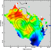
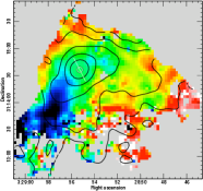
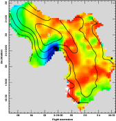
NGC 1333 2	NGC 1333 3	NGC 1333 5

Figure 19: SCUBA 850 µm clumps identified with clfind containing significant velocity gradients, $\sigma_{\cal G}/{\cal G}\geq 3$ in NGC 1333, IC348 and L1448. The colour-scale denotes the C¹⁸O $J=3\to 2$ line centre velocity, linearly scaled from the clump minimum (blue/black) to maximum (red/white). Contours of 850 $\mu$m flux density are overlaid (black) at 100, 200, 400, 800, 1600 and 3200 mJy beam^-1. A white/black circle marks the position of the clump peak emission with a white line positioned to show the direction of the fitted velocity gradient. The full version of this figure is available as Supporting Information to the online version of this article.

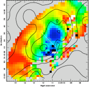
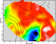
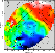
NGC 1333 1	NGC 1333 4	NGC 1333 7

Figure 20: SCUBA 850 µm clumps identified with gaussclumps containing significant velocity gradients, $\sigma_{\cal G}/{\cal G}\geq 3$ in NGC1333, IC348 and L1448. The colour-scale denotes the C¹⁸O $J=3\to 2$ line centre velocity, linearly scaled from the clump minimum (blue/black) to maximum (red/white). Contours of 850 $\mu$m flux density are overlaid (black) at 100, 200, 400, 800, 1600 and 3200 mJy beam^-1. A white/black circle marks the position of the clump peak emission with a white line positioned to show the direction of the fitted velocity gradient. The full version of this figure is available as Supporting Information to the online version of this article.

We list linewidths, virial masses and rotational parameters alongside other properties for every clump examined in Tables 9, 10, 11 and 12. In Figs. 19 and 20, we plot the C¹⁸O $J=3\to 2$ line centre velocity and best-fitting velocity gradient for every SCUBA clump with a significant detection.

Table 9: Dynamical properties of SCUBA clumps found with clfind. The full version of this table is available as Supporting Information to the online version of this article.

Sub-region a	Clump b	Hatchell c	$T_{\mathrm{NH_{3}}}$ d	$v_{\mathrm{c}}(\mathrm{C^{18}O})$ e	$\Delta v_{\mathrm{C^{18}O}}$ f	$\sigma_{\mathrm{NT}}$ g	$M_{\mathrm{vir}}$ h
	ID	ID	(K)	(km s-1)	(km s-1)	(km s-1)	(M⊙)
NGC 1333	1	42	13.5	7.36	1.91	0.81	11.3
NGC 1333	2	43	16.3	8.24	1.53	0.64	11.9
NGC 1333	3	44	16.5	7.62	1.19	0.50	12.3
NGC 1333	4	41	15.0	7.48	1.81	0.77	13.7
NGC 1333	5	45	16.4	7.79	1.40	0.59	22.9
…

^a Name of sub-region map.

^b Clump number from Curtis & Richer (2010).

^c H07 identifier.

^d Rosolowsky et al. (2008) NH₃ kinetic temperature where they exist or 10.0, 15.0 and 12.0 K for starless clumps, protostars and clumps with no H07 identification where not respectively.

^e,f Measured C¹⁸O $J=3\to 2$ line centre velocity, $v_{\mathrm{c}}$ and FWHM, $\Delta v_{\mathrm{C^{18}O}}$ from a Gaussian fit to the line profile at the clump peak.

^g Non-thermal contribution to the linewidth estimated using the temperatures of column (d).

^h Virial masses calculated using the temperatures of column (d).

Table 10: Dynamical properties of SCUBA clumps found with gaussclumps. The full version of this table is available as Supporting Information to the online version of this article.

Sub-region a	Clump b	Hatchell c	$T_{\mathrm{NH_{3}}}$ d	$v_{\mathrm{c}}(\mathrm{C^{18}O})$ e	$\Delta v_{\mathrm{C^{18}O}}$ f	$\sigma_{\mathrm{NT}}$ g	$M_{\mathrm{vir}}$ h
	ID	ID	(K)	(km s-1)	(km s-1)	(km s-1)	(M⊙)
NGC 1333	1	41,42	15.0	6.77	1.04	0.44	11.9
NGC 1333	2	43	16.3	8.18	1.51	0.64	5.8
NGC 1333	3	–	16.5	7.62	1.19	0.50
NGC 1333	4	45	16.4	7.82	1.35	0.57	8.7
NGC 1333	5	46	14.3	8.40	1.27	0.54	4.0
…

^a Name of sub-region map.

^b Clump number from Curtis & Richer (2010).

^c H07 identifier.

^d Rosolowsky et al. (2008) NH₃ kinetic temperature where they exist or 10.0, 15.0 and 12.0 K for starless clumps, protostars and clumps with no H07 identification where not respectively.

^e,f Measured C¹⁸O $J=3\to 2$ line centre velocity, $v_{\mathrm{c}}$ and FWHM, $\Delta v_{\mathrm{C^{18}O}}$ from a Gaussian fit to the line profile at the clump peak.

^g Non-thermal contribution to the linewidth estimated using the temperatures of column (d).

^h Virial masses calculated using the temperatures of column (d).

Table 11: Rotational properties of SCUBA clumps located with clfind. These properties have been found by non-linear least squares fitting of a linear velocity gradient to the first moment of the C¹⁸O $J=3\to 2$ data. Only significant detections are shown with $\sigma_{\cal G}/{\cal G}\geq 3$. The full version of this table is available as Supporting Information to the online version of this article.

Sub-region a	Clump b	Hatchell c	Number d	${\cal G}\pm\sigma_{\cal G}$ e	$\theta_{\cal G}$ f	${\cal G}/\sigma_{\cal G}$ g	$\beta_{\mathrm{rot}}$ h	$j$ i
	ID	class	of points	(km s-1 pc-1)	(deg E of N)			(km s-1 pc)
NGC1333	2	I	1117	$3.16\pm 0.76$	155.44	4	6.98E-04	1.05E-03
NGC1333	3	0	2106	$4.85\pm 0.35$	26.88	14	5.39E-03	3.51E-03
NGC1333	5	I	2229	$1.54\pm 0.41$	21.10	4	8.91E-04	1.63E-03
NGC1333	6	0	978	$4.66\pm 0.84$	125.79	6	3.35E-03	1.44E-03
NGC1333	8	I	330	$10.63\pm 2.67$	-58.59	4	4.67E-03	9.83E-04
…

^a Name of sub-region map.

^b Clump identification from Curtis & Richer (2010).

^c H07 clump class, S=starless, 0=Class 0 protostar and I=Class I protostar. ^d Number of points fitted in the map.

^e Fitted velocity gradient and its error.

^f Angle of the fitted velocity gradient, east of north.

^g Level of significance of the fit, $\sigma_{\cal G}/{\cal G}$.

^h Ratio of the kinetic to gravitational energy.

ⁱ Specific angular momentum.

Table 12: Rotational properties of SCUBA clumps located with gaussclumps. These properties have been found by non-linear least squares fitting of a linear velocity gradient to the first moment of the C¹⁸O $J=3\to 2$ data. Only significant detections are shown with $\sigma_{\cal G}/{\cal G}\geq 3$. The full version of this table is available as Supporting Information to the online version of this article.

Sub-region a	Clump b	Hatchell c	Number d	${\cal G}\pm\sigma_{\cal G}$ e	$\theta_{\cal G}$ f	${\cal G}/\sigma_{\cal G}$ g	$\beta_{\mathrm{rot}}$ h	$j$ i
	ID	class	of points	(km s-1 pc-1)	(deg E of N)			(km s-1 pc)
NGC1333	1	0	800	$5.33\pm 1.33$	135.67	4	6.90E-04	7.86E-04
NGC1333	4	I	922	$4.93\pm 1.16$	-79.61	4	1.22E-03	7.41E-04
NGC1333	7	I	1222	$6.73\pm 0.84$	-77.95	8	4.27E-03	1.56E-03
NGC1333	8	0	812	$4.25\pm 1.11$	26.44	4	1.07E-03	5.54E-04
NGC1333	9	0	1374	$5.37\pm 0.65$	-38.35	8	3.70E-03	1.63E-03
…

^a Name of sub-region map.

^b Clump identification from Curtis & Richer (2010).

^c H07 clump class, S=starless, 0=Class 0 protostar and I=Class I protostar. ^d Number of points fitted in the map.

^e Fitted velocity gradient and its error.

^f Angle of the fitted velocity gradient, east of north.

^g Level of significance of the fit, $\sigma_{\cal G}/{\cal G}$.

^h Ratio of the kinetic to gravitational energy.

ⁱ Specific angular momentum.

References

- Alves et al. (2007) Alves J., Lombardi M., Lada C. J., 2007, A&A, 462, L17
- André et al. (2007) André P., Belloche A., Motte F., Peretto N., 2007, A&A, 472, 519
- Arquilla & Goldsmith (1985) Arquilla R., Goldsmith P. F., 1985, ApJ, 297, 436
- Ballesteros-Paredes et al. (2003) Ballesteros-Paredes J., Klessen R. S., Vázquez-Semadeni E., 2003, ApJ, 592, 188
- Barranco & Goodman (1998) Barranco J. A., Goodman A. A., 1998, ApJ, 504, 207
- Bate & Bonnell (2005) Bate M. R., Bonnell I. A., 2005, MNRAS, 356, 1201
- Belloche et al. (2002) Belloche A., André P., Despois D., Blinder S., 2002, A&A, 393, 927
- Benson & Myers (1989) Benson P. J., Myers P. C., 1989, ApJS, 71, 89
- Bertoldi & McKee (1992) Bertoldi F., McKee C. F., 1992, ApJ, 395, 140
- Binney & Tremaine (2008) Binney J., Tremaine S., 2008, Galactic Dynamics. Princeton Univ. Press, Princeton, NJ
- Bonnell et al. (2001) Bonnell I. A., Bate M. R., Clarke C. J., Pringle J. E., 2001, MNRAS, 323, 785
- Bontemps et al. (1996) Bontemps S., Andre P., Terebey S., Cabrit S., 1996, A&A, 311, 858
- Buckle et al. (2009) Buckle J. V., et al., 2009, MNRAS, 399, 1026
- Buckle et al. (2010) Buckle J. V., et al., 2010, MNRAS, 401, 204
- Burkert & Bodenheimer (2000) Burkert A., Bodenheimer P., 2000, ApJ, 543, 822
- Caselli & Myers (1995) Caselli P., Myers P. C., 1995, ApJ, 446, 665
- Caselli et al. (2002) Caselli P., Benson P. J., Myers P. C., Tafalla M., 2002, ApJ, 572, 238
- Clark et al. (2007) Clark P. C., Klessen R. S., Bonnell I. A., 2007, MNRAS, 379, 57
- Curtis (2009) Curtis E. I., 2009, PhD thesis, Univ. of Cambridge
- Curtis & Richer (2010) Curtis E. I., Richer J. S., 2010, MNRAS, 402, 603
- Curtis et al. (2010a) Curtis E. I., Richer J. S., Buckle J. V., 2010a, MNRAS, 401, 455 (Paper I)
- Curtis et al. (2010b) Curtis E. I., Richer J. S., Swift J. J., Williams J. P., 2010b, MNRAS, in press (Paper II)
- Dib et al. (2007) Dib S., Kim J., Vázquez-Semadeni E., Burkert A., Shadmehri M., 2007, ApJ, 661, 262
- Dib et al. (2010) Dib S., Hennebelle P., Pineda J. E., Csengeri T., Bontemps S., Audit E., Goodman A. A., 2010, ApJ, in press
- Duquennoy & Mayor (1991) Duquennoy A., Mayor M., 1991, A&A, 248, 485
- Elmegreen et al. (2000) Elmegreen B. G., Efremov Y., Pudritz R. E., Zinnecker H., 2000, in Mannings V., Boss A. P., Russell S. S., eds, Protostars and Planets IV. Univ. of Arizona Press, Tucson, p. 179
- Elmegreen & Scalo (2004) Elmegreen B. G., Scalo J., 2004, ARA&A, 42, 211
- Enoch et al. (2006) Enoch M. L., et al., 2006, ApJ, 638, 293
- Enoch et al. (2008) Enoch M. L., Evans II N. J., Sargent A. I., Glenn J., Rosolowsky E., Myers P., 2008, ApJ, 684, 1240
- Galli et al. (2002) Galli D., Walmsley M., Gonçalves J., 2002, A&A, 394, 275
- Gammie et al. (2003) Gammie C. F., Lin Y.-T., Stone J. M., Ostriker E. C., 2003, ApJ, 592, 203
- Goodman et al. (1993) Goodman A. A., Benson P. J., Fuller G. A., Myers P. C., 1993, ApJ, 406, 528 (GBF93)
- Goodman et al. (1998) Goodman A. A., Barranco J. A., Wilner D. J., Heyer M. H., 1998, ApJ, 504, 223
- Goodwin & Kouwenhoven (2009) Goodwin S. P., Kouwenhoven M. B. N., 2009, MNRAS, 397, L36
- Goodwin et al. (2007) Goodwin S. P., Kroupa P., Goodman A., Burkert A., 2007, in Reipurth B., Jewitt D., Keil K., eds, Protostars and Planets V. Univ. of Arizona Press, Tucson, p. 133
- Goodwin et al. (2008) Goodwin S. P., Nutter D., Kroupa P., Ward-Thompson D., Whitworth A. P., 2008, A&A, 477, 823
- Hartmann (2001) Hartmann L., 2001, AJ, 121, 1030
- Hatchell & Fuller (2008) Hatchell J., Fuller G. A., 2008, A&A, 482, 855
- Hatchell et al. (2005) Hatchell J., Richer J. S., Fuller G. A., Qualtrough C. J., Ladd E. F., Chandler C. J., 2005, A&A, 440, 151
- Hatchell et al. (2007) Hatchell J., Fuller G. A., Richer J. S., Harries T. J., Ladd E. F., 2007, A&A, 468, 1009 (HFR07)
- Jappsen & Klessen (2004) Jappsen A.-K., Klessen R. S., 2004, A&A, 423, 1 (JK04)
- Jijina et al. (1999) Jijina J., Myers P. C., Adams F. C., 1999, ApJS, 125, 161
- Jones et al. (2001) Jones C. E., Basu S., Dubinski J., 2001, ApJ, 551, 387
- Kirk et al. (2006) Kirk H., Johnstone D., Di Francesco J., 2006, ApJ, 646, 1009
- Kirk et al. (2007) Kirk H., Johnstone D., Tafalla M., 2007, ApJ, 668, 1042 (KJT07)
- Klessen et al. (2005) Klessen R. S., Ballesteros-Paredes J., Vázquez-Semadeni E., Durán-Rojas C., 2005, ApJ, 620, 786
- Krumholz & Tan (2007) Krumholz M. R., Tan J. C., 2007, ApJ, 654, 304
- Krumholz et al. (2005) Krumholz M. R., McKee C. F., Klein R. I., 2005, Nat, 438, 332
- Larson (1981) Larson R. B., 1981, MNRAS, 194, 809
- Larson (2003) Larson R. B., 2003, Rep. of Progress in Phys., 66, 1651
- Li et al. (2004) Li P. S., Norman M. L., Mac Low M.-M., Heitsch F., 2004, ApJ, 605, 800
- Lissauer (1993) Lissauer J. J., 1993, ARA&A, 31, 129
- Mac Low & Klessen (2004) Mac Low M.-M., Klessen R. S., 2004, Rev. of Modern Phys., 76, 125
- MacLaren et al. (1988) MacLaren I., Richardson K. M., Wolfendale A. W., 1988, ApJ, 333, 821
- McKee (1999) McKee C. F., 1999, in Lada C. J., Kylafis N. D., eds, The Origin of Stars and Planetary Systems. Kluwer, Dordrecht, p. 29
- Motte et al. (1998) Motte F., Andre P., Neri R., 1998, A&A, 336, 150
- Mouschovias (1987) Mouschovias T. C., 1987, in Morfill G. E., Scholer M., eds, Physical Processes in Interstellar Clouds. Reidel, Dordrecht, p. 453
- Myers (1983) Myers P. C., 1983, ApJ, 270, 105
- Nakamura & Li (2005) Nakamura F., Li Z.-Y., 2005, ApJ, 631, 411
- Nakamura & Li (2007) Nakamura F., Li Z.-Y., 2007, ApJ, 662, 395
- Offner et al. (2008a) Offner S. S. R., Klein R. I., McKee C. F., 2008a, ApJ, 686, 1174
- Offner et al. (2008b) Offner S. S. R., Krumholz M. R., Klein R. I., McKee C. F., 2008b, AJ, 136, 404
- Ohashi et al. (1997) Ohashi N., Hayashi M., Ho P. T. P., Momose M., Tamura M., Hirano N., Sargent A. I., 1997, ApJ, 488, 317
- Olmi et al. (2005) Olmi L., Testi L., Sargent A. I., 2005, A&A, 431, 253
- Padoan et al. (2001) Padoan P., Juvela M., Goodman A. A., Nordlund Å., 2001, ApJ, 553, 227
- Pineda et al. (2010) Pineda J. E., Goodman A. A., Arce H. G., Caselli P., Foster J. B., Myers P. C., Rosolowsky E. W., 2010, ApJ, 712, L116
- Pirogov et al. (2003) Pirogov L., Zinchenko I., Caselli P., Johansson L. E. B., Myers P. C., 2003, A&A, 405, 639
- Redman et al. (2004) Redman M. P., Keto E., Rawlings J. M. C., Williams D. A., 2004, MNRAS, 352, 1365
- Rohlfs & Wilson (2004) Rohlfs K., Wilson T. L., 2004, Tools of Radio Astronomy. Springer, Berlin
- Rosolowsky et al. (2008) Rosolowsky E. W., Pineda J. E., Foster J. B., Borkin M. A., Kauffmann J., Caselli P., Myers P. C., Goodman A. A., 2008, ApJS, 175, 509
- Ruden (1999) Ruden S. P., 1999, in Lada C. J., Kylafis N. D., eds, The Origin of Stars and Planetary Systems. Kluwer, Dordrecht, p. 643
- Schnee et al. (2007) Schnee S., Caselli P., Goodman A., Arce H. G., Ballesteros-Paredes J., Kuchibhotla K., 2007, ApJ, 671, 1839
- Shu et al. (1987) Shu F. H., Adams F. C., Lizano S., 1987, ARA&A, 25, 23
- Simon (1992) Simon M., 1992, in McAlister H. A., Hartkopf W. I., eds, IAU Colloq. 135, Complementary Approaches to Double and Multiple Star Research. Astron. Soc. Pac., San Francisco, p. 41
- Solomon et al. (1987) Solomon P. M., Rivolo A. R., Barrett J., Yahil A., 1987, ApJ, 319, 730
- Spitzer (1978) Spitzer L., 1978, Physical processes in the interstellar medium. Wiley-Interscience, New York, NY
- Stutzki & Güsten (1990) Stutzki J., Güsten R., 1990, ApJ, 356, 513
- Swift & Williams (2008) Swift J. J., Williams J. P., 2008, ApJ, 679, 552
- Tachihara et al. (2002) Tachihara K., Onishi T., Mizuno A., Fukui Y., 2002, A&A, 385, 909
- Tilley & Pudritz (2004) Tilley D. A., Pudritz R. E., 2004, MNRAS, 353, 769
- Walmsley et al. (2004) Walmsley C. M., Flower D. R., Pineau des Forêts G., 2004, A&A, 418, 1035
- Williams et al. (1994) Williams J. P., de Geus E. J., Blitz L., 1994, ApJ, 428, 693
- Williams et al. (2000) Williams J. P., Blitz L., McKee C. F., 2000, in Mannings V., Boss A. P., Russell S. S., eds, Protostars and Planets IV. Univ. of Arizona Press, Tucson, p. 97
- Zuckerman & Evans (1974) Zuckerman B., Evans II N. J., 1974, ApJ, 192, L149