Quantum correlations and fluctuations in the pulsed light produced by a synchronously pumped optical parametric oscillator below its oscillation threshold

Abstract

We present a simple quantum theory for the pulsed light generated by a synchronously pumped optical parametric oscillator (SPOPO) in the degenerate case where the signal and idler trains of pulses coincide, below threshold and neglecting all dispersion effects. Our main goal is to precise in the obtained quantum effects, which ones are identical to the c.w. case and which ones are specific to the SPOPO. We demonstrate in particular that the temporal correlations have interesting peculiarities: the quantum fluctuations at different times within the same pulse turn out to be totally not correlated, whereas they are correlated between nearby pulses at times that are placed in the same position relative to the center of the pulses. The number of significantly correlated pulses is of the order of cavity finesse. We show also that there is perfect squeezing at noise frequencies multiple of the pulse repetition frequency when one approaches the threshold from below on the signal field quadrature measured by a balanced homodyne detection with a local oscillator of very short duration compared to the SPOPO pulse length.

I Introduction

Optical parametric oscillators (OPOs) are well-known and efficient sources of non-classical light. Whereas c.w. OPOs have been extensively studied both by theoreticians and experimentalists Bachor , the quantum properties of pulsed OPOs have been so far much less investigated, in spite of their interest Slusher . In particular, synchronously pumped OPOs (SPOPOs), in which the pump pulses are temporally separated by the round trip time of the OPO cavity, seem particularly promising, as theoretically shown inValcarcel ; Menicucci . In these devices, the efficiency in twin-photon generation is enhanced twice, because of the high peak power in light pulses and because of field enhancement in a resonant cavity. In addition, the light emitted by SPOPOs has been theoretically shown to be either multi-mode squeezed or multipartite entangled, which makes it an interesting resource for parallel transfer and processing of quantum information Leuchs and for quantum metrology in the time domain, for example to measure ultra-short time delays with a very high sensitivity Lamine .

A detailed quantum analysis of the SPOPO has been performed in Refs. Valcarcel ; Patera . In these papers the intracavity field is considered in the frequency domain, i.e. expanded as a combination of longitudinal modes of the SPOPO cavity. It was demonstrated that a SPOPO emits a tensor product of squeezed ”super-modes”, each being a particular coherent superpositions of longitudinal modes of different frequencies. In this article we will take a rather different approach of the same problem, based on a description of the device in the time domain instead of the frequency domain. It is well-known that a theoretical description of pulsed processes is often more pictorial in such a frame, and the results obtained are complementary from the ones deduced from the frequency approach. More precisely, we will use the two-time technique used in Ref. Haus for the pulse laser generation.

The paper is organized as follows. In Sec. II we present a physical model of the SPOPO in terms of two coupled Heisenberg-Langevin equations that describe in the time-domain the SPOPO operation both below and above oscillation threshold. In Sec. III we determine the SPOPO oscillation threshold. In Sec. IV we construct the pair correlation functions for the signal quadrature components outside the cavity in the below threshold configuration. In Sec. V the current correlation functions and their spectra are considered with and without time averaging by the detection process. Some interesting quantum features of the parametric oscillation are considered in the spectral domain in Sec. VI and discussed in Sec. VII. In the Appendices a way to construct the main equations is considered in detail and typical physical parameters are selected.

II Intracavity two-time description of field pulses

Fig. 1 presents a sketch of a SPOPO that we consider here. A $\chi^{(2)}$ nonlinear parametric crystal is inserted in an optical ring cavity and is pumped by a train of laser pulses with mean frequency $\omega_{p}$. We assume that the duration of the pump pulses $\tau_{p}$ is much shorter than the cavity round trip time $T_{R}$ (under real conditions $\tau_{p}$ is about $10^{-5}T_{R}$). In the crystal takes place a degenerate type I parametric conversion of the pump field into a collinearly propagating signal field with mean frequency $\omega_{p}/2$, as well as the reverse process. We assume a degenerate parametric interaction for the carrier frequencies of the pump and signal modes, meaning that the following phase matching condition is fulfilled:

$$\Delta k=k_{p}(\omega_{p})-2k_{s}(\omega_{p}/2)=0$$ (1)

where $k_{p}$ and $k_{s}$ are wave vectors of carriers of pump and signal fields.

The crystal is supposed to be thin so that we can neglect the influence of mismatch and dispersion of the group velocities on parametric interaction. Changes of fields caused by the parametric interaction are considered as perturbations of free propagation inside the crystal. In Appendix A we consider the physical parameters of the different parametric crystals and demonstrate that, for thin enough crystals, realistic conditions exist where we can avoid the undesirable influence of the dispersion phenomenon.

We suppose that the SPOPO ring cavity is resonant and of high-finesse both for pump and signal fields, so that the doubly-resonant configuration is realized. We assume also that the cavity is dispersion-compensated by intracavity dispersive elements. This implies that optical pulses of arbitrary shapes are not distorted after one round trip inside the cavity, and also that it takes the same time $T_{R}$ for pump and signal pulses to make a single round trip inside the cavity. In addition, the device is synchronously pumped, meaning that this time is equal to the pump repetition rate: $T_{R}=T_{p}$. These hypotheses are set for simplicity, and the equations that we use in this paper could be easily modified in order to take into account deviations from these ideal conditions.

In the degenerate parametric generation configuration that we consider here the field operator inside the cavity is equal to:

$$\hat{E}(z,t)=\hat{E}_{p}(z,t)+\hat{E}_{s}(z,t).$$ (2)

We use the plane wave approximation, so that the field amplitudes depend only on one longitudinal coordinate $z$ measured along optical axis of the cavity. As the pump of the parametric crystal is realized by a train of optical pulses of duration close to $100fs$ it is possible to disjoint in the standard form quick oscillations of fields with optical frequencies $\omega_{p,s}$ from slow changes of their envelopes Kolobov_99 . At the crystal entrance for the pump $p$ and signal $s$ waves the two fields read

$$\hat{E}_{r}(z,t)=i\left(\frac{\hbar\omega_{r}}{2n_{r}\varepsilon_{0}cS}\right)^{1/2}e^{-i\omega_{r}t+ik_{r}z}\hat{A}_{r}(z,t),\qquad r=s,p,\qquad(\omega_{p}=2\omega_{s}),$$ (3)

where $n_{r}=n_{r}(\omega_{r})$ are the indices of refraction of the crystal and $k_{r}=k_{r}(\omega_{r})$ are the pump and signal wave vectors determined by linear dispersion of the crystal. The slow amplitudes $\hat{A_{r}}$ are normalized so that the mean values $\langle\hat{A_{r}}^{{\dagger}}\hat{A_{r}}\rangle$ have the meaning of mean fluxes in photons per second for the light beams of area S. One supposes that the crystal is placed just after the coupling mirror and that the field at the input boundary of the crystal (at $z=0$), taking into account the periodic structure of the fields, is

$$\hat{A}_{r}(0,t)=\sum_{n}\hat{A}_{r,n}(t-nT_{R}).$$ (4)

Here ${\hat{A}}_{r,n}(t-nT_{R})$ is the envelope of the $n$-th pulse. When $t-nT_{R}$ appears as argument of the envelope we will treat it as time deviation from center of the pulse, i.e., it changes in the interval $[-T_{R}/2,+T_{R}/2]$.

In order to describe SPOPO operation inside the cavity we use the two-time approach applied by Haus in Ref. Haus for developing a quantum theory of actively mode-locked lasers. We assume that the envelopes of pulses are not significantly changed from one pulse to the next, a hypothesis that is typically valid in experiments with high-finesse cavity and weak parametric amplification. Then the dependence on discrete number $n$ could be replaced approximately by a continuously varying temporal parameter $T$ in the following way

$$\hat{A}_{r,n}(t-nT_{R})\to\hat{A}_{r}(t,T).$$ (5)

In the Appendix B we show in detail how to derive Heisenberg-Langevin equations for these envelopes. We show that in the thin crystal approximation and when one neglects the dispersion phenomenon these equations read

$$\frac{\partial\hat{A}_{p}(t,T)}{\partial T}=-\kappa_{p}\left(\hat{A}_{p}(t,T)-{\cal A}_{0}(t)\right)-g{\hat{A}_{s}^{\;2}(t,T)}+\hat{F}_{p}(t,T),$$ (6)

$$\frac{\partial\hat{A_{s}}(t,T)}{\partial T}=-\kappa_{s}\hat{A_{s}}(t,T)+2g{\hat{A}_{p}(t,T)}\hat{A}_{s}^{{\dagger}}(t,T)+\hat{F}_{s}(t,T)$$ (7)

Here $\kappa_{p}$ and $\kappa_{s}$ are the loss rates of pump and signal fields respectively; $g$ is a constant characterizing the parametric coupling; ${\cal A}_{0}(t)$ is the classical steady-state envelope of the pump pulses inside the cavity, depending only on time $t$ since the pump pulses are supposed to be perfectly identical.

The Langevin noise sources $\hat{F}_{p}(t,T)$ and $\hat{F}_{s}(t,T)$ are characterized by the nonzero pair correlation functions:

$$\langle\hat{F}_{r}(t,T)\hat{F}_{r}^{{\dagger}}(t^{\prime},T^{\prime})\rangle=2\kappa_{r}\;\delta(T-T^{\prime})\delta(t-t^{\prime}),\qquad r=s,p.$$ (8)

III Oscillation threshold of the SPOPO

In order to describe the parametric effect below threshold, we can neglect pump depletion, and consider only the equation (7) for the signal field, while the pump field remains in the coherent state with c-number amplitude ${\cal A}_{0}(t)$ imposed by the external pumping of the SPOPO. According to our model there is no phase modulation of the pump field, therefore without loss of generality we will treat the envelope of the pump pulse as a real positive quantity ${\cal A}_{0}={\cal A}^{\ast}_{0}>0$. Let us rewrite Eq. (7) using the quadrature components of signal field

$$\hat{X}_{s}(t,T)=\frac{1}{2}\left(\hat{A}_{s}(t,T)+\hat{A}_{s}^{\dagger}(t,T)\right),\qquad\hat{Y}_{s}(t,T)=\frac{1}{2i}\left(\hat{A}_{s}(t,T)-\hat{A}_{s}^{\dagger}(t,T)\right).$$ (9)

One then obtains two independent equations for the $X_{s}$- and the $Y_{s}$-quadratures

$$\frac{\partial}{\partial T}\left(\begin{array}[]{c}\hat{X}_{s}(t,T)\\ \hat{Y}_{s}(t,T)\end{array}\right)=-\kappa_{\mp}(t)\left(\begin{array}[]{c}\hat{X}_{s}(t,T)\\ \hat{Y}_{s}(t,T)\end{array}\right)+\left(\begin{array}[]{c}\hat{F}^{\prime}_{s}(t,T)\\ \hat{F}^{\prime\prime}_{s}(t,T)\end{array}\right),$$ (16)

where

$$\hat{F}_{s}(t,T)=\hat{F}^{\prime}_{s}(t,T)+i\hat{F}^{\prime\prime}_{s}(t,T),\qquad\kappa_{\pm}=\kappa_{s}\left(1\pm\mu(t)\right),\qquad\mu(t)=\frac{2g}{\kappa_{s}}{\cal A}_{0}(t).$$ (17)

The coefficients $\kappa_{-}$ and $\kappa_{+}$ are here time dependent, and can be negative in some time interval, leading to a divergence of the field quadratures, i.e. to a bifurcation of the system to the generation of ”bright” pulses. The requirement $\kappa_{-}=0$ determines therefore the threshold of the parametric oscillation. In order to stay below threshold we require:

$$N_{0}(t)={\cal A}_{0}^{2}(t)<N_{th}=\frac{\kappa_{s}^{2}}{4g^{2}}.$$ (18)

It is important to note that for the SPOPO the threshold depends not on the mean power of the pump as for the continuous generation but on the peak power of the pulse, because of the instantaneous character of parametric interaction. This is interesting for experimentalists, because the corresponding mean power at threshold can be extremely small:

$$\overline{N}=\frac{1}{T_{R}}\int_{-T_{R}/2}^{+T_{R}/2}dtN_{0}(t)\ll N_{th}$$ (19)

IV Below threshold operation: correlation functions for the field quadratures outside the cavity

Let us now determine the quantum fluctuations and correlations of the output signal field quadratures, defined by:

$$\hat{A}_{s}^{out}(t)=\hat{X}_{s}^{out}(t)+i\hat{Y}_{s}^{out}(t)$$ (20)

They are coupled to the intracavity amplitude $\hat{A}_{s}(t)$ by the boundary condition on the output mirror, which has the form

$$\hat{A}_{s}^{out}(t)=\sqrt{{\cal T}_{s}}\;\hat{A}_{s}(t)-\sqrt{{\cal R}_{s}}\;\hat{A}_{vac}(t),$$ (21)

where ${\cal T}_{s}$, ${\cal R}_{s}$ (${\cal T}_{s}+{\cal R}_{s}=1$) are the reflection and transmission coefficients of the output mirror of the cavity (with ${\cal R}_{s}\approx 1$).

The formal solutions of Eqs. (16) read

$$\left(\begin{array}[]{c}\hat{X}_{s}(t,T)\\ \hat{Y}_{s}(t,T)\end{array}\right)=\int_{-\infty}^{T}d{T^{\prime}}\left(\begin{array}[]{c}\hat{F}^{\prime}_{s}(t,T^{\prime})\\ \hat{F}^{\prime\prime}_{s}(t,T^{\prime})\end{array}\right)e^{\displaystyle-\kappa_{\mp}(T-T^{\prime})}.$$ (26)

The two-time representation was introduced only as an intermediate operation to obtain the expression of the intracavity pulses by solving a differential equation. We can now come back to the description of the successive pulses using:

$$T\to nT_{R},\qquad t\to t-nT_{R},\qquad\hat{X}_{s}(t,T)\to\hat{X}_{s,n}(t-nT_{R}),\qquad\hat{Y}_{s}(t,T)\to\hat{Y}_{s,n}(t-nT_{R}).$$ (27)

We thereby get the intracavity quadratures which have to be used in Eq. (21)

$$\left(\begin{array}[]{c}\hat{X}_{s,n}(t-nT_{R})\\ \hat{Y}_{s,n}(t-nT_{R})\end{array}\right)=\int_{-\infty}^{nT_{R}}d{T^{\prime}}\left(\begin{array}[]{c}\hat{F}^{\prime}_{s}(t,T^{\prime})\\ \hat{F}^{\prime\prime}_{s}(t,T^{\prime})\end{array}\right)e^{\displaystyle-\kappa_{\mp}(nT_{R}-T^{\prime})}.$$ (32)

These expressions enable us to determine the correlation functions of the output field quadratures in terms of simple temporal integrals:

$$\left(\begin{array}[]{c}\langle\hat{X}_{s,n}^{out}(t-nT_{R})\;\hat{X}_{s,n^{\prime}}^{out}(t^{\prime}-n^{\prime}T_{R})\rangle\\ \\ \langle\hat{Y}_{s,n}^{out}(t-nT_{R})\;\hat{Y}_{s,n^{\prime}}^{out}(t^{\prime}-n^{\prime}T_{R})\rangle\end{array}\right)=$$ (36)

$$=\frac{1}{4}\delta_{nn^{\prime}}\delta(t-t^{\prime})\pm\kappa_{s}T_{R}\frac{\mu(t-nT_{R})/2}{1\mp\mu(t-nT_{R})}e^{\displaystyle-\kappa_{\mp}(t)\;T_{R}|n-n^{\prime}|}\;\delta(t-t^{\prime}-(n-n^{\prime})T_{R}).$$ (37)

The first term is due to incoming vacuum field reflected from coupling mirror of the cavity. The second term is related to the signal field coming out of the cavity. We see that at discrete times $t\sim nT_{R}$ the X-quadrature variance of a given pulse (when $n=n^{\prime}$) is increased above the vacuum level, and the Y-quadrature is squeezed. The presence of the delta-function in the expression is a sign that the different temporal parts of an individual pulse are not correlated, i.e., that the stretching/squeezing observed at different times are independent. The importance of the effect is defined by instantaneous value of the pumping amplitude, i.e., by the pump parameter $\mu(t)$. It is actually small because it is proportional to magnitude $\kappa_{s}T_{R}\ll 1$.

Let us note that our model predicts quantum correlations between different pulses (when $n\neq n^{\prime}$) for the X-quadrature of the field, and anticorrelations for the Y-quadrature. The number of significantly correlated successive pulses can be evaluated by the factor in the exponential, which is proportional to $(\kappa_{s}T_{R})^{-1}$ and roughly equal to cavity finesse at signal frequency. This result has the following simple interpretation Reynaud : the pump photons are parametrically down-converted into pairs of correlated signal photons. The photons of each pair may leave the cavity in different pulses, during an overall time of the order of $\kappa_{s}^{-1}$, giving rise to temporal correlations on the same range of time difference. The delta-function shows that the correlations between different pulses have a ”local” character: they are effective only when the time differences are a multiple of the period $T_{R}$. The equal time correlation of the signal field is obviously a consequence of the thin nonlinear crystal approximation used in the work.

To measure such quantum effects on the field quadratures, one must use a balanced homodyne detection technique, which will be considered in the next section.

V Balanced homodyne detection in the time domain

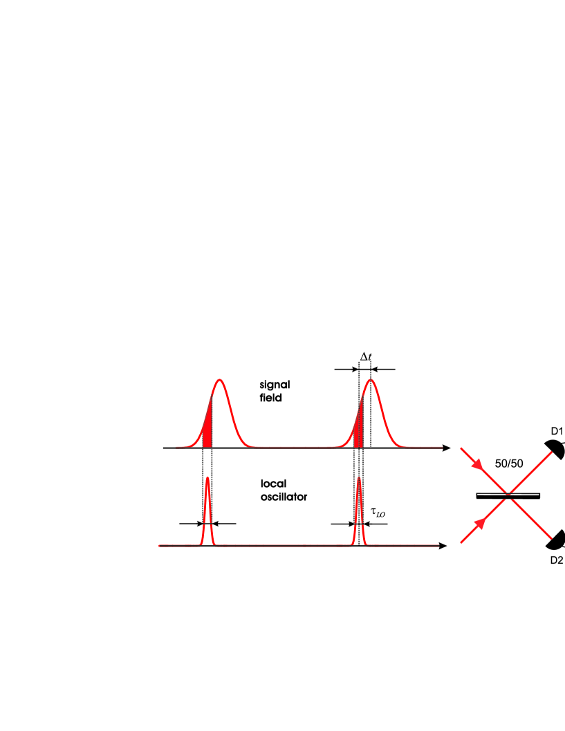
Figure 2: Balanced homodyne detection

Let us now investigate the measurement of field quadratures, obtained by a balanced homodyne detection of the output signal field (see Fig. 2). In this case, the current operator has the well-known form

$$\hat{i}(t)=2\beta(t)\left[\cos\Phi\;\hat{X}_{s}^{out}(t)+\sin\Phi\;\hat{Y}_{s}^{out{\dagger}}(t)\right],$$ (38)

where $\beta(t)e^{i\Phi}$ is the complex amplitude of the local oscillator. Choosing $\Phi=0$ and $\Phi=\pi/2$, one can follow both quadrature amplitudes in the form

$$\hat{i}(t)=2\sum_{n}\beta(t_{n})\left(\begin{array}[]{c}\hat{X}_{s,n}^{out}(t_{n})\\ \\ \hat{Y}_{s,n}^{out}(t_{n})\end{array}\right),\qquad t_{n}=t-nT_{R}$$ (42)

We supposed here that the local oscillator pulses are all identical, that they do not have phase modulation and that their period is equal to the period of signal pulses $T_{R}$. This implies that the envelope does not depend on pulse number $n$. We have made the same assumptions for the SPOPO pumping field. The parameters that can be changed in the homodyne detection setup are the duration of the local oscillator pulses $\tau_{LO}$ as well as their delay $\Delta t$ relative to the signal pulses.

Substituting here the expression (37), we derive the pair correlation functions for the currents in the most general form

$$\left(\begin{array}[]{c}\langle\hat{i}(t)\;\hat{i}(t^{\prime})\rangle_{X}\\ \\ \langle\hat{i}(t)\;\hat{i}(t^{\prime})\rangle_{Y}\end{array}\right)=$$ (46)

$$=\sum_{n}\beta^{2}(t-nT_{R})\left[\delta(t-t^{\prime})\pm\kappa_{s}T_{R}\;\frac{2\mu(t-nT_{R})}{1\mp\mu(t-nT_{R})}e^{\displaystyle-\kappa_{\mp}(t_{n})\;|t-t^{\prime}|}\sum_{n^{\prime}}\delta\left(t-t^{\prime}-nT_{R}+n^{\prime}T_{R}\right)\right].$$ (47)

Here as before we can conclude that in the time domain the quantum effects are of the order $\kappa_{s}T_{R}$ and are therefore very small. We will see in the next section that they appear more clearly on the noise spectra.

A real detector has a finite response time $T_{D}$, and time averages the photodetection signal, so that the observed photocurrent $\hat{I}(t)$ is given by

$$\hat{I}(t)=\frac{1}{T_{D}}\int\limits_{t-T_{D}/2}^{t+T_{D}/2}dt\;\hat{i}(t).$$ (48)

Eq. (47) is valid when $T_{D}$ is much less than $T_{R}$. Let us now consider the case, important in practice, when $T_{R}\ll T_{D}\ll\kappa_{s}^{-1}$. This means that the pulse structure peculiar to the SPOPO is averaged. We expect therefore results looking like the c.w. regime. One gets in this case:

$$\left(\begin{array}[]{c}\langle\hat{I}(t)\;\hat{I}(t^{\prime})\rangle_{X}\\ \\ \langle\hat{I}(t)\;\hat{I}(t^{\prime})\rangle_{Y}\end{array}\right)=\langle I\rangle\;\delta({t-t^{\prime}})\pm\kappa_{s}A_{\mp}(t-t^{\prime}),$$ (52)

where

$$\langle\hat{I}\rangle=\frac{1}{T_{R}}\int\limits_{-T_{R}/2}^{+T_{R}/2}d\tau\;\beta^{2}(\tau),\qquad A_{\mp}(t)=\frac{1}{T_{R}}\int\limits_{-T_{R}/2}^{+T_{R}/2}d\tau\;\beta^{2}(\tau)\frac{2\mu(\tau)}{1\mp\mu(\tau)}e^{\displaystyle-\kappa_{s}\left(1\mp\mu(\tau)\right)|t|}.$$ (53)

By comparison with Eq. (47), wee see that only the equal time feature survives. Let us now choose the pulse of the local oscillator such that $\beta$ as a function of $\tau$ is much narrower than $\mu(\tau)$; then it is possible to use the approximation $\beta^{2}(\tau)=\beta_{0}^{2}\;\delta(\tau)$, so that finally:

$$\left(\begin{array}[]{c}\langle\hat{I}(t)\;\hat{I}(t^{\prime})\rangle_{X}\\ \\ \langle\hat{I}(t)\;\hat{I}(t^{\prime})\rangle_{Y}\end{array}\right)=\langle I\rangle\left[\delta({t-t^{\prime}})\pm\kappa_{s}\frac{2\mu(0)}{1\mp\mu(0)}e^{\displaystyle-\kappa_{s}\left(1\mp\mu(0)\right)|t-t^{\prime}|}\right],\qquad\langle\hat{I}\rangle=\frac{\beta_{0}^{2}}{T_{R}}.$$ (57)

Close to threshold ($1-\mu(0)\ll 1$) we have:

$$\langle\hat{I}(t)\;\hat{I}(t^{\prime})\rangle_{X}/\langle I\rangle=\delta({t-t^{\prime}})+\frac{\kappa_{s}}{1-\mu(0)}\;e^{\displaystyle-\kappa_{s}(1-\mu(0))|t-t^{\prime}|},$$ (58)

$${\langle\hat{I}(t)\;\hat{I}(t^{\prime})\rangle_{Y}}/{\langle I\rangle}=\delta({t-t^{\prime}})-\kappa_{s}\;e^{\displaystyle-2\kappa_{s}|t-t^{\prime}|}.$$ (59)

VI Quantum features on noise spectra

In this section we determine the frequency spectrum of the quantum noise on the $Y$-quadrature. This spectrum is defined as:

$$\left(i^{2}\right)_{\Omega}=\lim_{T\to\infty}\frac{1}{T}\int\limits_{-T/2}^{+T/2}dt\int\limits_{-T/2}^{+T/2}dt^{\prime}\;\langle\hat{i}(t)\;\hat{i}(t^{\prime})\rangle_{Y}\;e^{\displaystyle i\Omega(t-t^{\prime})}.$$ (60)

In the case of $T_{D}\ll T_{R}$, and after substituting Eq. (47) into (60), the spectrum reads:

$$\left(i^{2}\right)_{\Omega}=\frac{1}{T_{R}}\int\limits_{-T_{R}/2}^{+T_{R}/2}dt\;\beta^{2}(t)\left(1-\sum_{m=0,1,2,\cdots}\frac{4\kappa_{s}^{2}\mu(t)}{\kappa_{s}^{2}\left(1+\mu(t)\right)^{2}+\left(\Omega-2\pi m/T_{R}\right)^{2}}\right).$$ (61)

This expression is valid for arbitrary shapes of pump and local oscillator pulses $\mu(t)$ and $\beta(t)$.

In the case of very short local oscillator pulses probing signal ones at their peaks we have the simplified expression:

$${\left(i^{2}\right)_{\Omega}/\langle I\rangle}=1-\sum_{m=0,1,2,\cdots}\frac{4\kappa_{s}^{2}}{4\kappa_{s}^{2}+\left(\Omega-2\pi m/T_{R}\right)^{2}}.$$ (62)

One can see that the quantum noise reduction takes place not only in the vicinity of zero frequency, but also around all resonant frequencies of the cavity $2\pi m/T_{R}$, as known also for the c.w. regime: indeed in the first experiment on generation of squeezed light based on four-wave mixing inside optical cavities Slusher the measured photon pairs were symmetrically shifted with respect to the pump frequency by three cavity mode-spacing frequencies. In Dunlop and Senior squeezing at multiple longitudinal modes of a c.w. degenerate OPO was investigated theoretically and observed experimentally.

The actual frequency response of detectors can be taken into account by multiplying the spectrum (62) by the detector frequency response function Goodman . Obviously a high bandwidth photodetection set-up must be used to observe the noise reduction around multiple resonant frequencies. However if $T_{R}\ll T_{D}\ll\kappa_{s}^{-1}$, then in the spectrum only one quantum feature survives around the zero frequency and its spectrum is given by the well-known formula

$${\left(I^{2}\right)_{\Omega}/\langle I\rangle}=1-\frac{4\kappa_{s}^{2}}{4\kappa_{s}^{2}+\Omega^{2}}.$$ (63)

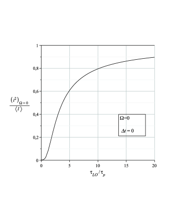
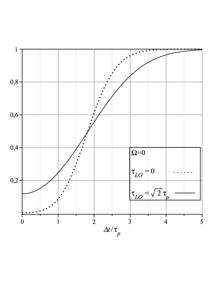
Figure 3: Quantum noise of the squeezed quadrature normalized to the shot noise at zero frequency as a function of duration of local oscillator (LO) pulses (a) and their delay relative to signal ones (b). Both times normalized to pump pulses duration. LO pulses and pump ones are Gaussian. At the Fig. (a) LO pulses are ideally synchronized with signal $\Delta t=0$; at the Fig. (b) two fixed durations of the pulses are considered. In both cases $\kappa_{s}T_{R}=0.1$ and $\mu(0)=0.9$.

Turning back to the general expression (61), one sees that it is nothing else than the time averaged noise spectrum of the signal field quadrature of a c.w. OPO pumped by a c.w. field of instantaneous value $\mu(t)$, weighted by the intensity of the local oscillator pulse. This is a consequence of the fact that different temporal parts of individual pulses of SPOPO are not correlated in our simple model and their nonclassical properties are defined by the instantaneous pump power. Consequently, the detected quantum noise is sensitive to the temporal properties of the local oscillator pulses, particularly to their duration and to the delay relative to signal pulses (see Figures 3 (a) and (b) respectively). As expected the model predicts maximal noise reduction for very short local oscillator pulses ideally synchronized with the signal maxima.

VII Conclusion

In this paper, we have investigated the non-classical properties of a SPOPO operated below threshold using a time-domain approach, in the simplified case when it is possible to neglect the dispersion phenomenon. We have established differential equations for the intracavity field operator amplitude and on this basis investigated the quantum statistical properties of the signal field. As expected the typical region of correlation is the same as for the c.w. regime. However there are supplementary details related to the pulse field structure, namely the fact that different times inside the limits of the same pulse turn out to be uncorrelated, whereas small but nonzero inter-pulse quantum correlations occur between fluctuations at times similarly placed in the different pulses.

We have shown that the ”instantaneous” homodyne signal (i.e. using a local oscillator of very short duration) turns out to be perfectly squeezed when approaching the oscillation threshold from below and at noise frequencies $2\pi m/T_{R}$ ($m=0,1,2,\cdots$), just like in the c.w. case. From a practical point of view the major advantage of the SPOPO is its very low oscillation threshold in terms of mean pump power. This implies that one can use a moderately resonant cavity, with a high escape efficiency, and still have a threshold that can be reached using available mode-locked lasers with average powers in the 100mW range.

Let us mention finally that the Heisenberg-Langevin equations that we have established can be modified straightforwardly to take into account experimental effects such as phase modulation and carrier-envelope phase shift of pump pulses, cavity detuning, and singly resonant operation.

VIII Acknowledgements

We acknowledge helpful discussions with G. Patera. The study was performed within the framework of the Russian-French Cooperation Program ”Lasers and Advanced Optical Information Technologies” and the European Project HIDEAS (grant No. 221906). It was also supported by RFBR (No. 08-02-92504, and No. 08-02-00771). VA acknowledges financial support by French government grant (No. 0185-RUS-B09-0529).

Appendix A Some quantitative estimations

In this appendix we estimate the effects that occur in the propagation of femtosecond pump and signal pulses through a dispersive $\chi^{(2)}$ nonlinear crystal. These processes are the reshaping and chirping of pulses due to group velocity dispersion of the crystal and the pulse temporal walk-off due to mismatch of group velocities. The efficiency of each process can be described by a characteristic propagation distance Becker . The group velocity mismatch of the pump and signal fields ($\upsilon_{p}$ and $\upsilon_{s}$ respectively) is characterized by the propagation distance $L^{GV}$ necessary for a signal pulse to walk through the pump one

$$L^{GV}=\frac{\tau_{p}}{|1/\upsilon_{s}-1/\upsilon_{p}|},$$ (64)

where $\tau_{p}$ is the duration of pump pulses. The linear dispersion of the crystal is characterized by the distance $L^{D}$ over which the initial duration of Gaussian pulse $\tau_{p,s}$ will increase by a factor of $\sqrt{2}$

$$L_{p,s}^{D}=\frac{\tau_{p,s}^{2}}{2\beta_{p,s}}$$ (65)

The efficiency of parametric interaction is characterized by the distance $L^{NL}$

$$L^{NL}=\frac{1}{2\sigma|A_{0}^{peak}|}$$ (66)

where $A_{0}^{peak}$ - pump peak amplitude defined by external pumping as well as duration of pump pulses. For straightforward parametric amplification with a pump peak amplitude the signal wave amplitude grow by a factor of $e$ over this propagation distance.

In Table 1 we present characteristic distances evaluated for the following experimental parameters considered in Patera : pump wavelength $\lambda_{p}=0.4\mu m$, duration of pump pulses - $\tau_{p}=100fs$, c.w. threshold pump power inside the cavity - $P_{th}=25mW$; crystal length - $l=0.1mm$. We have also supposed following duration of signal pulse $\tau_{s}=100fs$ in order to estimate $L_{s}^{D}$ using (65).

crystal	$L^{GV}$, mm	$L_{p}^{D}$, mm	$L_{s}^{D}$, mm ($\tau_{s}=100$ fs)	$L^{NL}$, mm
BBO	$\sim(0.25\div 1)$	$\sim(10\div 20)$	$\sim(20\div 30)$	$\sim 4.7$
KNbO3	$\sim(0.1\div 0.75)$	$\sim(10\div 50)$	$\sim(20\div 40)$	$\sim 1.6$

Table 1: Estimations of characteristic distances

Thus data of the Table 1 show that for used experimental parameters the following relation holds

$$l\leq L^{GV}<L^{NL}<L^{D}$$ (67)

Therefore, in the cases we consider here all the discussed processes can be considered as small perturbations of free propagation of pump and signal fields inside the crystal (both BBO and KNbO₃). More precisely the dispersive reshaping and chirping of envelopes of fields are the weakest processes.

Expression (65) also defines characteristic time for the crystal of given length $l$

$$\tau_{s}^{D}=\sqrt{2\beta_{s}l}$$ (68)

Thus, neglecting crystal dispersion we can correctly describe the field properties only at time scales larger than $\tau_{s}^{D}$. For the present experimental parameters this time is on the order of 6 fs.

Appendix B Derivation of the time-domain equations for the intracavity pulsed field

Let us write the pump and signal fields propagating through the crystal in terms of slowly varying complex envelopes $\hat{A}_{r}(z,t)$ introduced by means of the definition

$$\hat{E}_{r}(z,t)=i\left(\frac{\hbar\omega_{r}}{2n_{r}\varepsilon_{0}cS}\right)^{1/2}e^{-i\omega_{r}t+ik_{r}z}\hat{A}_{r}(z,t),\qquad r=s,p,\qquad(\omega_{p}=2\omega_{s}).$$ (69)

Here $k_{r}=k_{r}(\omega_{r})$ are the pump and signal wave vectors determined by linear dispersion of the crystal; $n_{r}=n_{r}(\omega_{r})$ - the indexes of refraction of the crystal.

Collinear propagation of pump and signal fields inside $\chi^{(2)}$ nonlinear crystal with dispersion is described by following two coupled traveling-wave equations written for operators of complex envelopes of fields Becker

$$\left(\frac{\partial}{\partial z}+\frac{1}{\upsilon_{p}}\frac{\partial}{\partial t}+i\frac{\beta_{p}}{2}\frac{\partial^{2}}{\partial t^{2}}\right)\hat{A}_{p}(z,t)=-\sigma\hat{A}_{s}^{2}(z,t)\;e^{-i\Delta\!kz},$$ (70)

$$\left(\frac{\partial}{\partial z}+\frac{1}{\upsilon_{s}}\frac{\partial}{\partial t}+i\frac{\beta_{s}}{2}\frac{\partial^{2}}{\partial t^{2}}\right)\hat{A}_{s}(z,t)=2\sigma\hat{A}_{p}(z,t)\hat{A}_{s}^{{\dagger}}(z,t)\;e^{i\Delta\!kz}$$ (71)

Here $\sigma$ is the coupling constant, proportional to the nonlinear susceptibility of the crystal $\chi^{(2)}$

$$\sigma=\frac{\chi^{(2)}}{c}\;\sqrt{\frac{\hbar\omega_{p}\;\omega_{s}^{2}}{2\epsilon_{0}cSn_{p}n_{s}^{2}}}.$$ (72)

The inverse group velocities and the dispersions of group velocities are respectively

$$\upsilon_{r}^{-1}=\frac{\displaystyle\partial k_{r}(\omega)}{\displaystyle\partial\omega}|_{\omega=\omega_{r}},\qquad\beta_{r}=\frac{\displaystyle\partial^{2}k_{r}(\omega)}{\displaystyle\partial\omega^{2}}|_{\omega=\omega_{r}}.$$ (73)

Exponents on the right hand sides of equations describe phase mismatch of pump and signal carrying waves along their propagation inside the crystal

$$\Delta\!k=k_{p}(\omega_{p})-2k_{s}(\omega_{s}).$$ (74)

In this paper we consider degenerate regime of SPOPO operation, $\Delta\!k=0$.

These equations assume an instantaneous nonlinear response of the medium and use the approximation of slowly varying envelopes. Also linear dispersion of the crystal is considered up to the second order in the perturbative expansion around the pump and signal carrying frequencies Chirkin . Under these approximations equations do not describe arbitrarily fast dynamics of envelopes of fields, but they are quite reasonable for pulses with duration of tens of femtoseconds.

Let us assume that $\beta_{r}=0$, meaning that the parametric crystal is thin enough so that the dispersive reshaping and chirping of envelopes of fields along their propagation inside the crystal are negligible. Under this approximation second-order time derivatives in equations (70) and (71) are dropped. We also assume the parametric interaction is very weak in a single pass through the nonlinear crystal, so that we can use in the right hand sides of the equations the amplitudes of the free propagating fields. In addition, we will assume for simplicity that the group velocities of the pump and signal fields are equal: $\upsilon_{p}=\upsilon_{s}=\upsilon$. The traveling-wave equations take now the simplified form:

$$\left(\frac{\partial}{\partial z}+\frac{1}{\upsilon}\frac{\partial}{\partial t}\right)\hat{A}_{p}(z,t)=-\sigma\hat{A}_{s}^{2}(0,t-z/\upsilon),$$ (75)

$$\left(\frac{\partial}{\partial z}+\frac{1}{\upsilon}\frac{\partial}{\partial t}\right)\hat{A}_{s}(z,t)=2\sigma\hat{A}_{p}(0,t-z/\upsilon)\hat{A}_{s}^{{\dagger}}(0,t-z/\upsilon)$$ (76)

The solutions of these equations can be easily obtained by replacing the time $t$ by its reduced value $\eta=t-z/\upsilon$ and integrating obtained equations over the crystal length. The solutions read

$$\hat{A}_{p}(l,t)=\hat{A}_{p}(0,t-l/\upsilon)-\sigma l\;{\hat{A}_{s}^{2}(0,t-l/\upsilon)},$$ (77)

$$\hat{A}_{s}(l,t)=\hat{A}_{s}(0,t-l/\upsilon)+2\sigma l\;{\hat{A}_{p}(0,t-l/\upsilon)}\hat{A}_{s}^{{\dagger}}(0,t-l/\upsilon)$$ (78)

Now let this thin parametric crystal be placed inside the high-finesse cavity just near the input mirror (see Fig. 1). Putting the coordinate axis $z$ parallel to the optical axis of the cavity one can couple by the following relation the intracavity field amplitudes $\hat{A}_{r}(L,t)$ and $\hat{A}_{r}(0,t)$ before and after the coupling mirror respectively with the amplitude $\hat{A}^{in}_{r}(0,t)$ of the external field entering the cavity

$$\hat{A}_{r}(0,t)=\sqrt{{\cal R}_{r}}\;\hat{A}_{r}(L,t)+\sqrt{{\cal T}_{r}}\;\hat{A}_{r}^{in}(0,t),$$ (79)

where ${\cal R}_{r}$ and ${\cal T}_{r}$ ($r=p,s$) are reflection and transmission coefficients of the mirror. The slow amplitudes of the input fields defined in the same manner as intracavity ones obey following commutation relations Kolobov_99

$$[\hat{A}_{r}^{in}(z,t),\hat{A}^{in{\dagger}}_{r}(z,t^{\prime})]=\delta(t-t^{\prime}),\quad[\hat{A}_{r}^{in}(z,t),\hat{A}_{r}^{in}(z,t^{\prime})]=0.$$ (80)

Using solutions (77)-(78) obtained under thin crystal approximation and assumption of equal group velocities it is straightforward to write following the relations that couple the amplitudes of fields before and after one round-trip inside the SPOPO cavity

$$\hat{A}_{p}(L,t)=\left(\hat{A}_{p}(0,t-T_{R})-\sigma l\hat{A}_{s}^{2}(0,t-T_{R})\right)\;e^{i\omega_{p}T_{ph,p}},$$ (81)

$$\hat{A}_{s}(L,t)=\left(\hat{A}_{s}(0,t-T_{R})+2\sigma l\hat{A}_{p}(0,t-{T_{R}})\hat{A}_{s}^{{\dagger}}(0,t-T_{R})\right)\;e^{i\omega_{s}T_{ph,s}}$$ (82)

Here $T_{R}$ - round-trip time of pump and signal pulses inside the cavity; $T_{ph,p}$ and $T_{ph,s}$ - round-trip times of pump and signal carrier waves. We assume that the pump and signal carriers are resonant for the cavity so that conditions $\omega_{p}T_{ph,p}=2\pi m$ and $\omega_{s}\;T_{ph,s}=2\pi n$ hold.

Representing continuous slowly varying envelope of the signal field as the following piecewise function:

$$\hat{A}_{s}(0,t)=\sum_{n}\hat{A}_{s,n}(t-nT_{R})$$ (83)

and combining (79) with (82) one obtains

$$\hat{A}_{s,n}(t-nT_{R})=\sqrt{{\cal R}_{s}}\left(\hat{A}_{s,n-1}(t-(n-1)T_{R})+2\sigma l\;{\hat{A}_{p,n-1}(t-(n-1)T_{R})}\hat{A}_{s,n-1}^{{\dagger}}(t-(n-1)T_{R})\right)+$$

$$+\sqrt{{\cal T}_{s}}\;\hat{A}_{s,n}^{in}(t-nT_{R}),$$ (84)

where the time $t$ is treated as the time deviation from the pulse center. We see that there are actually two time arguments, because the index $n$ informs us about exchanges from pulse to pulse. Strictly speaking this second argument is discrete with distance between adjoining point equal to $T_{R}$. However assuming that the pulse envelope does not change essentially after one round trip inside the cavity one can neglect the time interval $T_{R}$ in comparison with other typical. This enables us to consider the time variable $T$ as continuous. Such a two-time approach has been used in Ref. Haus for description of pulsed lasers. We can then make the following replacements in Eq. (84)

$$\hat{A}_{r,n}(t-nT_{R})\to\hat{A}_{r}(t,T)\;(r=p,s),\qquad\frac{\hat{A}_{s,n}(t-nT_{R})-\hat{A}_{s,n-1}(t-(n-1)T_{R})}{T_{R}}\to\frac{\partial\hat{A}_{s}(t,T)}{\partial T}$$ (85)

We can finally use the same procedure to get the equation for the pump pulse amplitude. We have then justified in this appendix the introduction of equations  (6) and (7) of the present paper.

Figure 1: Synchronously pumped OPO

References

- (1) H.-A. Bachor, T.C. Ralph, A Guide To Experiments In Quantum Optics, 2nd ed. (Wiley-VCH, Berlin, 2003).
- (2) R.E. Slusher, L.W. Hollberg, B. Yurke, J.C. Mertz, J.F. Valley, Phys. Rev. Lett. 55, 2409 (1985).
- (3) G.J. de Valcárcel, G. Patera, N. Treps, C. Fabre, Phys. Rev. A 74, 061801 (2006).
- (4) N.C. Menicucci, S.T. Flammia, O.Pfister, Phys. Rev. Lett. 101, 130501 (2008).
- (5) Lectures on Quantum Information, edited by D. Bru, G. Leuchs (Wiley-VCH, Berlin, 2003).
- (6) B. Lamine, C. Fabre, and N. Treps, Phys. Rev. Lett. 101, 123601 (2008).
- (7) G. Patera, N.Treps, C. Fabre, G.J. de Valcárcel, Eur. Phys. J. D 56, 123 (2010).
- (8) F. Rana, R.J. Ram, H. Haus, IEEE Journal of Quantum Electronics 40, 41 (2004).
- (9) M.I. Kolobov, Rev. Mod. Phys. 71, 1539 (1999).
- (10) S. Reynaud, C.Fabre, E.Giacobino, J. Opt. Soc. Am. B 4, 1520 (1987).
- (11) A.E. Dunlop, E.H. Huntington, C.C. Harb, T.C. Ralph, Phys. Rev. A 73, 013817 (2006).
- (12) R.J. Senior et al, Optics Express 15, 5310 (2007).
- (13) J.W. Goodman, Statistical Optics (Wiley-Interscience, New York, 1985).
- (14) M.F. Becker, D.J. Kuizenga, D.W. Phillion, A.E. Siegman, Journal of Applied Physics 45, 3996 (1974).
- (15) S.A. Akhmanov, V.A. Vysloukh, A.S. Chirkin, Optics of Femtosecond Laser Pulses (1992).