A slip model for micro/nano gas flows induced by body forces

Abstract

A slip model for gas flows in micro/nano channels induced by external body forces is derived based on Maxwell’s collision theory between gas molecules and the wall. The model modifies the relationship between slip velocity and velocity gradient at the walls by introducing a new parameter in addition to the classic Tangential Momentum Accommodation Coefficient. Three-dimensional Molecular Dynamics simulations of helium gas flows under uniform body force field between copper flat walls with different channel height are used to valid the model and to determine this new parameter.

NOMENCLATURE

$\lambda$	Mean free path
$H,B,L$	Channel height, width and length
Kn	Knudsen number
$n,\rho$	Number density, mass density
$d$	Molecular diameter
$L_{s},L^{*}_{s}$	Slip length, dimensionless slip length
$x,y,z$	Cartesian coordinate
$\hat{z}$	Normalized coordinate
$\sigma_{v}$	Tangential Momentum Accommodation Coefficient
$v,\hat{v}$	Tangential velocity, normalized tangential velocity
$v_{slip},\hat{v}_{slip}$	Slip velocity, normalized slip velocity
$v_{ref}$	Reference velocity
$N^{\pm}$	Molecules going upward $N^{+}$ and downward $N^{-}$
	with respect to the control surface $s$
$N$	Total number of molecules passing through $s$
$<v^{\pm}_{x}>$	Average velocity of molecules going upward $<v_{x}^{+}>$
	and downward $<v_{x}^{-}>$ with respect to $s$
$v_{s},v_{w}$	Gas velocity near the wall, velocity of the wall
$<\tau>,\bar{c}$	Mean collision time, thermal speed
$k_{B},T$	Boltzmann constant, absolute temperature
$m,\gamma_{x}$	Molecular mass, acceleration along x-axis
$\alpha,\beta$	Slip parameters of the present model
$v_{\lambda}$	Gas velocity at distance $\lambda$ from the wall
$\mu,\mu^{*},\bar{\mu}$	Gas viscosity, scaled viscosity, kinetic theoretical
	viscosity
$V_{i}$	Potential energy of atom $i$
$F,\rho_{e},\phi$	Potential functions of Embedded Atom Model
$\sigma_{a-b},\epsilon_{a-b}$	Parameters of Lennard Jones potential between
	molecules $a$ and $b$
$r_{ij}$	Distance between two molecules $i$ and $j$.

1 Introduction

The velocity of a fluid close to a solid wall is always different from the wall velocity even if the latter is perfectly diffusive. Especially, when the channel height is decreased to that of MEMS or NEMS devices (Micro/Nano Electro-Mechanical Systems), this phenomenon becomes highly important and must be taken into account. The Knudsen number $\mathrm{Kn}$, the ratio between the mean free path $\lambda$ and the characteristic length of the channel $H$, is the relevant parameter to quantify the slip effects. The mean free path $\lambda$ is usually defined as the average distance that molecules travel between collisions and equal to

$$\lambda=\frac{1}{{\sqrt{2}n\pi d^{2}}}$$ (1)

where $n$ is number density and $d$ is the effective molecular diameter. According to Maxwell’s model maxwell1879srg , the slip length $L_{s}$ in continuous fluid mechanics can be determined via the Tangential Momentum Accommodation Coefficient, also denoted by TMAC or $\sigma_{v}$ as follows

$$L_{s}=\frac{2-\sigma_{v}}{\sigma_{v}}\lambda$$ (2)

The slip velocity, $v_{slip}$ is calculated by the formula

$$v_{slip}=L_{s}\left.\frac{\partial v}{\partial z}\right|_{w}$$ (3)

The term $\left.\frac{\partial v}{\partial z}\right|_{w}$ is the normal derivatives of the tangential velocity component at the walls, assuming that the normal to the wall is in the z-direction. If the velocity and coordinate in Eq. (3) are scaled with a reference velocity $v_{ref}$ and the channel height H, we have

$$\hat{v}_{slip}=L^{*}_{s}\left.\frac{\partial\hat{v}}{\partial\hat{z}}\right|_{w},\quad L^{*}_{s}=\frac{L_{s}}{H}$$ (4)

where $\hat{v}_{slip}=v_{slip}/v_{ref}$ and $\hat{z}=z/H$. The term $L^{*}_{s}$ is called the dimensionless slip length and equal to

$$L^{*}_{s}=\frac{2-\sigma_{v}}{\sigma_{v}}\mathrm{Kn}$$ (5)

when the Maxwell model is used. Consequently, for a given accommodation coefficient, Eq. (5) predicts that $L^{*}_{s}$ is proportional to Kn. When Kn tends towards zero, we recover the no slip condition and when Kn increases, the slip effect increases. The Maxwell model is widely used to describe the slip at the walls because it only needs one parameter only, $\sigma_{v}$.

The physical meaning of $\sigma_{v}$ in (2,5) is that if $M$ molecules arrive at the wall, $\sigma_{v}M$ of them are reflected diffusively and the remaining $(1-\sigma_{v})M$ molecules are reflected specularly. Based on Eq. (2), one can determine TMAC by either experiments or Molecular Dynamics (MD) simulations. Some experimentalists controlled macroscopic quantities such as pressure and mass flow rate and made use of the relationship with the slip velocity to find TMAC (see e.g. arkilic2001mfa ; colin2004vso ). Arkilic et al. arkilic2001mfa studied flows of nitrogen, argon and carbon dioxide through rectangular silicon channels and found TMAC ranging between 0.75 and 0.85. Colins et al. colin2004vso worked on the couples silicon-nitrogen and silicon-helium and found a relatively high coefficient, 0.93. Recently, Maali and Bhushan maali2008slm studied confined air flow between a spherical glass particle glued to the cantilever of an atomic force microscopy (AFM) and a glass plate. They let the cantilever oscillating and measured the hydrodynamic damping factor. Consequently, a value of the slip length of about 118 nm was obtained. It corresponds to an accommodation coefficient of 0.72. Direct measurements of TMAC on the couple He-Cu by Seidl (see finger2007mds ; gadelhak1999fmm ) stated that the coefficient depends on the collision angle between gas and solid, ranging from 0.6 to 1.0. On the other hand, Cao et al. cao2004agm ; cao2005tdt ; cao2006esr using MD approaches to simulate flows, revealed that TMAC at Ar-Pt interface can be as small as 0.2 and influenced by temperature and surface roughness. Arya et al. Arya2003msk simulated directly the collisions between gas and wall. Their results showed the dependence of TMAC on the wall’s lattice structure. It remains constant as long as the drift velocity is small enough (less than 100 m/s). Finger et al. finger2007mds used similar method as Arya2003msk to show that TMAC is affected by the adsorbed layer and their results matched the previous experiment of Seidl on the couple copper-helium. Generally speaking, both experimental and MD works gave a rather scattering results of TMAC and reflected the dependency of TMAC on many factors. Hence, this coefficient should be understood as an effective one and to be used with caution.

Extensions of Maxwell’s model to different configurations have been considered in the past. When the Knudsen number increases, Beskok (see karniadakis2005man ; gadelhak1999fmm and the references cited therein) argued that higher order of the Knudsen number and higher order derivatives of velocity must be used in the slip equations. For curved surface, Lockerby et al. lockerby2004vbc accounted for the contribution of normal velocity in the viscous stress. In all the aforementioned works, the gas molecules are not subject to any external forces before arriving at the wall, which is not applicable in the presence of volume force field such as gravity, electrostatics, etc… With these force fields, the slip velocity is different from flows driven by pressure gradient and cannot be simply described by (2). In what follows, on the basis of kinetic theory, we derive the new slip equation that accounts for the external body force field.

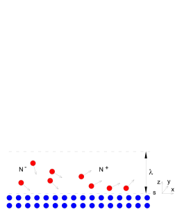
Figure 1: Collision model between gas molecules and a solid wall. $N^{-}$ and $N^{+}$ are respectively the number of molecules going downward and upward and passing through the surface $s$ near the wall within one unit time. If there is no accumulation of gas near the wall, $N^{-}=N^{+}$.

2 Slip model for micro/nano gas flows induced by body force

In the following derivation, the gas flow is assumed to be isothermal so that the influence of temperature on the slip velocity is not taken into account. Using the similar approach of Beskok (see karniadakis2005man ), let us consider a control surface $s$ near and parallel to the wall (see Fig. 1). For a unit time, there are $N$ gas molecules passing through the surface which are composed of $N^{-}$ molecules going downward and $N^{+}$ going upward with respectively average tangential velocities, $<v_{x}^{-}>$ and $<v_{x}^{+}>$. The gas average tangential velocity at the wall $v_{s}$ may be written as

$$N^{+}<v_{x}^{+}>+N^{-}<v_{x}^{-}>=Nv_{s}$$ (6)

The molecules that go upward are those that previously went downward and were reflected at the surface $s$. Because the reflection is either diffusive or specular by the fractions $\sigma_{v}$ and $1-\sigma_{v}$, the following relation holds for a wall moving at velocity $v_{w}$:

$$N^{+}<v_{x}^{+}>=(1-\sigma_{v})N^{-}<v_{x}^{-}>+\sigma_{v}N^{-}v_{w}$$ (7)

which is equivalent to

$$Nv_{s}=N^{-}\left[<v_{x}^{-}>+(1-\sigma_{v})<v_{x}^{-}>+\sigma_{v}v_{w}\right]$$ (8)

Without external volume force, the $N^{-}$ molecules colliding with the wall come from one mean free path $\lambda$ away from the wall without collision so that their velocity does not change $<v_{x}^{-}>=v_{\lambda}$. We also assume that $N^{-}=N^{+}=N/2$. It follows

$$2v_{s}=\left[(2-\sigma_{v})v_{\lambda}+\sigma_{v}v_{w}\right]$$ (9)

The Taylor development of $v_{\lambda}$ near the wall, $v_{\lambda}=v_{s}+\lambda\left.\frac{\partial v}{\partial z}\right|_{w}$, gives the relation for slip velocity $v_{slip}$ defined as $v_{s}-v_{w}$ (first order Maxwell’s relationship)

$$v_{slip}=\alpha\left.\lambda\frac{\partial v}{\partial z}\right|_{w}\quad\mathrm{with}\quad\alpha=\frac{2-\sigma_{v}}{\sigma_{v}}$$ (10)

In the presence of uniform volume force, i.e. in the case where a constant acceleration $\gamma_{x}$ is applied on each gas molecule, $<v_{x}^{-}>$ is no longer equal to $v_{\lambda}$. When impinging at the wall surface, the term $\gamma_{x}\beta<\tau>$ should be added to the average tangential velocity

$$<v_{x}^{-}>=v_{\lambda}+\gamma_{x}\beta<\tau>.$$ (11)

Above, $<\tau>$ is the mean time for the molecules to arrive at the surface after the previous collision and is assumed to be $\lambda/\bar{c}$ where $\bar{c}$ is the thermal speed of the gas. For gases in local equilibrium, the thermal speed is estimated by $\bar{c}=\sqrt{2k_{B}T/m}$. The constant $\beta$, introduced in the last term of (11), can be seen as a factor which accounts for the differences between the idealized conditions used to derive the slip model and the realistic ones. In reality, these differences can be due to the following reasons
- the wall in the model is idealized as a surface and the gas wall collisions only take place at this surface. In fact, the wall also has an atomistic structure and the interaction force must be taken into account at distance of several molecular diameters.
- after arriving at the wall, the gas molecules can stay near the wall during a finite duration of time before leaving.

The value of $\beta$ is expected to be close to unity. The slip equation with the corrected term becomes

$$v_{slip}=\alpha\lambda\left[\beta\frac{\gamma_{x}}{\bar{c}}+\left.\frac{\partial v}{\partial z}\right|_{w}\right]$$ (12)

Equation (12) is the new slip equation for general flows in which the body force is involved. In what follows, we study a particular case where the gas flow of viscosity $\mu$ is induced by a constant body force $\rho\gamma_{x}$ along one direction $x$. Without pressure gradient, the velocity profile is given by

$$v(z)=\frac{\rho\gamma_{x}}{2\mu}\left(\frac{H^{2}}{4}-z^{2}\right)+v_{slip},$$ (13)

which after combined with the new slip model equation (12) yields the dimensionless form

$$\frac{\bar{c}\,v_{slip}}{\lambda\gamma_{x}}=\alpha\left[\beta+\frac{1}{\mu^{*}\mathrm{Kn}}\right],\quad\mu^{*}=\frac{\mu}{\bar{\mu}}.$$ (14)

In the above equation, $\mu^{*}$ is the scaled viscosity and $\bar{\mu}$ is the kinetic theoretical viscosity liou03mm ; struchtrup2005mte defined as $\bar{\mu}=\frac{1}{2}\rho\lambda\bar{c}$. The dimensionless slip length $L_{s}^{*}$ can be calculated accordingly

$$L_{s}^{*}=\alpha\mathrm{Kn}\left[\beta\mu^{*}\mathrm{Kn}+1\right]\quad\mathrm{with}\quad L_{s}^{*}=L_{s}/H$$ (15)

We can deduce that the derived slip length is second-order dependent of the Knudsen number. The influence of the volume force on the slip length becomes thus important when $\mathrm{Kn}$ is large enough. The ratio $L_{s}^{*}/\mathrm{Kn}$ is no longer equal to the constant $\alpha$ but is dependent on the channel characteristic dimension $H$ via a composite parameter $(\mu^{*}\mathrm{Kn})^{-1}$. If $\mathrm{Kn}$ is increased and the variation of fluid viscosity $\mu$ is small, we shall observe an increase in the ratio $L_{s}^{*}/\mathrm{Kn}$. In what follows, we use the molecular dynamics approach to valid this prediction and determine as well the two new model parameters $\alpha$ and $\beta$.

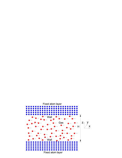
Figure 2: One dimensional flow induced by external volume force. The simulation domain is periodic in directions $x,y$. The external volume force in direction $x$ is produced by applying additional constant acceleration $\gamma_{x}$ on each gas atoms.

3 Molecular dynamics validation

In order to recover the dependence of slip velocities on the Knudsen number and volume force, we simulate a flow induced by uniform external volume force. The gas/solid couple investigated is helium (He) and copper (Cu). The choice of the couple He-Cu is motivated by two reasons: firstly, the accommodation coefficients derived experimentally and numerically are shown to be in good agreement (see for example ref. finger2007mds ) and, secondly the interaction potentials between these atomic species have been widely used (see ref. foiles86eam ; daw1984eam ; plimpton1995fpa ; finger2007mds ; allen1989csl ). However, the present method can be applied to any gas/wall system as long as the interaction potential between the atoms is properly provided. Because the slip length depends on what happens at the interface, the final results are strongly affected by the choice of the system.

The channel is made of two parallel solid walls, each of them contains 9 layers (or 4 lattice units) of Cu atoms placed at fcc lattice sites. The lattice constant is chosen initially equal to 3.615 Å. The interaction forces between Cu atoms are derived from the EAM potential foiles86eam ; daw1984eam

$$V_{i}=F\left[\sum_{j}\rho_{e}(r_{ij})\right]+\frac{1}{2}\sum_{i\neq j}\phi(r_{ij})$$ (16)

where $V_{i}$ is the potential energy of atom $i$ composed of the binary potential $\phi(r_{ij})$ and embedded potential $F$ accounting for electron density contribution $\rho_{e}$. The interaction forces for the couples He-He and He-Cu are derived from the widely used Lennard-Jones potential

$$V_{i}=\sum_{j}4\varepsilon\left[\left({\frac{\sigma}{r_{ij}}}\right)^{12}-\left(\frac{\sigma}{r_{ij}}\right)^{6}\right]$$ (17)

The parameters used in this paper are those from allen1989csl ; finger2007mds , $\varepsilon_{He-He}=0.00088$ eV, $\sigma_{He-He}=2.28$ Å, $\varepsilon_{He-Cu}=0.0225$ eV, $\sigma_{He-Cu}=2.29$ Å. The He-Cu parameters have been calculated using the Lorentz-Berthelot mixing laws from the He-He and Cu-Cu parameters in allen1989csl . The last atom layer at the two walls is fixed (see Fig. 2). The remaining atoms of the wall and the gas are maintained at the same temperature $120$ K by a usual scaling method after removal of the mean velocity. On average, the wall is kept immobile, i.e $v_{w}=0$.

In this work, the global number density of the gas are kept constant $n=0.0026$ Å^-3 (or $\rho=1.78\times 10^{-14}$ pg/ų) while the channel height $H$ and acceleration $\gamma_{x}$ is varied to obtain results for different global Knudsen numbers and volume forces $f$. At the small density number and temperature of our simulations (e.g. 120 K), the helium is in gaseous phase. Three values of $H=361$, 260 and 174 Å  corresponding respectively to Kn=0.046, 0.064, 0.098 are considered. These three Kn numbers are chosen to fall into the range $(0.01,0.1)$ in order to assure the slip flow regimes in our test cases according to karniadakis2005man . The two other dimensions of the simulation box along x-axis (the flow direction) and along y-axis denoted shortly by length $L$ and width $B$ are $L=H$ and $B=H/2$. For each channel height, the acceleration applied on each atom is varied as $\gamma_{x}=0.0036$, 0.012, 0.024 Å/ps². The computations are carried out by using LAMMPS, an open source parallelized code plimpton1995fpa on an IBM Power6 machine. The equations of the particle motion are integrated using a Leapfrog-Verlet algorithm with a time step $0.002$ ps. The steady state is achieved after $5\times 10^{6}$ time steps and it takes another $2\times 10^{6}$ time steps for the average process. All the models are constructed in 3D with the parameters given in Table 1. Due to the high density of the solid wall, an important number of Cu atoms are considered. The largest model, case Kn=0.046, involves 289 500 molecules and takes 8 hours of computation on 512 processors.

Table 1: Size of the simulation box and number of helium and copper atoms for different Knudsen numbers

Kn	H [Å]	L [Å]	B [Å]	Cu atoms	He atoms
0.046	361	361	180	230 700	58 800
0.064	260	260	130	51 840	22 680
0.098	174	174	87	23 040	6 624

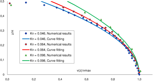
Figure 3: Velocity profiles for the upper half of the channel obtained by MD simulation (marker line) and fitted by analytical formula (solid line). In the figure, the acceleration $\gamma_{x}$ is kept constant at $0.012$ Å/ps² while the Knudsen number is varied. The vertical and horizontal axis represent normalized coordinate $z/H$ and velocity $v(z)/v_{\max}$ along the flow direction. The velocity $v_{\max}$ is the maximal velocity found in the middle of the channel.

In order to obtain accurate solutions, the channel has been divided in a sufficiently large number of layers for the average procedure. For $\gamma_{x}=0.012$ Å/ps² and different Knudsen numbers, the velocity profiles in the upper half channel are plotted in Fig. 3. We find good agreement between analytical solution (Eq. 13) and the numerical results in the major part of the channel. The global viscosity of the fluid $\mu$ and slip velocity $v_{slip}$ are obtained by fitting the numerical velocity profiles (Fig. 3) with equation (13), given in columns 3, 4 of Table 2. It is noted that the determination of $\mu$ is based the curvature of the velocity profile and the average density $\rho$, regardless of the redistribution of density at the steady state.

Table 2: Numerical results from MD simulations

Kn	$\gamma_{x}$	$\mu\times 10^{5}$	$v_{slip}$	$\frac{L_{s}^{*}}{\mathrm{Kn}}$	$\frac{1}{\mu^{*}\mathrm{Kn}}$	$\frac{\bar{c}\,v_{slip}}{\lambda\gamma_{x}}$
	[Å/ps2]	[Pa.s]	[Å/ps]
0.046	0.0036	1.89	0.18	1.87	11.60	21.80
	0.012	1.91	0.54	1.69	11.50	19.40
	0.024	2.00	1.38	2.20	11.30	25.00
0.064	0.0036	1.95	0.14	1.97	8.05	15.80
	0.012	2.02	0.43	1.91	7.77	14.90
	0.024	2.11	0.89	2.10	7.44	15.50
0.098	0.0036	2.03	0.08	1.90	5.08	9.41
	0.012	2.31	0.27	2.12	4.48	9.51
	0.024	2.27	1.38	2.26	4.54	10.03

From the results reported in Table 2, it can be seen that $L_{s}^{*}/\mathrm{Kn}$ tends to increase with $\mathrm{Kn}$. This trend cannot be accounted for by the usual one parameter model. In order to determine the two constants $\alpha$ and $\beta$ in our proposed model (see Eq. 14), we plotted two dimensionless quantities $\frac{\bar{c}\,v_{slip}}{\lambda\gamma_{x}}$ and $(\mathrm{Kn}\mu^{*})^{-1}$ from the last two columns of Table 2 into Fig. 4. We found the straight line that best fits these data. In the framework of our problem, the two values $\alpha=1.81$ and $\beta=0.76$ were determined. As expected, the value $\beta$ is of order unity while $\alpha$ corresponds to an accommodation coefficient $\sigma_{v}=0.71$ which is in the experimental range [$0.66$, $1.0$] by Seidl, reported in the paper of finger2007mds for the couple He-Cu. It is noted that these two bound limits $0.66$ and $1.0$ correspond to the two extreme impinging at angles $70\textdegree$ and $10\textdegree$ of helium molecules at a copper wall in Seidl’s experiments (see Tab. 3).

Table 3: Seidl experimental data on the couple He-Cu (see finger2007mds ) where TMAC depends on the collision angle of the gas molecules

Angle	Seidl	Seidl lower	Seidl upper
	variability	TMAC value	TMAC value
10	0.100	0.86	1.06
20	0.080	0.81	0.97
30	0.065	0.77	0.90
40	0.050	0.73	0.83
50	0.040	0.71	0.79
60	0.030	0.69	0.75
70	0.020	0.66	0.70

The impact of parameter $\beta$ on slip velocity depends on the relative importance between the two terms $\beta$ and $(\mathrm{Kn}\mu^{*})^{-1}$. For large Kn, the role of coefficient $\beta$ becomes important, e.g. up to $20\%$ when Kn = 0.098 while for small Kn, e.g. Kn = 0.046, this effect is almost negligible ($6\%$). In order to compare with the classical model that involves a single parameter $\alpha$, the numerical results are also fitted with a line passing through origin, the dashed line in Fig. 4. The coefficient $\alpha$ predicted by the classical model takes the higher value $\alpha=1.95$ and shows more discrepancies with respect to the simulation results.

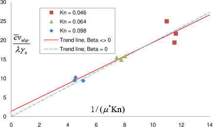
Figure 4: Relations between two dimensionless quantities $\frac{\bar{c}\,v_{slip}}{\lambda\gamma_{x}}$ and $1/(\mathrm{Kn}\mu^{*})$. The solid line represents the equation (14) which fits the numerical results. This line makes an angle $\arctan\alpha$ with the horizontal axis and cuts the vertical axis at $\alpha\beta$. The dashed line represents (14) with $\beta=0$ that fits the numerical results.

4 Concluding remarks and discussion

A new slip model for flows with volume force has been introduced. Two parameters with physical meanings that relates slip velocity and velocity gradient at walls are suggested. The first one is the traditional tangential momentum accommodation coefficient, as in the widely used Maxwell model, while the second one accounts for the additional velocity that a molecule encompasses owing to the applied force before striking at a the solid surface. Molecular dynamics calculations applied on the He-Cu couple allowed to determine both TMAC and the new parameter $\beta$ introduced in the present work. TMAC is found to be in good agreement with experimental data. In the $v_{slip}$ expression, the effect of parameter $\beta$ increases with $\mathrm{Kn}$, i.e. when the limit of transitional flow is reached.

The present model is useful for the global analysis of flows without knowing the presence of the Knudsen layer. In our MD simulations, both higher density and slower motion of gas molecules are observed near the walls and cause deviation of the numerical velocity from the Navier-Stokes solution. Similar phenomenon was encountered and discussed in cao2005tdt from molecular viewpoint. Generally, when a molecule reaches a surface, it does not bounce back immediately but is often trapped by the potential well. The molecules remains near the wall for some time, interacts with many other solid atoms before escaping. Accounting for the Knudsen layer should leads to more accurate results (see Lockerby et al. lockerby2005uhoc ; lockerby2008modelling ). A model involving body force as well as Knudsen layer may be expected in the near future.

- (1) Maxwell J, On stresses in rarified gases arising from inequalities of temperature, Philos T Roy Soc A, 170, 231-256 (1879).
- (2) Arkilic, E., Breuer, K., Schmidt, M, Mass flow and tangential momentum accommodation in silicon micromachined channels, J Fluid Mech, 437, 29-43 (2001).
- (3) Colin, S., Lalonde, P., Caen, R, Validation of a second-order slip flow model in rectangular microchannels, Heat Transfer Eng, 25, 23-30 (2004).
- (4) Maali, A., Bhushan, B., Slip-length measurement of confined air flow using dynamic atomic force microscopy, Phys Rev E, 78, 027302 (2008).
- (5) Finger, G., Kapat, J., Bhattacharya, A., Molecular dynamics simulation of adsorbent layer effect on tangential momentum accommodation coefficient, J Fluid Eng-T Asme, 129, 31-39 (2007).
- (6) Gad-el-Hak, M, The fluid mechanics of microdevices-the freeman scholar lecture, J Fluid Eng-T Asme, 121, 5-33 (1999).
- (7) Cao, B., Min, C., Guo, Z, Application of 2DMD to gaseous microflows, Chinese Sci Bull, 49, 1101-1105 (2004).
- (8) Cao, B., Chen, M., Guo, Z, Temperature dependence of the tangential momentum accommodation coefficient for gases, Appl Phys Lett, 86, 091905 (2005).
- (9) Cao, B., Chen, M., Guo, Z, Effect of surface roughness on gas flow in microchannels by molecular dynamics simulation, Int J Eng Sci, 44, 927-937 (2006).
- (10) Arya, G., Chang, H.-C., Maginn, E. J, Molecular simulations of Knudsen wall-slip: effect of wall morphology, Mol Simulat, 29, 697-709, (2003).
- (11) Karniadakis, G., Beskok, A., Aluru, N., Microflows and nanoflows: Fundamentals and simulation, Springer, New York (2005).
- (12) Lockerby, D. A., Reese, J. M., Emerson, D. R., Barber, R. W., Velocity boundary condition at solid walls in rarefied gas calculations, Phys Rev E, 70, 017303 (2004).
- (13) Liou, W., Fang, Y., Microfluid Mechanics, McGraw-Hill, New York (2003).
- (14) Struchtrup, H., Macroscopic Transport Equations for Rarefied Gas Flows: Approximation Methods in Kinetic Theory, Springer, New York (2005).
- (15) Foiles, S. M., Baskes, M. I., Daw, M. S, Embedded-atom-method functions for the fcc metals Cu, Ag, Au, Ni, Pd, Pt, and their alloys, Phys Rev B, 33, 7983-7991 (1986).
- (16) Daw, M. S., Baskes, M. I., Embedded-atom method: Derivation and application to impurities, surfaces, and other defects in metals, Phys Rev B, 29, 6443-6453 (1984).
- (17) Plimpton, S., Fast parallel algorithms for short-range molecular dynamics, J Comput Phys, 117, 1-19 (1995).
- (18) Allen, M., Tildesley, D., Computer Simulation of Liquids, Oxford University Press, Oxford (1989).
- (19) Lockerby, D. A., Reese, J. M., Gallis, M. A, The usefulness of higher-order constitutive relations for describing the Knudsen layer, Phys Fluids, 17, 100609 (2005).
- (20) Lockerby, D. A., Reese, J. M., On the modelling of isothermal gas flows at the microscale, J Fluid Mech, 604, 235-261 (2008).