A consistent test of independence based on a sign covariance related to Kendall’s tau

Abstract

The most popular ways to test for independence of two ordinal random variables are by means of Kendall’s tau and Spearman’s rho. However, such tests are not consistent, only having power for alternatives with “monotonic” association. In this paper, we introduce a natural extension of Kendall’s tau, called $\tau^{*}$, which is non-negative and zero if and only if independence holds, thus leading to a consistent independence test. Furthermore, normalization gives a rank correlation which can be used as a measure of dependence, taking values between zero and one. A comparison with alternative measures of dependence for ordinal random variables is given, and it is shown that, in a well-defined sense, $\tau^{*}$ is the simplest, similarly to Kendall’s tau being the simplest of ordinal measures of monotone association. Simulation studies show our test compares well with the alternatives in terms of average $p$-values.

and

1 Introduction

A random variable $X$ is called ordinal if its possible values have an ordering, but no distance is assigned to pairs of outcomes. Ordinal variables may be continuous, categorical, or mixed continuous/categorical. Ordinal data frequently arise in many fields, though especially often in social and biomedical science (Kendall and Gibbons [13], Agresti [1]). Ordinal data methods are also often applied to real-valued (interval level) data in order to achieve robustness.

(a) Concordant pair	(b) Discordant pair

Figure 1: Concordant and discordant pairs of points associated with Kendall’s tau.

(a) Concordant triples			(b) Discordant triples

Figure 2: Concordant and discordant triples of points associated with Spearman’s rho.

The two most popular measures of association for ordinal random variables $X$ and $Y$ are Kendall’s tau ($\tau$) (Kendall [14]) and Spearman’s rho ($\rho_{S}$) (Spearman [25]), which may be defined as

$$\tau=E\operatorname{sign}\bigl{[}(X_{1}-X_{2})(Y_{1}-Y_{2})\bigr{]},\qquad\rho_{S}=3E\operatorname{sign}\bigl{[}(X_{1}-X_{2})(Y_{1}-Y_{3})\bigr{]},$$

where the $(X_{i},Y_{i})$ are independent replications of $(X,Y)$ (Kruskal [16]). The factor 3 in the expression for $\rho_{S}$ occurs to obtain a measure whose range is $[-1,1]$. Both $\tau$ and $\rho_{S}$ are proportional to sign versions of the ordinary covariance, which can be seen from the following expressions for the covariance:

$$\operatorname{cov}(X,Y)={\textstyle\frac{1}{2}}E(X_{1}-X_{2})(Y_{1}-Y_{2})=E(X_{1}-X_{2})(Y_{1}-Y_{3}).$$

From the definitions, probabilistic interpretations of $\tau$ and $\rho_{S}$ can be derived. Firstly,

$$\tau=\Pi_{C_{2}}-\Pi_{D_{2}},$$ (1)

where $\Pi_{C_{2}}$ is the probability that two observations are concordant and $\Pi_{D_{2}}$ the probability that they are discordant (see Figure 1). Secondly,

$$\rho_{S}=\Pi_{C_{3}}-\Pi_{D_{3}},$$

where $\Pi_{C_{3}}$ is the probability that three observations are concordant and $\Pi_{D_{3}}$ the probability that they are discordant (see Figure 2). It can be seen that $\tau$ is simpler than $\rho_{S}$, in the sense that it can be defined using only two rather than three independent replications of $(X,Y)$, or, more specifically, in terms of probabilities of concordance and discordance of two rather than three points. This was a reason for Kruskal to prefer $\tau$ to $\rho_{S}$ (Kruskal [16], end of Section 14).

An alternative definition of $\rho_{S}$, which was originally given by Spearman, is as a Pearson correlation between uniform rank scores of the $X$ and $Y$ variables. For continuous random variables, both this and the aforementioned definition lead to the same quantity. However, with this definition, $\rho_{S}$ is to some extent an ad hoc measure, since the choice of scores is arbitrary, and alternative scores (e.g., normal scores) might be used.

A test of independence based on i.i.d. data can be obtained by application of the permutation test to an estimator of $\tau$ or $\rho_{S}$, which is easy to implement and fast to carry out with modern computers. Such ordinal tests are also used as a robust alternative to tests based on the Pearson correlation.

A drawback for certain applications is that $\tau$ and $\rho_{S}$ may be zero even if there is an association between $X$ and $Y$, so tests based on them are inconsistent for the alternative of a general association. For this reason, alternative coefficients have been devised. The best known of these are those introduced by Hoeffding [11] and Blum, Kiefer and Rosenblatt [4]. With $F_{12}$ the joint distribution function of $(X,Y)$, and $F_{1}$ and $F_{2}$ the marginal distribution functions of $X$, respectively, $Y$, Hoeffding’s coefficient is given as

$$H=\int\bigl{[}F_{12}(x,y)-F_{1}(x)F_{2}(y)\bigr{]}^{2}\,\mathrm{d}F_{12}(x,y),$$ (2)

and the Blum–Kiefer–Rosenblatt (henceforth: BKR) coefficient as

$$D=\int\bigl{[}F_{12}(x,y)-F_{1}(x)F_{2}(y)\bigr{]}^{2}\,\mathrm{d}F_{1}(x)\,\mathrm{d}F_{2}(y).$$ (3)

Both can be seen to be non-negative with equality to zero under independence. Furthermore, $D=0$ can also be shown to imply independence. However, the Hoeffding coefficient has a severe drawback, namely that it may be zero even if there is an association, that is, it does not lead to a consistent independence test. An example is the case that $P(X=0,Y=1)=P(X=1,Y=0)=1/2$ (Hoeffding [11], page 548).

A third option, especially suitable for categorical data, is the Pearson chi-square test; it is directly applicable to categorical data and can be used for continuous data after a suitable categorization. However, the chi-square test does not take the ordinal nature of the data into account, leading to potential power loss for “ordinal” alternatives; effectively the chi-square test treats the data as nominal rather than ordinal (see also Agresti [1]).

Although $H$ and $D$ have simple mathematical formulas, they seem to be rather arbitrary, and many variants are possible (see also Section 3.3). For this reason, we decided to develop a probabilistic interpretation of $H$ (given in Section 3 of this paper). However, we then noticed that $H$ and $D$ were unnecessarily complex, and that a clearly simpler and natural alternative coefficient was possible. Our new coefficient is a direct modification of Kendall’s $\tau$, which we call $\tau^{*}$. It is non-negative and zero if and only if independence holds. Like $\tau$ and $\rho_{S}$, we show that $H$ and $\tau^{*}$ equal the difference of concordance and discordance probabilities of a number of independent replications of $(X,Y)$. Analogously to the aforementioned way that $\tau$ is simpler than $\rho_{S}$, $\tau^{*}$ is simpler than $H$ in that only four independent replications of $(X,Y)$ are required, whereas $H$ needs five. It appears to us that relative simplicity of interpretation of a coefficient is of utmost importance, and that this is also the main reason for the current popularity of Kendall’s tau. In particular, when it was introduced in the pre-computer age in 1938, the sample value of Kendall’s tau was much harder to compute than the sample value of Spearman’s rho, which had been in use since 1904 (Kruskal [16]). In spite of this, judging by the number of Google Scholar hits, both currently appear to be about equally popular.

As a remark on the two-sample case, if one of the variables is binary, a test that $\tau^{*}=0$ is equivalent to the Cramér von Mises test, as shown in Section 3 in Dassios and Bergsma [3].

The organization of this paper is as follows. In Section 2, we first define $\tau^{*}$, and then state our main theorem that $\tau^{*}\geq 0$ with equality if and only if independence holds. Furthermore, we provide a probabilistic interpretation in terms of concordance and discordance probabilities of four points. Section 5 contains the proof of the main theorem. The proof turns out to be surprisingly involved for such a simple to formulate coefficient, and the ideas in the proof may be useful for other related research. A comparison with the Hoeffding, the BKR and some more recent coefficients is given in Section 3, and a new probabilistic interpretation for the former is given. In Section 4, we give a description of independence testing via the permutation test and a simulation study compares average $p$-values of our test and the aforementioned other two tests. Our test compares well with the other two in this respect.

2 Definition of $\tau^{*}$ and statement of its properties

We denote i.i.d. sample values by $(x_{1},y_{1}),\ldots,(x_{n},y_{n})$, but will also use $\{(X_{i},Y_{i})\}$ to denote i.i.d. replications of $(X,Y)$ in order to define population coefficients. The empirical value $t$ of Kendall’s tau is

$$t=\frac{1}{n^{2}}{\sum_{i,j=1}^{n}\operatorname{sign}(x_{i}-x_{j})\operatorname{sign}(y_{i}-y_{j})},$$

and its population version is

$$\tau={E\operatorname{sign}(X_{1}-X_{2})\operatorname{sign}(Y_{1}-Y_{2})}.$$

(Kruskal [16], Kendall and Gibbons [13]). With

$$s(z_{1},z_{2},z_{3},z_{4}) = {\operatorname{sign}(z_{1}-z_{4})(z_{3}-z_{2})}$$

$$= \operatorname{sign}\bigl{(}|z_{1}-z_{2}|^{2}+|z_{3}-z_{4}|^{2}-|z_{1}-z_{3}|^{2}-|z_{2}-z_{4}|^{2}\bigr{)},$$

we obtain

$$t^{2}=\frac{1}{n^{4}}{\sum_{i,j,k,l=1}^{n}s(x_{i},x_{j},x_{k},x_{l})s(y_{i},y_{j},y_{k},y_{l})}$$

and

$$\tau^{2}={Es(X_{1},X_{2},X_{3},X_{4})s(Y_{1},Y_{2},Y_{3},Y_{4})}.$$

Replacing squared differences in $s$ by absolute values of differences, we define

$$a(z_{1},z_{2},z_{3},z_{4})=\operatorname{sign}\bigl{(}|z_{1}-z_{2}|+|z_{3}-z_{4}|-|z_{1}-z_{3}|-|z_{2}-z_{4}|\bigr{)}.$$ (4)

This leads to a modified version of $t^{2}$,

$$t^{*}=\frac{1}{n^{4}}\sum_{i,j,k,l=1}^{n}a(x_{i},x_{j},x_{k},x_{l})a(y_{i},y_{j},y_{k},y_{l})$$ (5)

and the corresponding population coefficient

$$\tau^{*}=\tau^{*}(X,Y)={Ea(X_{1},X_{2},X_{3},X_{4})a(Y_{1},Y_{2},Y_{3},Y_{4})}.$$

The quantities $t^{*}$ and $\tau^{*}$ are new, and the main result of the paper is the following:

Theorem 1

Assume $(X,Y)$ has a bivariate discrete or continuous distribution, or a mixture of the two, that is, assume there exists a probability mass function $f$ and a density function $\tilde{f}$ such that

$$P(X<x,Y<y)=\sum_{u_{i}<x,v_{i}<y}f(u_{i},v_{i})+\int_{u<x,v<y}\tilde{f}(u,v)\,\mathrm{d}u\,\mathrm{d}v.$$

It holds true that $\tau^{*}(X,Y)\geq 0$ with equality if and only if $X$ and $Y$ are independent.

The proof is given in Section 5. We conjecture that the condition of the theorem is not necessary, that is, that for arbitrary $(X,Y)$ it holds that $\tau^{*}(X,Y)\geq 0$ with equality if and only if $X$ and $Y$ are independent.

If the sign functions are omitted from $\tau^{*}$, we obtain the covariance introduced by Bergsma [2] and Székely, Rizzo and Bakirov [26]. They showed that for arbitrary real random variables $X$ and $Y$, this covariance is non-negative with equality to zero if and only if $X$ and $Y$ are independent. (See Section 3.4 for further details.)

By the Cauchy–Schwarz inequality, the normalized value

$$\tau_{b}^{*}=\frac{\tau^{*}(X,Y)}{\sqrt{\tau^{*}(X,X)\tau^{*}(Y,Y)}}$$

does not exceed one. (Note that this notation is in line with Kendall’s $\tau_{b}$, defined analogously.)

The definition of $\tau^{*}$ can easily be extended to $X$ and $Y$ in arbitrary metric spaces, but unfortunately Theorem 1 does not extend then, as it is possible that $\tau^{*}<0$. This is shown by the following example. Consider a set of points $\{u_{1},\ldots,u_{8}\}\subset\mathbb{R}^{8}$, where $u_{i}=(u_{i1},\ldots,u_{i8})^{\prime}$ such that $u_{ii}=3$, $u_{ij}=-1$ if $i\neq j$ and $i,j\leq 4$ or $i,j\geq 5$, and $u_{ij}=0$ otherwise. Suppose $Y$ is uniformly distributed on $\{0,1\}$, and given $Y=0$, $X$ is uniformly distributed on $u_{1},\ldots,u_{4}$, and given $Y=1$, $X$ is uniformly distributed on $u_{5},\ldots,u_{8}$. Then $\tau^{*}=-1/64$.

Note that $\tau^{*}(X,Y)$ is a function of the copula, which is the joint distribution of $F_{1}(X)$ and $F_{2}(Y)$, where $F_{1}$ and $F_{2}$ are the cumulative distribution functions of $X$ and $Y$. More generally, for any strictly monotone (increasing or decreasing) functions $g$ and $h$, $\tau^{*}(X,Y)=\tau^{*}(g(X),h(Y))$. Nelsen [18], Chapter 5, explores the way in which copulas can be used in the study of dependence between random variables, paying particular attention to Kendall’s tau and Spearman’s rho.

We now give a probabilistic interpretation of $\tau^{*}$. Recall that Kendall’s tau is the probability that a pair of points is concordant minus the probability that a pair of points is discordant. Our $\tau^{*}$ is proportional to the probability that two pairs are “jointly” concordant, plus the probability that two pairs are “jointly” discordant, minus the probability that, “jointly”, one pair is discordant and the other concordant. Here, “jointly” refers to there being a common axis separating the two points of each of the two pairs.

(a) Concordant points				(b) Discordant points

Figure 3: Configurations of concordant and discordant quadruples of points associated with $\tau^{*}$. The dotted axes indicate strict separation of points in different quadrants; within a quadrant, no restrictions apply on the relative positions of points.

To use a slightly different terminology which will be convenient, we say that a set of four points is concordant if two pairs are either “jointly” concordant or “jointly” discordant, while four points are called discordant if, “jointly”, one pair is concordant and the other is discordant. These configurations are given in Figure 3. In mathematical notation, a set of four points $\{(x_{1},y_{1}),\ldots,(x_{4},y_{4})\}$ is concordant if there is a permutation $(i,j,k,l)$ of $(1,2,3,4)$ such that

$$(x_{i},x_{j}<x_{k},x_{l})\&\bigl{[}(y_{i},y_{j}<y_{k},y_{l})||(y_{i},y_{j}>y_{k},y_{l})\bigr{]},$$

and discordant if there is a permutation $(i,j,k,l)$ of $(1,2,3,4)$ such that

$$\bigl{[}(x_{i},x_{j}<x_{k},x_{l})||(x_{i},x_{j}>x_{k},x_{l})\bigr{]}\&\bigl{[}(y_{i},y_{k}<y_{j},y_{l})||(y_{i},y_{k}>y_{j},y_{l})\bigr{]},$$

where $||$ and $\&$ are logical OR, respectively, AND, and $I(z_{1},z_{2}<z_{3},z_{4})$ is shorthand for $I(z_{1}<z_{3}\&z_{1}<z_{4}\&z_{2}<z_{3}\&z_{2}<z_{4})$. It is straightforward to verify that

$$a(z_{1},z_{2},z_{3},z_{4}) = {I(z_{1},z_{3}<z_{2},z_{4})+I(z_{1},z_{3}>z_{2},z_{4})}$$

$${}-I(z_{1},z_{2}<z_{3},z_{4})-I(z_{3},z_{4}<z_{1},z_{2}),$$

where $I$ is the indicator function. Hence,

$$\tau^{*} = {4}P(X_{1},X_{2}<X_{3},X_{4}\&Y_{1},Y_{2}<Y_{3},Y_{4})$$

$${}+{4}P(X_{1},X_{2}<X_{3},X_{4}\&Y_{1},Y_{2}>Y_{3},Y_{4})$$

$${}-{8}P(X_{1},X_{2}<X_{3},X_{4}\&Y_{1},Y_{3}<Y_{2},Y_{4}).$$

Denoting the probability that four randomly chosen points are concordant as $\Pi_{C_{4}}$ and the probability that they are discordant as $\Pi_{D_{4}}$, we obtain that the sum of the first two terms on the right-hand side of (2) equals $\Pi_{C_{4}}/6$, while the last term equals $\Pi_{D_{4}}/24$. Hence,

$$\tau^{*}=\frac{2\Pi_{C_{4}}-\Pi_{D_{4}}}{{3}}.$$ (7)

It can be seen that $t^{*}$ and $\tau^{*}$ do not depend on the scale at which the variables are measured, but only on the ranks or grades of the observations. Four points are said to be tied if they are neither concordant nor discordant. Clearly, for continuous distributions the probability of tied observations is zero. Hence, under independence, when all configurations are equally likely, $\Pi_{C_{4}}=1/3$ and $\Pi_{D_{4}}=2/3$, and if one variable is a strictly monotone function of the other, then $\Pi_{C_{4}}=1$ and $\Pi_{D_{4}}=0$.

3 Comparison to other tests

The two most popular (almost) consistent tests of independence for ordinal random variables are those based on Hoeffding’s $H$ and BKR’s $D$, given in (2) and (3). We compare $\tau^{*}$ with these coefficients as well as with the recently introduced non-ordinal measures of Székely, Rizzo and Bakirov [26] and Gretton et al. [9]. We give a probabilistic interpretation for $H$ and show that $\tau^{*}$ is simpler. Since $H=0$ does not imply independence if the distributions are discrete, it should perhaps not be used, and we are left with two ordinal coefficients, $\tau^{*}$ and $D$, of which $\tau^{*}$ is the simplest. Further discussions of ordinal data and non-parametric methods for independence testing are given Agresti [1], Hollander and Wolfe [12] and Sheskin [24].

3.1 Probabilistic interpretation of Hoeffding’s $H$

Hoeffding’s [11] coefficient for measuring deviation from independence for a bivariate distribution function is given by (2) (see also Blum, Kiefer and Rosenblatt [4], Hollander and Wolfe [12] and Wilding and Mudholkar [27]). An alternative formulation given by Hoeffding is

$$H={\textstyle\frac{1}{4}}E\phi(X_{1},X_{2},X_{3})\phi(X_{1},X_{4},X_{5})\phi(Y_{1},Y_{2},Y_{3})\phi(Y_{1},Y_{4},Y_{5}),$$

where $\phi(z_{1},z_{2},z_{3})=I(z_{1}\geq z_{2})-I(z_{1}\geq z_{3})$. Hoeffding’s $H$ can be zero for some discrete dependent $(X,Y)$. An example is the case that $P(X=0,Y=1)=P(X=1,Y=0)=1/2$ (Hoeffding [11], page 548).

Interestingly, Hoeffding’s $H$ has an interpretation in terms of concordance and discordance probabilities closely related to the interpretation of $\tau^{*}$. With

$$F_{12}(x,y) = P(X\leq x,Y\leq y),$$

$$F_{1\overline{2}}(x,y) = P(X\leq x,Y>y)=F_{1}(x)-F_{12}(x,y),$$

$$F_{\overline{1}2}(x,y) = P(X>x,Y\leq y)=F_{2}(y)-F_{12}(x,y),$$

$$F_{\overline{1}\overline{2}}(x,y) = P(X>x,Y>y)=1-F_{1}(x)-F_{2}(y)+F_{12}(x,y),$$

we have the equality

$$F_{12}-F_{1}F_{2}=F_{12}F_{\overline{1}\overline{2}}-F_{1\overline{2}}F_{\overline{1}2}.$$ (8)

Let five points be $H$-concordant if four are configured as in Figure 3(a) and the fifth is on the point where the axes cross and, analogously, five points are $H$-discordant if four are configured as in Figure 3(b) and the fifth is on the point where the axes cross. Denote the probabilities of $H$-concordance and discordance by $\Pi_{C_{5}}$ and $\Pi_{D_{5}}$. Then, omitting the arguments $x$ and $y$,

$$\int\bigl{(}F_{12}^{2}F_{\overline{1}\overline{2}}^{2}+F_{1\overline{2}}^{2}F_{\overline{1}2}^{2}\bigr{)}\,\mathrm{d}F_{12}=\frac{2!2!1!}{5!}\Pi_{C_{5}}=\frac{1}{30}\Pi_{C_{5}}$$

and

$$\int F_{12}F_{1\overline{2}}F_{\overline{1}2}F_{\overline{1}\overline{2}}\,\mathrm{d}F_{12}=\frac{1}{5!}\Pi_{D_{5}}=\frac{1}{120}\Pi_{D_{5}}.$$

Hence, using (8),

$$H=\int(F_{12}F_{\overline{1}\overline{2}}-F_{1\overline{2}}F_{\overline{1}2})^{2}\,\mathrm{d}F_{12}=\frac{2\Pi_{C_{5}}-\Pi_{D_{5}}}{60}.$$

We can see that Hoeffding’s $H$ has two drawbacks compared to $\tau^{*}$. Firstly, it is more complex in that it is based on concordance and discordance of five points rather than four and, secondly, it can be zero under dependence for certain discrete distributions.

3.2 The Blum–Kiefer–Rosenblatt coefficient and Spearman’s rho

The coefficient $D$ is given by (3), and tests based on it were first studied by Blum, Kiefer and Rosenblatt [4]. It follows from results in Bergsma [2] that in the continuous case, with

$$h(z_{1},z_{2},z_{3},z_{4}) = |z_{1}-z_{2}|+|z_{3}-z_{4}|-|z_{1}-z_{3}|-|z_{2}-z_{4}|,$$

$$D = Eh\bigl{(}F_{1}(X_{1}),F_{1}(X_{2}),F_{1}(X_{3}),F_{1}(X_{4})\bigr{)}$$

$${}\times h\bigl{(}F_{2}(Y_{1}),F_{2}(Y_{2}),F_{2}(Y_{3}),F_{2}(Y_{4})\bigr{)}.$$

A similar formulation was given by Feuerverger [8], who used characteristic functions for its derivation. This connection of Feuerverger’s work to that of Blum, Kiefer and Rosenblatt does not appear to have been noted before.

Replacing absolute values in $h$ by squares, it is straightforward to show that a thus modified $D$ reduces to

$$4\bigl{(}E\bigl{[}F_{1}(X_{1})-F_{1}(X_{2})\bigr{]}\bigl{[}F_{2}(Y_{1})-F_{2}(Y_{2})\bigr{]}\bigr{)}^{2}$$

$$\quad=16\bigl{(}E\bigl{[}F_{1}(X_{1})-EF_{1}(X)\bigr{]}\bigl{[}F_{2}(Y_{1})-EF_{2}(Y)\bigr{]}\bigr{)}^{2}={\textstyle\frac{1}{9}}\tilde{\rho}_{S}^{2},$$

where

$$\tilde{\rho}_{S}=12E\bigl{[}F_{1}(X_{1})-EF_{1}(X)\bigr{]}\bigl{[}F_{2}(Y_{1})-EF_{2}(Y)\bigr{]}$$

is a version of Spearman’s correlation which coincides with $\rho_{S}$ given in Section 1 for continuous distributions (see Section 5 in Kruskal [16], for more details).

Following Kruskal’s [16] preference for Kendall’s tau over Spearman’s rho due to its relative simplicity, the same preference might be expressed for $\tau^{*}$ compared to $D$.

3.3 Comparison to other ordinal consistent tests of independence

We now describe further approaches to obtaining consistent independence tests for ordinal variables described in the literature. It may be noted that $H$ and $D$ are special cases of a general family of coefficients, which can be formulated as

$$Q_{g,h}=Q_{g,h}(X,Y)=\int g\bigl{(}\bigl{|}F_{12}(x,y)-F_{1}(x)F_{2}(y)\bigr{|}\bigr{)}\,\mathrm{d}\bigl{[}h(F_{12})(x,y)\bigr{]}.$$ (10)

For appropriately chosen $g$ and $h$, $Q_{g,h}=0$ if and only if $X$ and $Y$ are independent. Instances were studied by de Wet [5], Deheuvels [6], Schweizer and Wolff [21] and Feuerverger [8] (where the former two focussed on asymptotic distributions of empirical versions, while the latter two focussed on population coefficients). Alternatively, Rényi [19] proposed maximal correlation, defined as

$$\rho^{+}=\sup_{g,h}\rho\bigl{(}g(X),h(Y)\bigr{)},$$

where the supremum is taken over square integrable functions. Though applicable to ordinal random variables, $\rho^{+}$ does not utilize the ordinal nature of the variables. Furthermore, it is hard to estimate, and has the drawback that it may equal one for distributions arbitrarily “close” to independence (Kimeldorf and Sampson [15]). An ordinal variant, proposed by Kimeldorf and Sampson [15], was to maximize the correlation over non-decreasing square integrable functions.

3.4 Comparison to non-ordinal consistent tests of independence

Recently Székely, Rizzo and Bakirov [26] introduced a consistent test of independence for Euclidean random variables. With $\psi_{XY}$ the characteristic function of the distribution of $(X,Y)\in\mathbb{R}^{p}\times\mathbb{R}^{q}$, and $\psi_{X}$ and $\psi_{Y}$ the characteristic functions of the corresponding marginal distributions, they defined

$$\operatorname{dcov}^{2}(X,Y)=\frac{1}{c_{p}c_{q}}\int_{\mathbb{R}^{p}\times\mathbb{R}^{q}}\frac{|\psi_{XY}(s,t)-\psi_{X}(s)\psi_{Y}(t)|^{2}}{\|t\|^{1+p}\|s\|^{1+q}}\,\mathrm{d}s\,\mathrm{d}t,$$ (11)

where $c_{p}$ and $c_{q}$ are constants. It holds true that $\operatorname{dcov}^{2}(X,Y)\geq 0$ with equality if and only if $X$ and $Y$ are independent, which is easy to show from the definition. The expression (11) was originally introduced by Feuerverger [8], but only for real $X$ and $Y$ ($p=q=1$).

It was shown that $\operatorname{dcov}$ can equivalently be defined as

$$\operatorname{dcov}^{2}(X,Y)=E\|X_{1}-X_{2}\|\|Y_{1}-Y_{2}\|+E\|X_{1}-X_{2}\|E\|Y_{1}-Y_{2}\|-2E\|X_{1}-X_{2}\|\|Y_{1}-Y_{3}\|.$$

From this, it is straightforward to derive that

$$\operatorname{dcov}^{2}(X,Y)={\textstyle\frac{1}{4}}Eh(X_{1},X_{2},X_{3},X_{4})h(Y_{1},Y_{2},Y_{3},Y_{4}),$$

where $h$ is defined by (3.2). Hence, for the case that $X$ and $Y$ are real (i.e., $p=q=1$), $\operatorname{dcov}$ is closely related to $\tau^{*}$, $\tau^{*}$ being a sign version.

With $Z_{1}$ and $Z_{2}$ independent with distribution $F$, let

$$h_{F}(z_{1},z_{2})=-{\textstyle\frac{1}{2}}Eh(z_{1},z_{2},Z_{1},Z_{2}),$$

where $h$ is defined by (3.2). It can be verified that

$$\operatorname{dcov}^{2}(X,Y)=Eh_{F_{1}}(X_{1},X_{2})h_{F_{2}}(Y_{1},Y_{2}).$$

As shown by Bergsma [2] for the case that $X$ and $Y$ are real and Sejdinovic et al. [22] (see also Sejdinovic et al. [23]) for the case that $X$ and $Y$ are Euclidean, $h_{F}$ is a positive definite kernel implying non-negativity of $\operatorname{dcov}^{2}$, while further properties of $h_{F}$ imply equality to zero if and only if $X$ and $Y$ are independent. In fact, as shown explicitly by Sejdinovic et al., $\operatorname{dcov}^{2}$ falls in a general class of association measures based on positive definite kernels described by Gretton et al. [9], which they called the Hilbert–Schmidt independence criterion (HSIC). This criterion is a generalization of Escoufier’s vector covariance (Escoufier [7], Robert and Escoufier [20]). It appears that $\tau^{*}$ is not an HSIC.

Although $\operatorname{dcov}^{2}$ and $\tau^{*}$ are similar in form, proofs of their basic properties are very different. In particular, in spite of its simple mathematical description, the proof for $\tau^{*}$ is much more complex. The reason for this is that it appears hard to formulate $\tau^{*}$ in terms of positive definite kernels, or as the expectation of a squared norm of a random quantity (see also Lyons [17]).

Finally, another recent consistent test of independence for Euclidean random variables is given by Heller, Gorfine and Heller [10], which is based on the summation of Pearson chi-square statistics for well-chosen collapsing of the bivariate distribution onto $2\times 2$ contingency tables.

4 Testing independence

A suitable test for independence is a permutation test which rejects the independence hypothesis for large values of $t^{*}$, the empirical value of $\tau^{*}$. As an exact permutation test is too time consuming for moderately large $n$, we use a Monte Carlo approximation, which is also called a resampling test, and which is carried out as follows. For $r=1,2,\ldots,$ let $(i_{r1},\ldots,i_{rn})$ be a random permutation of $(1,\ldots,n)$, and let $t^{*}_{r}$ be $t^{*}$ computed for the $r$th resample $(X_{1},Y_{i_{r1}}),\ldots,(X_{n},Y_{i_{rn}})$. Then the Monte Carlo permutation $p$-value based on $R$ resamples is computed as

$$\mbox{Monte Carlo $p$-value}=\frac{1}{R}\sum_{r=1}^{R}I\bigl{(}t^{*}_{r}>t^{*}\bigr{)}.$$

A further computational problem is the evaluation of $t^{*}$ itself (and of the $t^{*}_{r}$), which requires computational time $\mathrm{O}(n^{4})$, and may be practically infeasible for moderately large samples. However, $t^{*}$ can be well-approximated by taking a sufficiently large random sample of subsets of four observations to approximate the sum in (5).

As is well known, the permutation test conditions on the empirical marginal distributions, which are sufficient statistics for the independence model. In categorical data analysis, it is usually referred to as an exact conditional test. Note that there does not seem to be a need for an asymptotic approximation to the sampling distribution of $t^{*}$.

=300pt $Y$ $X$ 1 2 3 4 5 6 7 1 2 1 0 0 0 1 2 2 1 2 0 0 0 2 1 3 0 0 2 1 2 0 0 4 0 0 1 1 1 0 0 5 0 0 1 2 1 0 0

Table 1: Artificial contingency table containing multinomial counts. Permutation tests based on Kendall’s tau and the Pearson chi-square statistic do not yield a significant association ($p=0.99$, resp., $p=0.25$), but a permutation test based on $t^{*}$ yields $p=0.035$

In this section, we compare various tests of independence using an artificial and a real data set and via a simulation study.

4.1 Examples

An artificial multinomial table of counts is given in Table 1, where $X$ and $Y$ are ordinal variables with 5 and 7 categories. Visually, we can detect an association pattern, but as it is non-monotonic a test based on Kendall’s tau does not yield a significant $p$-value. The chi-square test also yields a non-significant $p=0.252$, while a permutation test based on $t^{*}$ yields $p=0.032$, giving evidence of an association. We also did tests based on $D$, which yields $p=0.047$, and the test based on Hoeffding’s $H$ yields $p=0.028$. In this example, using a consistent test designed for ordinal data, evidence for an association can be found, which is not possible with a nominal data test like the chi-square test or with a test based on Kendall’s tau. For all tests except Hoeffding’s $R=10^{6}$ resamples were used, and for Hoeffding’s test $R=4000$ resamples were used.

=300pt Change in size of Ulcer Crater ($Y$) Treatment group ($X$) Larger Healed ($<\frac{2}{3}$) Healed ($\geq\frac{2}{3}$) Healed $A$ 6 4 10 12 $B$ 11 8 8 5

Table 2: Results of study comparing two treatments of gastric ulcer

Table 2 shows data from a randomized study to compare two treatments for a gastric ulcer crater, and was previously analyzed in Agresti [1]. Using $R=10^{5}$ resamples, the chi-square test yields $p=0.118$, Kendall’s tau yields $p=0.019$, $t^{*}$ yields $p=0.028$, $D$ yields $p=0.026$, and using $10^{4}$ resamples Hoeffding’s $H$ yields $p=0.006$.

4.2 Simulated average $p$-values for independence tests based on $D$, $H$, and $\tau^{*}$

Any of the three tests can be expected to have most power of the three for certain alternatives, and least power of the three for others. Given the broadness of possible alternatives, it cannot be hoped to get a simple description of alternatives for which any single test is the most powerful. However, some insight may be gained by looking at average $p$-values for a set of carefully selected alternatives.

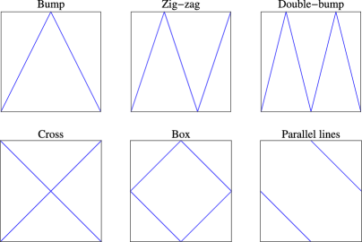
Figure 4: Simulations were done for data generated from the uniform distribution on the lines within each of the six boxes. For all except the Zig–zag and the Parallel lines, the ordinary correlation is zero.

In Figure 4, six boxes with lines in them are represented, and we simulated from the uniform distribution on these lines. The first five maximize or minimize the correlation between some simple orthogonal functions for given uniform marginals. In particular, say the boxes represent the square $[0,1]\times[0,1]$, then the Bump, Zig–zag and Double bump distributions maximize, for given uniform marginals,

$$\rho\bigl{[}\cos(2\uppi X),\cos(\uppi Y)\bigr{]},\qquad\rho\bigl{[}\cos(3\uppi X),\cos(\uppi Y)\bigr{]}\quad\mbox{and}\quad\rho\bigl{[}\cos(4\uppi X),\cos(\uppi Y)\bigr{]},$$

respectively. The Cross and Box distributions respectively maximize and minimize, for given uniform marginals,

$$\rho\bigl{[}\cos(2\uppi X),\cos(2\uppi Y)\bigr{]}.$$

As they represent in this sense extreme forms of association, these distributions should yield good insight in the comparative performance of the tests. Furthermore, the Parallel lines distribution was chosen because it is simple and demonstrates a weakness of Hoeffding’s test, as it has comparatively very little power here (we did not manage to find a distribution where $D$ or $\tau^{*}$ fare so comparatively poorly). Note that all six distributions have uniform marginals and so are copulas, and several were also discussed in Nelsen [18].

We also did a Bayesian simulation, based on random distributions with dependence. In particular, the data are $(X_{1},Y_{1}),\ldots,(X_{n},Y_{n})$, where, for i.i.d. $(\varepsilon_{1i},\varepsilon_{2i})$,

$$(X_{1},Y_{1}) = (\varepsilon_{11},\varepsilon_{21}),$$

$$(X_{i+1},Y_{i+1}) = (X_{i},Y_{i})+(\varepsilon_{1i},\varepsilon_{2i})\qquad i=1,\ldots,n-1.$$

Of course, the $(X_{i},Y_{i})$ are not i.i.d., but conditioning on the empirical marginals the permutations of the $Y$-values give equally likely data sets under the null hypothesis of independence, so the permutation test is valid. Two distributions for the increments $(\varepsilon_{1i},\varepsilon_{2i})$ were used: independent normals and independent Cauchy distributions. In Figure 5, points generated in this way are plotted. Note that for the Cauchy increments, the heavy tails of the marginal distributions are automatically taken care of by the use of ranks, so in that respect the three tests described here are particularly suitable.

Finally, we also simulated normally distributed data with correlation $0.5$.

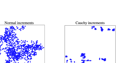
Figure 5: 1000 points of a random walk. In the first plot the $(x,y)$ increments are independent normals, in the second they are independent Cauchy variables.

Table 3: Average $p$-values. See Figures 4 and 5 and the text for explanations

		Average $p$-value
Distribution	Sample size $n$	$D$	$H$	$\tau^{*}$
Random walk (normal increments)	50	0.061	0.080	0.061
Random walk (Cauchy increments)	30	0.039	0.065	0.031
Bump	12	0.087	0.061	0.045
Zig–zag	25	0.083	0.011	0.036
Double-bump	30	0.056	0.005	0.019
Cross	50	0.052	0.003	0.021
Box	50	0.070	0.008	0.019
Parallel lines	10	0.055	0.710	0.076
Normal distribution ($\rho=0.5$)	30	0.055	0.052	0.073

Average $p$-values are given in Table 3, where all averages are over at least 40,000 simulations (for $D$, we did 200,000 simulations). Hoeffding’s test compares extremely badly with our test for the parallel lines distribution, and is worse than our test for the random walks, but outperforms our test for the Zig–zag, Double-bump, Cross and Box distributions. The reason for the poor performance of Hoeffding’s test for the parallel lines distribution is that five points can only be concordant (see Section 3.1) if they all lie on a single line (a discordant set of five points has zero probability). Similarly, for the Zig–zag, Double-bump and Cross concordant sets of five points can be seen to be especially likely, so these choices of distributions favour the Hoeffding test. Note that Hoeffding’s test is less suitable for general use because it is not necessarily zero under independence if there is a positive probability of tied observations.

The BKR test fares slightly worse than ours for the random walk with Cauchy increments, and significantly worse than ours for the Bump, Zig–zag, Cross and Box distributions, and does somewhat better than ours for the normal distribution. It appears that the BKR test has more power than ours for a monotone alternative (such as the normal distribution), at the cost of less power for some more complex alternatives.

5 Proof of Theorem 1

Here we give the proof of Theorem 1 for arbitrary real random variables $X$ and $Y$. A shorter proof for continuous $X$ and $Y$ is given by Dassios and Bergsma [3]. Readers wishing to gain an understanding of the essence of the proof may wish to study the shorter proof first.

First, consider three real valued random variables $U$, $V$and $W$. They have continuous densities $\tilde{f}(x)$, $\tilde{g}(x)$ and  $\tilde{k}(x)$ as well as probability masses $f(x_{i})$, $g(x_{i})$ and $k(x_{i})$ at points $x_{1},x_{2},\ldots.$ We also define

$$F(x) = P(U<x)=\sum_{x_{i}<x}f(x_{i})+\int_{y<x}\tilde{f}(y)\,\mathrm{d}y,$$

$$G(x) = P(V<x)=\sum_{x_{i}<x}g(x_{i})+\int_{y<x}\tilde{g}(y)\,\mathrm{d}y$$

and

$$K(x)=P(W<x)=\sum_{x_{i}<x}k(x_{i})+\int_{y<x}\tilde{k}(y)\,\mathrm{d}y.$$

We will also use $H(x)=\frac{K(x)}{G(x)}$. Note that $H(x)$ also admits the representation

$$H(x)=\sum_{x_{i}<x}h(x_{i})+\int_{y<x}\tilde{h}(y)\,\mathrm{d}y$$

but unlike the other three function that are non-decreasing $\tilde{h}(x)$ and $h(x_{i})$ can take negative values.

We start by proving the following intermediate result.

Lemma 1

Assume that $G(x)=1$ implies $F(x)=K(x)=1$ and that there is a constant $c$ such that $F(x)\leq cG(x)$ and $K(x)\leq cG^{2}(x)$ for all $x$. Define

$$S = 2\sum\bigl{(}F(x_{i})-G(x_{i})\bigr{)}\bigl{(}F(x_{i})g(x_{i})-G(x_{i})f(x_{i})\bigr{)}\frac{K(x_{i})}{G^{2}(x_{i})}$$

$${}-\sum\bigl{(}F(x_{i})g(x_{i})-G(x_{i})f(x_{i})\bigr{)}^{2}\frac{K(x_{i})}{G^{2}(x_{i})}$$

$${}+2\int\bigl{(}F(x)-G(x)\bigr{)}\bigl{(}F(x)\tilde{g}(x)-G(x)\tilde{f}(x)\bigr{)}\frac{K(x)}{G^{2}(x)}\,\mathrm{d}x,$$

where summation is over all $x_{i}$ such that $K(x_{i})>0$ and at least one of $f(x_{i})$ and $g(x_{i})$ is positive, and integration is over all $x$ such that $K(x)>0$.

We then have $S\geq 0$ with equality iff $F(x)=G(x)$ for all $x$ such that $K(x)>0$.

[Proof.] The conditions stated in the lemma ensure that the sums and integral exist. We can rewrite

$$S = 2\sum\bigl{(}F(x_{i})-G(x_{i})\bigr{)}\bigl{(}F(x_{i})g(x_{i})-G(x_{i})f(x_{i})\bigr{)}\frac{H(x_{i})}{G(x_{i})}$$

$${}-\sum\bigl{(}F(x_{i})g(x_{i})-G(x_{i})f(x_{i})\bigr{)}^{2}\frac{H(x_{i})}{G(x_{i})}$$

$${}+2\int\bigl{(}F(x)-G(x)\bigr{)}\bigl{(}F(x)\tilde{g}(x)-G(x)\tilde{f}(x)\bigr{)}\frac{H(x)}{G(x)}\,\mathrm{d}x.$$

For simplicity, we denote $F(x),G(x),H(x),f(x_{i}),g(x_{i}),h(x_{i}),\tilde{f}(x),\tilde{g}(x)$ and $\tilde{h}(x)$ by $F,G,H,f,g,h,\tilde{f},\tilde{g}$ and $\tilde{h}$. We have

$$S = 2\sum(F-G)\bigl{(}(F-G)g-G(f-g)\bigr{)}\frac{H}{G}$$

$${}+2\int(F-G)\bigl{(}(F-G)\tilde{g}-G(\tilde{f}-\tilde{g})\bigr{)}\frac{H}{G}\,\mathrm{d}x$$

$${}-\sum\bigl{(}(F-G)g-G(f-g)\bigr{)}^{2}\frac{H}{G}$$

$$= 2\sum(F-G)^{2}\frac{H}{G}g+2\int(F-G)^{2}\frac{H}{G}\tilde{g}\,\mathrm{d}x$$

$${}-2\sum H(F-G)(f-g)$$

$${}-2\int H(F-G)(\tilde{f}-\tilde{g})\,\mathrm{d}x$$

$${}-\sum\bigl{(}(F-G)g-G(f-g)\bigr{)}^{2}\frac{H}{G}.$$

The function $H(F-G)^{2}$ vanishes at $-\infty$ (because of the conditions of the lemma) and $+\infty$. Considering its integral and sum representation we have

$$2\sum H(F-G)(f-g)+2\int H(F-G)(\tilde{f}-\tilde{g})\,\mathrm{d}x$$

$$\quad{}+\sum(F-G)^{2}h+\int(F-G)^{2}\tilde{h}\,\mathrm{d}x$$

$$\quad{}+2\sum(F-G)(f-g)h+\sum(f-g)^{2}h+\sum H(f-g)^{2}=0,$$

and therefore

$$-2\sum H(F-G)(f-g)-2\int H(F-G)(\tilde{f}-\tilde{g})\,\mathrm{d}x$$

$$\quad=\sum(F-G)^{2}h+\int(F-G)^{2}\tilde{h}\,\mathrm{d}x$$ (13)

$$\qquad{}+2\sum(F-G)(f-g)h+\sum(f-g)^{2}h+\sum H(f-g)^{2}.$$

Moreover,

$$\frac{H}{G}\bigl{(}(F-G)g-G(f-g)\bigr{)}^{2}$$

(14)

$$\quad=(F-G)^{2}g^{2}\frac{H}{G}+GH(f-g)^{2}-2(F-G)(f-g)Hg.$$

Substituting (5)  and (5) into (5), and denoting $M=F-G$, $m=f-g$ and $\tilde{m}=\tilde{f}-\tilde{g}$ we have

$$S = \sum M^{2}\biggl{(}2g\frac{H}{G}+h-g^{2}\frac{H}{G}\biggr{)}+2\sum Mm(h+gH)+\sum m^{2}(H+h-GH)$$

$${}+\int M^{2}\biggl{(}2\tilde{g}\frac{H}{G}+\tilde{h}\biggr{)}\,\mathrm{d}x$$

$$= \sum(M+m)^{2}\biggl{(}g\frac{H}{G+g}+h\biggr{)}+\sum M^{2}\biggl{(}2g\frac{H}{G}-g\frac{H}{G+g}-g^{2}\frac{H}{G}\biggr{)}$$

$${}-2\sum Mm\biggl{(}g\frac{H}{G+g}-gH\biggr{)}+\sum m^{2}\biggl{(}H-GH-g\frac{H}{G+g}\biggr{)}$$

$${}+\int M^{2}\biggl{(}\tilde{g}\frac{H}{G}+\tilde{h}\biggr{)}\,\mathrm{d}x+\int M^{2}\tilde{g}\frac{H}{G}\,\mathrm{d}x$$

$$= \sum(M+m)^{2}\biggl{(}g\frac{H}{G+g}+h\biggr{)}+\int M^{2}\biggl{(}\tilde{g}\frac{H}{G}+\tilde{h}\biggr{)}\,\mathrm{d}x+\int M^{2}\tilde{g}\frac{H}{G}\,\mathrm{d}x$$

$${}+\sum M^{2}\biggl{(}g\frac{H}{G}+g^{2}\frac{H(1-G-g)}{G(G+g)}\biggr{)}-2\sum Mm\biggl{(}g\frac{H(1-G-g)}{G+g}\biggr{)}$$

$${}+\sum m^{2}\frac{H}{G+g}\bigl{(}(1-G)G-gG\bigr{)}.$$

Observe now that since $K=HG$

$$g\frac{H}{G+g}+h=\frac{gH+hG+hg}{G+g}=\frac{k}{G+g}\geq 0$$

and

$$\tilde{g}\frac{H}{G}+\tilde{h}=\frac{\tilde{k}}{G}\geq 0.$$

Moreover, the quadratic form

$$M^{2}\biggl{(}g\frac{H}{G}+g^{2}\frac{H(1-G-g)}{G(G+g)}\biggr{)}-2Mm\biggl{(}g\frac{H(1-G-g)}{G+g}\biggr{)}+m^{2}\frac{H}{G+g}\bigl{(}(1-G)G-gG\bigr{)}$$

$$\quad=\frac{M^{2}gH}{G}+(Mg-mG)^{2}\frac{H(1-G-g)}{G(G+g)}.$$

All terms in $S$ are non-negative and are equal to zero iff $M(x)=0$ for all $x$ such that $K(x)>0$, that is the two distributions $F$ and $G$ are identical for all $x$ such that $K(x)>0$.

Before we prove Theorem 1, we will prove another result as it will be used repeatedly.

Lemma 2

Let $A$, $B$ and $C$ be events in the same probability space as the random variable $X$ and define

$$L\bigl{(}x^{(1)},x^{(2)}\bigr{)} = \bigl{(}P\bigl{(}A|X=x^{(1)}\bigr{)}-P\bigl{(}A|X<x^{(1)}\wedge x^{(2)}\bigr{)}\bigr{)}$$

$${}\times\bigl{(}P\bigl{(}A|X=x^{(2)}\bigr{)}-P\bigl{(}A|X<x^{(1)}\wedge x^{(2)}\bigr{)}\bigr{)}$$

$${}\times P\bigl{(}B|X<x^{(1)}\wedge x^{(2)}\bigr{)}P\bigl{(}C|X<x^{(1)}\wedge x^{(2)}\bigr{)}\bigl{(}P\bigl{(}X<x^{(1)}\wedge x^{(2)}\bigr{)}\bigr{)}^{2}.$$

We then have

$$E\bigl{(}L(X_{1},X_{2})\bigr{)}\geq 0$$

with equality iff $P(X<x)=P(X<x|A)$  for all $x$ such that $P(X<x|B)P(X<x|C)>0$.

[Proof.] Let $X$ have continuous density $\tilde{g}(x)$ and probability masses $g(x_{i})$ at points $x_{1},x_{2},\ldots$ and let $X$ have continuous density $\tilde{g}_{A}(x)$ and probability masses $g_{A}(x_{i})$ at points $x_{1},x_{2},\ldots$ conditionally on $A$. Define also

$$G(x)=P(X<x)=\sum_{x_{i}<x}g(x_{i})+\int_{y<x}\tilde{g}(y)\,\mathrm{d}y$$

and

$$G_{A}(x)=P\bigl{(}X<x|A\bigr{)}=\sum_{x_{i}<x}g_{A}(x_{i})+\int_{y<x}\tilde{g}_{A}(y)\,\mathrm{d}y.$$

Conditioning on values of $X_{1}\wedge X_{2}$ and using Bayes’ theorem, we can see that

$$E\bigl{(}L(X_{1},X_{2})\bigr{)}$$

$$\quad=\bigl{(}P(A)\bigr{)}^{2}\sum P\bigl{(}B|X<x_{i}\bigr{)}P\bigl{(}C|X<x_{i}\bigr{)}$$

$$\qquad{}\times\bigl{\{}2\bigl{(}\bigl{(}1-G_{A}(x_{i})\bigr{)}G(x_{i})-\bigl{(}1-G(x_{i})\bigr{)}G_{A}(x_{i})\bigr{)}\bigl{(}g_{A}(x_{i})G(x_{i})-g(x_{i})G_{A}(x_{i})\bigr{)}$$

$$\hskip 15.0pt\qquad{}-\bigl{(}g_{A}(x_{i})G(x_{i})-g(x_{i})G_{A}(x_{i})\bigr{)}^{2}\bigr{\}}$$

$$\qquad{}+\bigl{(}P(A)\bigr{)}^{2}\int P\bigl{(}B|X<x\bigr{)}P\bigl{(}C|X<x\bigr{)}$$

$$\hskip 55.0pt\qquad{}\times 2\bigl{(}\bigl{(}1-G_{A}(x)\bigr{)}G(x)-\bigl{(}1-G(x)\bigr{)}G_{A}(x)\bigr{)}\bigl{(}\tilde{g}_{A}(x)G(x)-\tilde{g}(x)G_{A}(x)\bigr{)}\,\mathrm{d}x$$

$$\quad=P(B)P(C)\bigl{(}P(A)\bigr{)}^{2}\sum\frac{K(x_{i})}{G^{2}(x_{i})}\cdot\bigl{\{}2\bigl{(}G(x_{i})-G_{A}(x_{i})\bigr{)}\bigl{(}g_{A}(x_{i})G(x_{i})-g(x_{i})G_{A}(x_{i})\bigr{)}$$

$$\hskip 138.0pt\qquad{}-\bigl{(}g_{A}(x_{i})G(x_{i})-g(x_{i})G_{A}(x_{i})\bigr{)}^{2}\bigr{\}}$$

$$\qquad{}+P(B)P(C)\bigl{(}P(A)\bigr{)}^{2}\int\frac{K(x)}{G^{2}(x)}2\bigl{(}G(x)-G_{A}(x)\bigr{)}\bigl{(}\tilde{g}_{A}(x)G(x)-\tilde{g}(x)G_{A}(x)\bigr{)}\,\mathrm{d}x,$$

where

$$K(x)=P\bigl{(}X<x|B\bigr{)}P\bigl{(}X<x|C\bigr{)}.$$

The result then follows from Lemma 1 ($F=G_{A}$). It is easy to see that the conditions in Lemma 1 are satisfied. For example, $P(X<x|B)\leq\frac{P(X<x)}{P(B)}$.

Proof of Theorem 1 We need to prove that

$$P(Y_{1}\wedge Y_{2}>Y_{3}\vee Y_{4},X_{3}\vee X_{4}<X_{1}\wedge X_{2})$$

$$\quad{}+P(Y_{1}\vee Y_{2}<Y_{3}\wedge Y_{4},X_{3}\vee X_{4}<X_{1}\wedge X_{2})$$

$$\quad{}-P(Y_{1}\wedge Y_{3}>Y_{2}\vee Y_{4},X_{3}\vee X_{4}<X_{1}\wedge X_{2})$$

$$\quad{}-P(Y_{1}\vee Y_{3}<Y_{2}\wedge Y_{4},X_{3}\vee X_{4}<X_{1}\wedge X_{2})\geq 0$$

with equality in the independence case.

Let $(X,Y)$ represent any of the pairs $(X_{i,}Y_{i})$. Define now $F_{1}(y)=P(Y<y|X=x^{(1)})$,  $F_{2}(y)=P(Y<y|X=x^{(2)})$ and $G(y)=P(Y<y|X<x^{(1)}\wedge x^{(2)})$  with the representations

$$F_{1}(y) = \sum_{y_{i}<y}f_{1}(y_{i})+\int_{z<y}\widetilde{f}_{1}(z)\,\mathrm{d}z,$$

$$F_{2}(y) = \sum_{y_{i}<y}f_{2}(y_{i})+\int_{z<y}\widetilde{f}_{2}(z)\,\mathrm{d}z$$

and

$$G(y)=\sum_{y_{i}<y}g(y_{i})+\int_{z<y}\tilde{g}(z)\,\mathrm{d}z.$$

Note that conditionally on the event

$$\Theta=\bigl{\{}X_{1}=x^{(1)},X_{2}=x^{(2)},X_{3}<x^{(1)}\wedge x^{(2)},X_{4}<x^{(1)}\wedge x^{(2)}\bigr{\}},$$

the distribution of the minimum of $Y_{1}$ and $Y_{2}$ has density $(1-F_{1})\widetilde{f}_{2}+(1-F_{2})\widetilde{f}_{1}$ and probability masses $(1-F_{1})f_{2}+(1-F_{2})f_{1}-f_{1}f_{2}$ at $y_{1},y_{2},\ldots,$ the distribution of the minimum of  $Y_{3}$ and $Y_{4}$ has density $2(1-G)\tilde{g}$ and probability masses $2(1-G)g-g^{2}$, the  distribution of the minimum of $Y_{1}$ and $Y_{3}$ has density $(1-F_{1})\tilde{g}+(1-G)\widetilde{f}_{1}$ and probability masses $(1-F_{1})g+(1-G)f_{1}-f_{1}g$ and the distribution of the minimum of $Y_{2}$ and $Y_{4}$ has density $(1-F_{2})\tilde{g}+(1-G)\widetilde{f}_{2}$ and probability masses $(1-F_{2})g+(1-G)f_{2}-f_{2}g$. We therefore have (suppressing the arguments of the functions)

$$P\bigl{(}Y_{1}\wedge Y_{2}>Y_{3}\vee Y_{4}|\Theta\bigr{)}+P\bigl{(}Y_{1}\vee Y_{2}<Y_{3}\wedge Y_{4}|\Theta\bigr{)}$$

$$\qquad{}-P\bigl{(}Y_{1}\wedge Y_{3}>Y_{2}\vee Y_{4}|\Theta\bigr{)}-P\bigl{(}Y_{1}\vee Y_{3}<Y_{2}\wedge Y_{4}|\Theta\bigr{)}$$

$$\quad=\sum\bigl{(}(1-F_{1})f_{2}+(1-F_{2})f_{1}-f_{1}f_{2}\bigr{)}G^{2}+\sum\bigl{(}2(1-G)g-g^{2}\bigr{)}F_{1}F_{2}$$

$$\qquad{}-\sum\bigl{(}(1-F_{1})g+(1-G)f_{1}-f_{1}g\bigr{)}F_{2}G-\sum\bigl{(}(1-F_{2})g+(1-G)f_{2}-f_{2}g\bigr{)}F_{1}G$$

$$\qquad{}+\int\bigl{(}(1-F_{1})\widetilde{f}_{2}+(1-F_{2})\widetilde{f}_{1}\bigr{)}G^{2}\,\mathrm{d}y+\int 2(1-G)\tilde{g}F_{1}F_{2}\,\mathrm{d}y$$

$$\qquad{}-\int\bigl{(}(1-F_{1})\tilde{g}+(1-G)\widetilde{f}_{1}\bigr{)}F_{2}G\,\mathrm{d}y-\int\bigl{(}(1-F_{2})\tilde{g}+(1-G)\widetilde{f}_{2}\bigr{)}F_{1}G\,\mathrm{d}y$$

$$\quad=\sum(F_{1}-G)(F_{2}g-Gf_{2})+\sum(F_{2}-G)(F_{1}g-Gf_{1})-\sum(F_{1}g-Gf_{1})(F_{2}g-Gf_{2})$$

$$\qquad{}+\int(F_{1}-G)(F_{2}\tilde{g}-G\widetilde{f}_{2})\,\mathrm{d}y+\int(F_{2}-G)(F_{1}\tilde{g}-G\tilde{f}_{1})\,\mathrm{d}y$$

$$\quad=2\sum(F_{1}-G)(F_{2}-G)g-\sum(F_{1}-G)(f_{2}-g)G-\sum(F_{2}-G)(f_{1}-g)G$$

$$\qquad{}-\sum(F_{1}g-Gf_{1})(F_{2}g-Gf_{2})+2\int(F_{1}-G)(F_{2}-G)\tilde{g}\,\mathrm{d}y$$

$$\qquad{}-\int(F_{1}-G)(\tilde{f}_{2}-\tilde{g})G\,\mathrm{d}y-\int(F_{2}-G)(\tilde{f}_{1}-\tilde{g})G\,\mathrm{d}y.$$

The function $G(F_{1}-G)(F_{2}-G)$ vanishes at $-\infty$  and $+\infty$. Considering its integral and sum representation, we have

$$-\sum(F_{1}-G)(f_{2}-g)G-\sum(F_{2}-G)(f_{1}-g)G$$

$$\qquad{}-\int(F_{1}-G)(\tilde{f}_{2}-\tilde{g})G\,\mathrm{d}y-\int(F_{2}-G)(\tilde{f}_{1}-\tilde{g})G\,\mathrm{d}y$$

$$\quad=\sum(F_{1}-G)(F_{2}-G)g+\sum(F_{1}-G)(f_{2}-g)g+\sum(F_{2}-G)(f_{1}-g)g$$

$$\qquad{}+\sum(f_{1}-g)(f_{2}-g)G+\sum(f_{2}-g)(f_{1}-g)g$$

$$\qquad{}+\int(F_{1}-G)(F_{2}-G)\tilde{g}\,\mathrm{d}y$$

$$\quad=\sum(F_{1}+f_{1}-G-g)(F_{2}+f_{2}-G-g)g$$

$$\qquad{}+\sum(f_{1}-g)(f_{2}-g)G+\int(F_{1}-G)(F_{2}-G)\tilde{g}\,\mathrm{d}y.$$

Moreover,

$$(F_{1}g-Gf_{1})(F_{2}g-Gf_{2}) = (F_{1}-G)(F_{2}-G)g^{2}-(F_{1}-G)(f_{2}-g)Gg$$

$${}-(F_{2}-G)(f_{1}-g)Gg+(f_{1}-g)(f_{2}-g)G^{2}$$

$$= (F_{1}-G)(F_{2}-G)g^{2}+(f_{1}-g)(f_{2}-g)G^{2}$$

$${}-(F_{1}+f_{1}-G-g)(F_{2}+f_{2}-G-g)gG$$

$${}+(F_{1}-G)(F_{2}-G)gG+(f_{1}-g)(f_{2}-g)gG$$

$$= (F_{1}-G)(F_{2}-G)g(G+g)+(f_{1}-g)(f_{2}-g)G(G+g)$$

$${}-(F_{1}+f_{1}-G-g)(F_{2}+f_{2}-G-g)gG.$$

Using (5) and (5), we have

$$P\bigl{(}Y_{1}\wedge Y_{2}>Y_{3}\vee Y_{4}|\Theta\bigr{)}+P\bigl{(}Y_{1}\vee Y_{2}<Y_{3}\wedge Y_{4}|\Theta\bigr{)}$$

$$\qquad{}-P\bigl{(}Y_{1}\wedge Y_{3}>Y_{2}\vee Y_{4}|\Theta\bigr{)}-P\bigl{(}Y_{1}\vee Y_{3}<Y_{2}\wedge Y_{4}|\Theta\bigr{)}$$

$$\quad=\sum(F_{1}-G)(F_{2}-G)g+\sum(F_{1}-G)(F_{2}-G)g(1-G-g)$$

$$\qquad{}+\sum(F_{1}+f_{1}-G-g)(F_{2}+f_{2}-G-g)g$$

$$\qquad{}+\sum(F_{1}+f_{1}-G-g)(F_{2}+f_{2}-G-g)gG$$

$$\qquad{}+\sum(f_{1}-g)(f_{2}-g)G(1-G-g)+3\int(F_{1}-G)(F_{2}-G)\tilde{g}\,\mathrm{d}y.$$

We therefore conclude that conditionally on  $\{X_{1}=x^{(1)},X_{2}=x^{(2)}\}$,

$$P(Y_{1}\wedge Y_{2}>Y_{3}\vee Y_{4},X_{3}\vee X_{4}<X_{1}\wedge X_{2})$$

$$\qquad{}+P(Y_{1}\vee Y_{2}<Y_{3}\wedge Y_{4},X_{3}\vee X_{4}<X_{1}\wedge X_{2})$$

$$\qquad{}-P(Y_{1}\wedge Y_{3}>Y_{2}\vee Y_{4},X_{3}\vee X_{4}<X_{1}\wedge X_{2})$$

$$\qquad{}-P(Y_{1}\vee Y_{3}<Y_{2}\wedge Y_{4},X_{3}\vee X_{4}<X_{1}\wedge X_{2})$$

$$\quad=\sum\bigl{(}P\bigl{(}Y<y|X=x^{(1)}\bigr{)}-P\bigl{(}Y<y|X<x^{(1)}\wedge x^{(2)}\bigr{)}\bigr{)}$$

$$\quad\qquad{}\times\bigl{(}P\bigl{(}Y<y|X=x^{(2)}\bigr{)}-P\bigl{(}Y<y|X<x^{(1)}\wedge x^{(2)}\bigr{)}\bigr{)}$$

$$\quad\qquad{}\times P\bigl{(}Y=y|X<x^{(1)}\wedge x^{(2)}\bigr{)}\bigl{(}P\bigl{(}X<x^{(1)}\wedge x^{(2)}\bigr{)}\bigr{)}^{2}$$

$$\qquad{}+\sum\bigl{(}P\bigl{(}Y<y|X=x^{(1)}\bigr{)}-P\bigl{(}Y<y|X<x^{(1)}\wedge x^{(2)}\bigr{)}\bigr{)}$$

$$\hskip 5.0pt\qquad\qquad{}\times\bigl{(}P\bigl{(}Y<y|X=x^{(2)}\bigr{)}-P\bigl{(}Y<y|X<x^{(1)}\wedge x^{(2)}\bigr{)}\bigr{)}$$

$$\hskip 5.0pt\qquad\qquad{}\times P\bigl{(}Y=y|X<x^{(1)}\wedge x^{(2)}\bigr{)}P\bigl{(}Y>y|X<x^{(1)}\wedge x^{(2)}\bigr{)}\bigl{(}P\bigl{(}X<x^{(1)}\wedge x^{(2)}\bigr{)}\bigr{)}^{2}$$

$$\qquad{}+\sum\bigl{(}P\bigl{(}Y\leq y|X=x^{(1)}\bigr{)}-P\bigl{(}Y\leq y|X<x^{(1)}\wedge x^{(2)}\bigr{)}\bigr{)}$$

$$\hskip 5.0pt\qquad\qquad{}\times\bigl{(}P\bigl{(}Y\leq y|X=x^{(2)}\bigr{)}-P\bigl{(}Y\leq y|X<x^{(1)}\wedge x^{(2)}\bigr{)}\bigr{)}$$

$$\hskip 5.0pt\qquad\qquad{}\times P\bigl{(}Y=y|X<x^{(1)}\wedge x^{(2)}\bigr{)}\bigl{(}P\bigl{(}X<x^{(1)}\wedge x^{(2)}\bigr{)}\bigr{)}^{2}$$

$$\qquad{}+\sum\bigl{(}P\bigl{(}Y\leq y|X=x^{(1)}\bigr{)}-P\bigl{(}Y\leq y|X<x^{(1)}\wedge x^{(2)}\bigr{)}\bigr{)}$$

$$\hskip 5.0pt\qquad\qquad{}\times\bigl{(}P\bigl{(}Y\leq y|X=x^{(2)}\bigr{)}-P\bigl{(}Y\leq y|X<x^{(1)}\wedge x^{(2)}\bigr{)}\bigr{)}$$

$$\hskip 5.0pt\qquad\qquad{}\times P\bigl{(}Y=y|X<x^{(1)}\wedge x^{(2)}\bigr{)}P\bigl{(}Y<y|X<x^{(1)}\wedge x^{(2)}\bigr{)}\bigl{(}P\bigl{(}X<x^{(1)}\wedge x^{(2)}\bigr{)}\bigr{)}^{2}$$

$$\qquad{}+\sum\bigl{(}P\bigl{(}Y=y|X=x^{(1)}\bigr{)}-P\bigl{(}Y=y|X<x^{(1)}\wedge x^{(2)}\bigr{)}\bigr{)}$$

$$\hskip 5.0pt\qquad\qquad{}\times\bigl{(}P\bigl{(}Y=y|X=x^{(2)}\bigr{)}-P\bigl{(}Y=y|X<x^{(1)}\wedge x^{(2)}\bigr{)}\bigr{)}$$

$$\hskip 5.0pt\qquad\qquad{}\times P\bigl{(}Y<y|X<x^{(1)}\wedge x^{(2)}\bigr{)}P\bigl{(}Y>y|X<x^{(1)}\wedge x^{(2)}\bigr{)}\bigl{(}P\bigl{(}X<x^{(1)}\wedge x^{(2)}\bigr{)}\bigr{)}^{2}$$

$$\qquad{}+3\int\bigl{(}P\bigl{(}Y<y|X=x^{(1)}\bigr{)}-P\bigl{(}Y<y|X<x^{(1)}\wedge x^{(2)}\bigr{)}\bigr{)}$$

$$\hskip 5.0pt\qquad\qquad{}\times\bigl{(}P\bigl{(}Y<y|X=x^{(2)}\bigr{)}-P\bigl{(}Y<y|X<x^{(1)}\wedge x^{(2)}\bigr{)}\bigr{)}$$

$$\hskip 5.0pt\qquad\qquad{}\times P\bigl{(}Y\in\,\mathrm{d}y|X<x^{(1)}\wedge x^{(2)}\bigr{)}\bigl{(}P\bigl{(}X<x^{(1)}\wedge x^{(2)}\bigr{)}\bigr{)}^{2}.$$

All of the above terms lead to non-negative expressions because of Lemma 2 (for the first, third and sixth term we take $C=\Omega$, the set of all possible outcomes). We then see that the expression can be zero iff $X$ and $Y$ are independent. The condition stated in Theorem 1 is needed to avoid complications when integrating over $x^{(1)}$ in the application of Lemma 2 to terms such as $\sum P(Y=y|X=x^{(1)})$.

References

• [1] {bbook}[mr] \bauthor\bsnmAgresti, \bfnmAlan\binitsA. (\byear2010). \btitleAnalysis of Ordinal Categorical Data, \bedition2nd ed. \bseriesWiley Series in Probability and Statistics. \blocationHoboken, NJ: \bpublisherWiley. \bidmr=2742515 \bptokimsref \endbibitem
• [2] {bmisc}[auto:STB—2013/05/03—14:24:43] \bauthor\bsnmBergsma, \bfnmW. P.\binitsW.P. (\byear2006). \bhowpublishedA new correlation coefficient, its orthogonal decomposition, and associated tests of independence. Available at \arxivurlarXiv:math/0604627v1 [math.ST]. \bptokimsref \endbibitem
• [3] {bmisc}[auto:STB—2013/05/03—14:24:43] \bauthor\bsnmBergsma, \bfnmW.\binitsW. &\bauthor\bsnmDassios, \bfnmA.\binitsA. (\byear2014). \bhowpublishedSupplement to “A consistent test of independence based on a sign covariance related to Kendall’s tau.” DOI:\doiurl10.3150/13-BEJ514SUPP. \bptokimsref \endbibitem
• [4] {barticle}[mr] \bauthor\bsnmBlum, \bfnmJ. R.\binitsJ.R., \bauthor\bsnmKiefer, \bfnmJ.\binitsJ. &\bauthor\bsnmRosenblatt, \bfnmM.\binitsM. (\byear1961). \btitleDistribution free tests of independence based on the sample distribution function. \bjournalAnn. Math. Statist. \bvolume32 \bpages485–498. \bidissn=0003-4851, mr=0125690 \bptokimsref \endbibitem
• [5] {barticle}[mr] \bauthor\bparticlede \bsnmWet, \bfnmT.\binitsT. (\byear1980). \btitleCramér–von Mises tests for independence. \bjournalJ. Multivariate Anal. \bvolume10 \bpages38–50. \biddoi=10.1016/0047-259X(80)90080-9, issn=0047-259X, mr=0569795 \bptokimsref \endbibitem
• [6] {barticle}[mr] \bauthor\bsnmDeheuvels, \bfnmPaul\binitsP. (\byear1981). \btitleAn asymptotic decomposition for multivariate distribution-free tests of independence. \bjournalJ. Multivariate Anal. \bvolume11 \bpages102–113. \biddoi=10.1016/0047-259X(81)90136-6, issn=0047-259X, mr=0612295 \bptokimsref \endbibitem
• [7] {barticle}[mr] \bauthor\bsnmEscoufier, \bfnmYves\binitsY. (\byear1973). \btitleLe traitement des variables vectorielles. \bjournalBiometrics \bvolume29 \bpages751–760. \bidissn=0006-341X, mr=0334416 \bptokimsref \endbibitem
• [8] {barticle}[auto:STB—2013/05/03—14:24:43] \bauthor\bsnmFeuerverger, \bfnmA.\binitsA. (\byear1993). \btitleA consistent test for bivariate dependence. \bjournalInternational Statistical Review/Revue Internationale de Statistique \bvolume61 \bpages419–433. \bptokimsref \endbibitem
• [9] {bincollection}[mr] \bauthor\bsnmGretton, \bfnmArthur\binitsA., \bauthor\bsnmBousquet, \bfnmOlivier\binitsO., \bauthor\bsnmSmola, \bfnmAlex\binitsA. &\bauthor\bsnmSchölkopf, \bfnmBernhard\binitsB. (\byear2005). \btitleMeasuring statistical dependence with Hilbert–Schmidt norms. In \bbooktitleAlgorithmic Learning Theory. \bseriesLecture Notes in Computer Science \bvolume3734 \bpages63–77. \blocationBerlin: \bpublisherSpringer. \biddoi=10.1007/11564089_7, mr=2255909 \bptokimsref \endbibitem
• [10] {bmisc}[mr] \bauthor\bsnmHeller, \bfnmR.\binitsR., \bauthor\bsnmHeller, \bfnmY.\binitsY. &\bauthor\bsnmGorfine, \bfnmM.\binitsM. (\byear2012). \bhowpublishedA consistent multivariate test of association based on ranks of distances. Available at \arxivurlarXiv:1201.3522. \bptokimsref \endbibitem
• [11] {barticle}[mr] \bauthor\bsnmHoeffding, \bfnmWassily\binitsW. (\byear1948). \btitleA non-parametric test of independence. \bjournalAnn. Math. Statistics \bvolume19 \bpages546–557. \bidissn=0003-4851, mr=0029139 \bptokimsref \endbibitem
• [12] {bbook}[mr] \bauthor\bsnmHollander, \bfnmMyles\binitsM. &\bauthor\bsnmWolfe, \bfnmDouglas A.\binitsD.A. (\byear1999). \btitleNonparametric Statistical Methods, \bedition2nd ed. \bseriesWiley Series in Probability and Statistics: Texts and References Section. \blocationNew York: \bpublisherWiley. \bidmr=1666064 \bptokimsref \endbibitem
• [13] {bbook}[mr] \bauthor\bsnmKendall, \bfnmMaurice\binitsM. &\bauthor\bsnmGibbons, \bfnmJean Dickinson\binitsJ.D. (\byear1990). \btitleRank Correlation Methods, \bedition5th ed. \bseriesA Charles Griffin Title. \blocationLondon: \bpublisherEdward Arnold. \bidmr=1079065 \bptokimsref \endbibitem
• [14] {barticle}[auto:STB—2013/05/03—14:24:43] \bauthor\bsnmKendall, \bfnmM. G.\binitsM.G. (\byear1938). \btitleA new measure of rank correlation. \bjournalBiometrika \bvolume30 \bpages81–93. \bptokimsref \endbibitem
• [15] {barticle}[mr] \bauthor\bsnmKimeldorf, \bfnmGeorge\binitsG. &\bauthor\bsnmSampson, \bfnmAllan R.\binitsA.R. (\byear1978). \btitleMonotone dependence. \bjournalAnn. Statist. \bvolume6 \bpages895–903. \bidissn=0090-5364, mr=0491562 \bptokimsref \endbibitem
• [16] {barticle}[mr] \bauthor\bsnmKruskal, \bfnmWilliam H.\binitsW.H. (\byear1958). \btitleOrdinal measures of association. \bjournalJ. Amer. Statist. Assoc. \bvolume53 \bpages814–861. \bidissn=0162-1459, mr=0100941 \bptokimsref \endbibitem
• [17] {barticle}[auto:STB—2013/05/03—14:24:43] \bauthor\bsnmLyons, \bfnmR.\binitsR. (\byear2013). \btitleDistance covariance in metric spaces. \bjournalAnn. Probab. \bvolume41 \bpages3284–3305. \bptokimsref \endbibitem
• [18] {bbook}[mr] \bauthor\bsnmNelsen, \bfnmRoger B.\binitsR.B. (\byear2006). \btitleAn Introduction to Copulas, \bedition2nd ed. \bseriesSpringer Series in Statistics. \blocationNew York: \bpublisherSpringer. \bidmr=2197664 \bptokimsref \endbibitem
• [19] {barticle}[mr] \bauthor\bsnmRényi, \bfnmA.\binitsA. (\byear1959). \btitleOn measures of dependence. \bjournalActa Math. Acad. Sci. Hungar. \bvolume10 \bpages441–451. \bidissn=0001-5954, mr=0115203 \bptokimsref \endbibitem
• [20] {barticle}[mr] \bauthor\bsnmRobert, \bfnmP.\binitsP. &\bauthor\bsnmEscoufier, \bfnmY.\binitsY. (\byear1976). \btitleA unifying tool for linear multivariate statistical methods: The $RV$-coefficient. \bjournalJ. R. Stat. Soc. Ser. C. Appl. Stat. \bvolume25 \bpages257–265. \bidissn=0035-9254, mr=0440801 \bptokimsref \endbibitem
• [21] {barticle}[mr] \bauthor\bsnmSchweizer, \bfnmB.\binitsB. &\bauthor\bsnmWolff, \bfnmE. F.\binitsE.F. (\byear1981). \btitleOn nonparametric measures of dependence for random variables. \bjournalAnn. Statist. \bvolume9 \bpages879–885. \bidissn=0090-5364, mr=0619291 \bptokimsref \endbibitem
• [22] {bincollection}[auto:STB—2013/05/03—14:24:43] \bauthor\bsnmSejdinovic, \bfnmD.\binitsD., \bauthor\bsnmGretton, \bfnmA.\binitsA., \bauthor\bsnmSriperumbudur, \bfnmB.\binitsB. &\bauthor\bsnmFukumizu, \bfnmK.\binitsK. (\byear2012). \btitleHypothesis testing using pairwise distances and associated kernels. In \bbooktitleProc. International Conference on Machine Learning. \blocationEdinburgh, UK: \bpublisherICML. \bptokimsref \endbibitem
• [23] {bmisc}[auto:STB—2013/05/03—14:24:43] \bauthor\bsnmSejdinovic, \bfnmD.\binitsD., \bauthor\bsnmSriperumbudur, \bfnmB.\binitsB., \bauthor\bsnmGretton, \bfnmA.\binitsA. &\bauthor\bsnmFukumizu, \bfnmK.\binitsK. (\byear2012). \bhowpublishedEquivalence of distance-based and RKHS-based statistics in hypothesis testing. Available at \arxivurlarXiv:1207.6076. \bptokimsref \endbibitem
• [24] {bbook}[mr] \bauthor\bsnmSheskin, \bfnmDavid J.\binitsD.J. (\byear2007). \btitleHandbook of Parametric and Nonparametric Statistical Procedures, \bedition4th ed. \blocationBoca Raton, FL: \bpublisherChapman & Hall/CRC. \bidmr=2296053 \bptokimsref \endbibitem
• [25] {barticle}[auto:STB—2013/05/03—14:24:43] \bauthor\bsnmSpearman, \bfnmC.\binitsC. (\byear1904). \btitleThe proof and measurement of association between two things. \bjournalThe American Journal of Psychology \bvolume15 \bpages72–101. \bptokimsref \endbibitem
• [26] {barticle}[mr] \bauthor\bsnmSzékely, \bfnmGábor J.\binitsG.J., \bauthor\bsnmRizzo, \bfnmMaria L.\binitsM.L. &\bauthor\bsnmBakirov, \bfnmNail K.\binitsN.K. (\byear2007). \btitleMeasuring and testing dependence by correlation of distances. \bjournalAnn. Statist. \bvolume35 \bpages2769–2794. \biddoi=10.1214/009053607000000505, issn=0090-5364, mr=2382665 \bptokimsref \endbibitem
• [27] {barticle}[mr] \bauthor\bsnmWilding, \bfnmGregory E.\binitsG.E. &\bauthor\bsnmMudholkar, \bfnmGovind S.\binitsG.S. (\byear2008). \btitleEmpirical approximations for Hoeffding’s test of bivariate independence using two Weibull extensions. \bjournalStat. Methodol. \bvolume5 \bpages160–170. \biddoi=10.1016/j.stamet.2007.07.002, issn=1572-3127, mr=2424751 \bptokimsref \endbibitem