11email: sewende@astro.physik.uni-goettingen.de 11email: Ansgar.Reiners@phys.uni-goettingen.de 22institutetext: Physics Department Univ. of California, One Shields Avenue Davis, CA 95616 USA
22email: seifahrt@physics.ucdavis.edu 33institutetext: Department of Chemistry, University of York, Heslington, York, YO10 5DD, UK
33email: pfb500@york.ac.uk
CRIRES spectroscopy and empirical line-by-line identification of FeH molecular absorption in an M dwarf††thanks: Data were taken at ESO Telescopes under the program 79.D-0357(A)
Molecular FeH provides a large number of sharp and isolated absorption lines that can be used to measure radial velocity, rotation, or magnetic field strength with high accuracy. Our aim is to provide an atlas for M-type stars in the spectral region from nm to nm (Wing-Ford band). To identify these lines in CRIRES spectra of the magnetically inactive, slowly rotating, M5.5 dwarf GJ1002, we calculated model spectra for the selected spectral region with theoretical line data. In general this line list agrees with the observed data, but several individual lines differ significantly in position or in line strength. After identification of as many as possible lines, we correct the line data for position and line strength to provide an accurate atlas of absorption lines for use in high precision spectroscopy of low mass stars. For all lines, we use a Voigt function to obtain their positions and equivalent widths. Identification with theoretical lines is done by hand. For confirmation of the identified lines, we use statistical methods, cross-correlation techniques, and line intensities. Eventually, we were able to identify lines from the , , , , , , and vibrational bands in the observed spectra and correct the positions of the lines if necessary. The deviations between theoretical and observed positions follow a normal distribution approximately around zero. In order to empirically correct the line strength, we determined , instrumental broadening (rotational broadening) and a van der Waals enhancement factor for lines in GJ1002. We also give scaling factors for the Einstein A values to correct the line strengths. With the identified lines, we derived rotational temperatures from line intensities for GJ1002. We conclude that lines can be used for a wide variety of applications in astrophysics. With the identified lines it will be possible for example to characterize magnetically sensitive or very temperature sensitive lines, which can be used to investigate M-type stars.
Key Words.:
Molecular data - line: identification, profiles - stars: low-mass1 Introduction
High resolution spectroscopy of atomic or molecular lines is used to measure rotation, magnetic fields, and radial velocity variations. In solar-like stars, atomic lines are useful to measure these quantities since they are numerous, well isolated and sufficiently narrow. In cooler stars, like M dwarfs, atomic lines are no longer useful because most of them become very weak, others become strongly pressure broadened and they are usually overlapped by strong molecular bands. In these stars molecular lines are a valuable tool to measure the quantities mentioned above. However, molecular lines tend to cluster in dense bands e.g. for and in the visual spectral range. Only a few molecules provide absorption lines that are isolated and can be used for detailed spectroscopic analysis.
The molecule provides a particularly large number of strong and well isolated lines in the z-band (– nm). It is the main opacity contributor in this region for late-type dwarf stars, and can be used for high precision spectroscopy. provides numerous unblended lines that are sufficiently narrow to measure small broadening effects or variations in the line position.
Wing & Ford (1969) first discovered the molecular band around nm in the spectra of the cool dwarf Wolf 359. This band was also found in S-type stars (Wing, 1972) and was identified as the vibrational band of the molecule by Nordh et al. (1977). An extensive analysis was carried out by Phillips et al. (1987). They identified seven vibrational bands of the electronic transition of the molecule and provided tables with molecular constants and quantum numbers. An important theoretical work, partly based on the previous one, was carried out by Dulick et al. (2003). They computed a line list for the electronic transition and provided large tables of molecular data with quantum numbers and line intensities.
absorption bands were also detected in the - and -band with medium resolution spectra (Cushing et al., 2003). In the -band the electronic transition is visible (Hargreaves et al., 2010). That can be used to determine effective temperatures was shown for example by Schiavon et al. (1997) or Wende et al. (2009), and its potential to measure magnetic field strengths was demonstrated by Reiners & Basri (2006, 2007). Theoretical work on the magnetic sensitivity of was published by Afram et al. (2007, 2008).
In this paper we use high resolution spectra of GJ1002 to empirically verify the line list of Dulick et al. (2003) and identify on a line-by-line basis in the region nm. For this purpose we will use Voigt functions to determine the empirical positions and equivalent widths of the observed lines. We identify the observed lines with theoretical ones by hand, and confirm this identification using statistical means, cross-correlation techniques, and the line strength of the identified lines. Furthermore, we correct theoretical Einstein A values to account for mismatches in line depth. We also derive rotational temperatures from the identified lines, and investigate under which circumstances they are close to the effective temperature of the star.
2 Data
2.1 CRIRES spectra of GJ1002
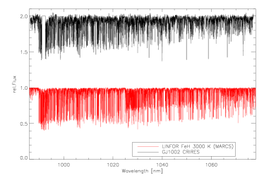
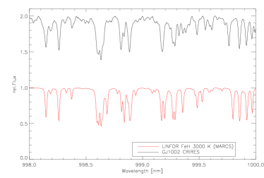
The observational data are CRIRES spectra of the inactive M 5.5 dwarf GJ1002 (see Fig. 1). The M dwarf has an assumed effective temperature of K (from the spectral type), and it is a very slow rotator ( km s-1, Reiners & Basri, 2007). There is also very low and X-ray activity from which we can assume that the magnetic field strength is relatively low. Due to the weak magnetic field and slow rotation, GJ1002 is an ideal target for identification of molecular lines. The lines are only slightly broadened by the different possible mechanisms in contrast to observations in sun spots where lines are always influenced by a strong magnetic field.
CRIRES observations of GJ1002 were conducted in service mode during several nights in July 2007. The entrance slit width was set to 0.2″, hence, the nominal resolving power was . Four frames with an integration time of five minutes were taken in an ABBA nod pattern for each of the nine wavelength settings covering the region between – nm, leaving only one larger gap at – nm and two smaller gaps at – nm and – nm.
Data reduction made use of the ESOREX pipeline for CRIRES. Science frames and flatfield frames were corrected for non-linearity and 1D spectra were extracted from the individual flatfielded and sky subtracted frames using an optimum extraction algorithm. The wavelength solution is based at first order on the Th-Ar calibration frames provided by ESO. Due to the slit curvature, spectra taken in B nodding positions are shifted in wavelength with respect to spectra taken in A nodding positions. This was corrected for by mapping all 1D spectra to the spectrum of the first A nod position.
The individual CRIRES wavelength settings provide a considerable degree of spectral overlap and up to eight individual spectra were combined to one final spectrum at each wavelength. While merging the individual settings, small mismatches in the wavelength solutions as well as imperfections in the individual spectra (detector cosmetics, ghost contamination) were corrected. The final spectrum was normalized to a pseudo-continuum level of unity and finally shifted to match the McMath FTS spectrum of solar umbra (Wallace et al., 1998). The error in the wavelength calibration should be smaller than km s-1.
We find the SNR at the continuum level of most parts of the final spectrum to exceed . The high signal-to-noise ratio and high spectral resolution of the CRIRES data allow us to identify lines with high accuracy.
2.2 Theoretical molecular data and line synthesis
The theoretical data which we use to identify the lines is taken from Dulick et al. (2003). They provide tables of quantum numbers and energies111See http://bernath.uwaterloo.ca/FeH. In particular, they provide the vibrational assignment of the upper and lower states and , respectively, the projection of the total orbital angular momentum on to the internuclear axis for the upper and lower state, and , and the rotational quantum number for the lower state. Furthermore the transition branch (P, Q, R), the parity, the wavenumber in cm-1, the lower state energy of the transition and the Einstein A value are given.
From this information it is possible to estimate -values through (Bernath, 2005)
| (1) |
with and as the lower and upper statistical weights of the transition and as the transition frequency. All quantities are in SI units.
The van der Waals broadening is determined following Schweitzer et al. (1996) which is basically Unsöld’s hydrogenic approximation. For the ionization energy needed in this approximation we use an empirically determined value of eV which was deduced from comparison with other diatomic molecules (Wende et al., 2009). Despite the fact that this is not the theoretical value, which is slightly higher, we use this one since its influence on the van der Waals broadening is not significant.
The molecular partition function for , which is needed for the concentration of is computed after Sauval & Tatum (1984) with molecular data taken from Tables 9 and 10 of Dulick et al. (2003). We give in equation 2 a polynomial expression of a fit to the partition function which is valid between K and K.
| (2) |
where is the temperature in K and
| (13) |
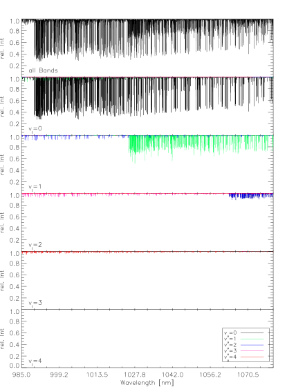
are the coefficients of the polynomial. For the creation of i.e. the concentration, which is governed by the Saha-Boltzmann equation, we assume . With this partition function and the data from Dulick et al. (2003), we can use a simple description for the absorbance (described in section 3.4 in this paper in more detail) to compute spectra with a simple reversing layer model and separate the lines into vibrational bands in the observed wavelength region (see Fig. 2). From this figure we can expect that there will be two sequences of vibrational transitions present. The sequence with , which are the , , and vibrational transitions, and the sequence with , which are the , , , and transitions. We note that this method does not take into account (among many other things) the atmospheric structure or the chemical composition of the star. It gives only a rough estimate of the relative strengths of the bands.
The full synthetic line formation for the comparison and identification of the observed lines is done with the line formation code SYNTH3 (Kochukhov, 2007). This code is able to compute large spectral regions with all lines taken from our line list (see Fig. 1). We use only lines with because we assume that other lines have no significant influence. By computing all the lines in a certain region at once, we account for blends, but we also compute all lines of the region individually in order to measure their equivalent width using the LINFOR3D code (based on Baschek et al., 1966). For the input model atmospheres we use MARCS (Gustafsson et al., 2008) with solar composition (Grevesse et al., 2007). These models are well suited for these cool temperatures in low mass stars, since they make use of up-to-date atomic and molecular data and go down to effective temperatures of K. We use the plane-parallel, LTE models where the convection is treated in the mixing-length approximation. In the computation of these model atmospheres, the microturbulence parameter was set to zero. However, in the computations of the actual spectra, we assume microturbulence parameters according to the results of Wende et al. (2009). We do not expect any significant influence since they are on the order of a few hundred m s-1. We neglect the broadening from macro-turbulent motion, which would be hardly visible in the observed spectra.
3 Methods
We start with the investigation of the observed spectrum, for which we determine the position of the spectral lines and decide whether a line feature is a blend or not. Then we measure the equivalent width of the lines with a Voigt fit procedure described below.
We compare the line positions found in the CRIRES data to theoretical ones and identify them with lines. In order to confirm an identification, we use statistical means: (i) the method of coincidence, and a cross-correlation technique producing coincidence curves; and (ii) a method which takes the intensity into account. In this latter method we will compare theoretical line strength (Hönl-London factor) with observed following Schadee (1964). We also use a description for the absorbance of spectral lines in order to correct theoretical line intensities given in terms of the Einstein A values. For this we will compare observed and computed spectra with each other and obtain a scaling factor for the Einstein A values. The final result is a corrected line list that reproduces the observed stellar spectrum as well as the line positions in sunspot spectra from Wallace et al. (1999). The line intensities are hard to confirm in the solar case, since many lines are strongly split by magnetic fields.
3.1 Voigt Fit
In order to measure in the observed spectra we use a ‘multi-Voigt fit’ procedure (based on IDL curvefit function). The ‘multi-Voigt fit’ is defined as
| (14) |
where A is the amplitude describing the depth of the line,
| (15) |
with as Gaussian (or Doppler) width,
| (16) |
which will be called the Voigt constant throughout in this paper, is the radiation damping constant, and is the Hjerting function (Gray, 2008, and references therein). We successively fit the whole spectrum within bins of Å . The first and the last Å are cut off after the fit to avoid boundary effects and we use only line profiles whose centers are inside the Å bin. For the Voigt profiles inside a bin, we assume a constant -value for the Lorentz part and a fixed Gaussian width, but we allow changes in these two parameters from one wavelength bin to another because the lines tend to become narrower towards longer wavelengths. This is probably because we use and only as fit parameters, and lines starts to saturate at the band head, but become weaker towards longer wavelengths. Hence, the width of the line profile, which is a combination of and decreases with decreasing saturation and so both parameters decrease. The wavelength dependence of the Doppler width affects the width of the lines as well, but it is negligible and goes in opposite direction (for example, Å at Å would change to Å at Å ).
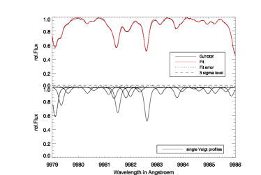
With this fit procedure, we obtain the parameters (position, depth (amplitude), Voigt constant, and ), needed for the individual Voigt line profiles to fit the observed spectrum. In Fig. 3, we show an example of how the fit (red) reduced the observed spectrum (black) into single line profiles (bottom panel).
The convergence criterion is the minimization of the residual flux between observation and fit (). The iteration is stopped if the maximal error of the fit is lower than three times the standard deviation of the error or if the standard deviation of the error does not change significantly between two iterations. From these Voigt profiles, can easily be computed by integrating over the single line profiles. The fit is also able to find and separate possible blends. For this, we assume that the blended components differ in position by at least Å .
The measured will be assigned to the associated theoretical lines. This means if an observed line can be identified with exactly one theoretical line, is fully assigned to this one theoretical line. However, in most cases theory predicts more than one line for an observed line position because of numerous overlapping vibrational bands in the same wavelength region and from many closely-spaced line pairs which only differ in parity. In these cases, will be distributed to all predicted theoretical lines at this position. This is done using the ratio of theoretical equivalent widths obtained from the individual theoretical line profiles:
| (17) |
with as the set of blended components. There is of course the chance that is not the only contributor to the observed blend. To avoid this uncertainty, we additionally use the line intensities in a method described below.
3.2 Method of coincidence
In order to confirm the identification of a molecular band, or a sub-band, we use the ‘method of coincidence’, which was first introduced by Russell & Bowen (1929). It gives the number of lines in a spectral range that will be found by chance if one uses a set of randomly generated line positions and compare them with observed ones. Fundamental probability calculations lead to
| (18) |
where is the number of lines in a particular region, is the tolerated deviation in position, and is the line density (average number of spectral lines in the investigated region). This means that gives the probability of finding, with a randomly chosen line position, a random coincidence. If one identifies out of lines in the observations, then the probability of finding an identification is . The ratio describes how likely it is to find per identified line a line by random coincidence. Hence, the number of actually identified lines should exceed the number of of purely random coincidences. If this is the case, then one can assume that the lines are probably identified in the observed spectra.
3.3 Theoretical Line Strength
For the identification of molecular lines, it is also useful to take the intensities of the lines into account. In order to compare the theoretical line strength with the observed equivalent width , we follow Schadee (1964). For weak lines (mildly saturated) is proportional to the wavelength , the oscillator strength , and , the number of absorbers (Gray, 2008):
| (19) |
and
| (20) |
with as the number of absorbers given by the Boltzmann distribution
| (21) |
where is the lower state energy level in cm-1. In order to derive the final form, we use equation 20 and 21 together with equation 19 and the expression for the Einstein A value
| (22) |
Here is the Einstein for a specific vibrational transition and constant for the vibrational band. The resulting equation is
| (23) |
which is the relation from Schadee (1964) with replacing . Possible stimulated emission can be neglected for our analysis since there is only a small population in the excited state. If we plot against , a straight line should be found, which then suggests the correct identification of the lines in the molecular band.

Equation 23 accounts for different branches as well as for different . This is because on the left side of equation 23 is computed for all branches (P, Q, R) and values.
The values that we will use in the analysis are computed for the intermediate Hund’s case and are determined from the Einstein values given by Dulick et al. (2003).
We point out that we implicitly assumed in equation 21 that the total number of molecules is constant for all lines. This assumption is only valid if we consider a small isothermal atmospheric layer. However, since a spectral line forms over several layers, this assumption is not exactly valid. If we furthermore consider a set of lines, with a wide range in and values, then we expect that these lines form at different heights. Thus, the number of molecules is not constant anymore: strong spectral lines are assumed to be formed in higher atmospheric layers, and weak lines in deeper layers. Hence, deviations from a straight line in the diagram for lines with very small and very high are expected. Assuming more molecules in deeper layers, due to higher density, larger equivalent widths for these lines can be expected. For a qualitative description, we assume the total number of molecules to be inversely proportional to the equivalent width, which reflects the heights of formation for weak and strong lines.
| (24) |
and are free parameters and here chosen as and , respectively. We plot the right hand side of equation 23 for constant and variable molecule number in Fig. 4. However, the situation is much more complicated and we use synthetic line formation to investigate this behavior in the results section.
Following Schadee (1964), we can now use the diagram to classify the identified lines into one of the following classes:
-
1.
P - the line is present, and its agrees well with the straight line of the diagram.
-
2.
Pb - the line is present, but its is too large, i.e. the value lies above the straight line of the diagram. This could imply that the line is blended by an other element (or that its computed line strength is too small).
-
3.
R - the line strength is presumably reduced by perturbations. That means, that the computed line strength is too large, and the data point lies below the line.
-
4.
Q - we identified the line, but we can’t verify its identification, because we only investigate lines with in this plot.
Eventually, it should be possible to derive the excitation temperature for the rotational transitions in equation 23 from the slope of a linear fit in the diagram. However, one has to be careful. Wöhl (1970) reports, and we experienced difficulties, that the obtained rotational temperature from this method relies crucially on the data points which are included in the linear fit and also on the degree of accuracy in measuring .
3.4 Line strength correction
In some cases and line depths of the observed lines do not match the computed ones from the line list. In general, we observe that the differences increase towards longer wavelengths and computed lines become stronger than observed ones. The strength of the lines are mainly determined by the lower state energies and Einstein A values. We will correct only the Einstein A values, since a set of high resolution spectra in the z-band for different temperatures would be required to correct . In order to correct the Einstein A value, we use the formula from Bernath (2005) for the absorbance in a modified form in which the Einstein A values enter the expression
| (25) |
where is the frequency of a molecular in cm -1, N is the number of molecular absorbers per cubic cm in the energy state (population density), is the partition function, l is the length, e.g. for an atmospheric layer, and is a line profile function, e.g. a Voigt function. If we compare the observed spectra with the computed one (produced with the SYNTH3 code) and assume that both atmospheres have the same structure, then and are the only variables that account for differences in the spectra ( stands for either the computed or observed spectra). We assume also as constant and write
| (26) |
This shows that the correction for the Einstein A value is just a linear scaling with the ratio of the intensities
| (27) |
We introduced the scaling factor for the ratio of both intensities. If we use that (Dulick et al., 2003), then
| (28) |
where is the Hönl-London factor. If the theoretical values are wrong, we could perhaps detect it using equation 23 or perhaps in a possible dependence of the scaling factors on .
4 Results
4.1 Atomic line identification and unidentified lines
Since atomic lines are present in the wavelength region of the observed spectra of GJ1002, we use the VALD 222http://vald.astro.univie.ac.at (Kupka et al., 2000) database to include the available atomic line data in our calculations. We give a list of atomic lines which are present at K in Table 1. We included lines with line depths deeper than below the continuum in the computed spectra. We do not try to correct the atomic line positions or line strengths and take the data as provided by VALD.
After we identify the atomic lines and lines, there are still unidentified lines which seem to belong to neither nor to a known atomic line. We give a list of these lines for which the line depth is deeper than below the continuum (Table 2). Our opinion is that most of these lines belong to but we were not able to identify them with confidence.
| ’Cr1’ | 9903.6226 | 2.987 | -2.131 | ’Fe1’ | 10116.787 | 2.759 | -3.705 | ’Ti1’ | 10399.651 | 0.848 | -1.623 |
|---|---|---|---|---|---|---|---|---|---|---|---|
| ’Ti1’ | 9930.0728 | 1.879 | -1.580 | ’Ti1’ | 10123.668 | 2.175 | -1.722 | ’Cr1’ | 10419.476 | 3.013 | -1.806 |
| ’Ti1’ | 9944.1036 | 2.160 | -1.821 | ’Ti1’ | 10148.300 | 3.148 | -0.910 | ’Fe1’ | 10425.885 | 2.692 | -3.627 |
| ’Ti1’ | 9951.7317 | 2.154 | -1.778 | ’Fe1’ | 10148.342 | 4.796 | -0.177 | ’Ti1’ | 10462.915 | 2.256 | -2.054 |
| ’Cr1’ | 9951.7997 | 3.556 | -1.129 | ’Fe1’ | 10157.947 | 2.176 | -4.225 | ’Fe1’ | 10472.522 | 3.884 | -1.187 |
| ’Ti1’ | 9967.4679 | 1.053 | -4.108 | ’Fe1’ | 10170.256 | 2.198 | -4.114 | ’Cr1’ | 10489.119 | 3.011 | -0.972 |
| ’Ti1’ | 10000.700 | 1.873 | -1.840 | ’Ti1’ | 10173.274 | 1.443 | -3.465 | ’Ti1’ | 10498.990 | 0.836 | -1.739 |
| ’Ti1’ | 10005.828 | 2.160 | -1.124 | ’Fe1’ | 10197.900 | 2.728 | -3.589 | ’Cr1’ | 10512.887 | 3.013 | -1.558 |
| ’Ti1’ | 10008.403 | 1.067 | -3.626 | ’Ca1’ | 10201.981 | 4.680 | -0.369 | ’Fe1’ | 10535.121 | 3.929 | -1.482 |
| ’Ti1’ | 10014.490 | 2.154 | -1.284 | ’Ca1’ | 10205.743 | 4.681 | -0.199 | ’Cr1’ | 10552.983 | 3.011 | -1.976 |
| ’Sc1’ | 10027.787 | 1.865 | -1.286 | ’Ca1’ | 10205.803 | 4.681 | -1.102 | ’Ti1’ | 10554.648 | 1.887 | -2.607 |
| ’Ti1’ | 10037.242 | 1.460 | -2.227 | ’Ca1’ | 10211.457 | 4.681 | -0.039 | ’Fe1’ | 10580.037 | 3.301 | -3.137 |
| ’Ti1’ | 10051.581 | 1.443 | -2.205 | ’Ca1’ | 10211.561 | 4.681 | -1.102 | ’Ti1’ | 10587.533 | 0.826 | -1.866 |
| ’Sc1’ | 10060.261 | 1.851 | -1.479 | ’Fe1’ | 10221.204 | 3.071 | -2.760 | ’Ti1’ | 10610.624 | 0.848 | -2.761 |
| ’Fe1’ | 10060.397 | 5.033 | -1.231 | ’Fe1’ | 10268.031 | 2.223 | -4.533 | ’Fe1’ | 10619.630 | 3.267 | -3.128 |
| ’Ti1’ | 10060.485 | 2.175 | -0.894 | ’Ca1’ | 10291.397 | 4.624 | -0.265 | ’Cr1’ | 10650.558 | 3.011 | -1.613 |
| ’Ti1’ | 10062.662 | 1.430 | -2.351 | ’Fe1’ | 10343.720 | 2.198 | -3.574 | ’Ti1’ | 10664.544 | 0.818 | -2.007 |
| ’Fe1’ | 10067.804 | 4.835 | -0.288 | ’Ca1’ | 10346.655 | 2.933 | -0.408 | ’Cr1’ | 10670.437 | 3.013 | -1.489 |
| ’Ti1’ | 10069.273 | 2.160 | -1.750 | ’Fe1’ | 10350.802 | 5.393 | -0.548 | ’Cr1’ | 10675.063 | 3.013 | -1.374 |
| ’Ti1’ | 10077.885 | 1.067 | -4.065 | ’Fe1’ | 10381.844 | 2.223 | -4.145 | ’Ti1’ | 10679.972 | 0.836 | -2.592 |
| ’Cr1’ | 10083.115 | 3.556 | -1.307 | ’Ti1’ | 10393.591 | 1.502 | -2.595 | ’Fe1’ | 10728.124 | 3.640 | -2.763 |
| ’Fe1’ | 10084.158 | 2.424 | -4.544 | ’Cr1’ | 10394.793 | 3.010 | -2.006 | ’Ti1’ | 10729.329 | 0.813 | -2.156 |
| ’Cr1’ | 10114.770 | 3.013 | -2.073 | ’Fe1’ | 10398.645 | 2.176 | -3.390 | ’Ca1’ | 10729.654 | 4.430 | -1.841 |
| [Å ] | Depth | [Å ] | Depth | [Å ] | Depth | [Å ] | Depth | [Å ] | Depth | [Å ] | Depth | [Å ] | Depth |
|---|---|---|---|---|---|---|---|---|---|---|---|---|---|
| 9904.46 | 0.88 | 10084.8 | 0.90 | 10235.9 | 0.84 | 10344.9 | 0.86 | 10424.9 | 0.79 | 10547.5 | 0.80 | 10644.2 | 0.84 |
| 9909.42 | 0.87 | 10095.7 | 0.86 | 10238.5 | 0.73 | 10346.0 | 0.76 | 10427.8 | 0.89 | 10548.2 | 0.85 | 10645.7 | 0.84 |
| 9927.74 | 0.79 | 10098.8 | 0.89 | 10242.9 | 0.89 | 10347.3 | 0.82 | 10438.8 | 0.87 | 10548.7 | 0.89 | 10655.3 | 0.80 |
| 9930.70 | 0.81 | 10107.3 | 0.85 | 10246.4 | 0.81 | 10347.5 | 0.87 | 10440.0 | 0.85 | 10550.8 | 0.88 | 10660.2 | 0.79 |
| 9931.26 | 0.87 | 10107.6 | 0.86 | 10247.3 | 0.74 | 10347.7 | 0.87 | 10442.0 | 0.80 | 10555.8 | 0.90 | 10660.7 | 0.87 |
| 9932.82 | 0.88 | 10108.7 | 0.89 | 10247.3 | 0.74 | 10351.3 | 0.89 | 10443.2 | 0.84 | 10559.0 | 0.89 | 10665.1 | 0.84 |
| 9932.94 | 0.88 | 10116.9 | 0.65 | 10248.4 | 0.84 | 10354.4 | 0.79 | 10443.6 | 0.89 | 10563.5 | 0.82 | 10665.6 | 0.71 |
| 9938.22 | 0.88 | 10140.2 | 0.89 | 10255.4 | 0.84 | 10357.5 | 0.89 | 10444.6 | 0.90 | 10563.8 | 0.67 | 10666.9 | 0.87 |
| 9978.82 | 0.89 | 10141.5 | 0.73 | 10260.6 | 0.88 | 10358.5 | 0.74 | 10444.8 | 0.81 | 10565.8 | 0.82 | 10669.6 | 0.88 |
| 9983.94 | 0.90 | 10144.5 | 0.66 | 10261.0 | 0.88 | 10361.5 | 0.86 | 10444.9 | 0.90 | 10567.1 | 0.83 | 10671.3 | 0.90 |
| 9984.94 | 0.90 | 10164.4 | 0.89 | 10266.4 | 0.81 | 10363.3 | 0.89 | 10446.7 | 0.88 | 10568.8 | 0.90 | 10671.6 | 0.71 |
| 9985.22 | 0.90 | 10167.5 | 0.84 | 10267.3 | 0.79 | 10367.9 | 0.87 | 10449.3 | 0.88 | 10571.1 | 0.89 | 10673.3 | 0.88 |
| 9993.22 | 0.72 | 10171.2 | 0.89 | 10274.1 | 0.74 | 10369.1 | 0.88 | 10463.2 | 0.81 | 10577.5 | 0.90 | 10674.7 | 0.83 |
| 9993.82 | 0.77 | 10174.1 | 0.89 | 10280.7 | 0.87 | 10378.0 | 0.83 | 10463.9 | 0.84 | 10580.6 | 0.85 | 10675.5 | 0.81 |
| 9994.14 | 0.87 | 10177.2 | 0.90 | 10281.0 | 0.77 | 10381.0 | 0.88 | 10464.3 | 0.77 | 10582.8 | 0.80 | 10681.4 | 0.90 |
| 9997.30 | 0.88 | 10187.0 | 0.81 | 10286.1 | 0.89 | 10382.0 | 0.90 | 10464.9 | 0.90 | 10586.5 | 0.87 | 10697.2 | 0.89 |
| 9999.94 | 0.77 | 10188.6 | 0.67 | 10287.4 | 0.82 | 10382.7 | 0.78 | 10477.6 | 0.75 | 10586.9 | 0.75 | 10697.3 | 0.88 |
| 10005.3 | 0.89 | 10193.7 | 0.83 | 10297.2 | 0.80 | 10383.8 | 0.85 | 10479.6 | 0.86 | 10588.5 | 0.90 | 10711.9 | 0.81 |
| 10015.0 | 0.81 | 10197.2 | 0.87 | 10298.0 | 0.88 | 10383.9 | 0.85 | 10490.9 | 0.83 | 10589.6 | 0.89 | 10712.3 | 0.86 |
| 10021.2 | 0.88 | 10200.1 | 0.89 | 10303.5 | 0.88 | 10385.7 | 0.89 | 10493.9 | 0.87 | 10593.8 | 0.84 | 10713.0 | 0.74 |
| 10023.7 | 0.87 | 10202.9 | 0.90 | 10309.6 | 0.86 | 10387.8 | 0.86 | 10499.5 | 0.83 | 10594.3 | 0.76 | 10716.6 | 0.85 |
| 10027.7 | 0.89 | 10203.0 | 0.90 | 10310.6 | 0.84 | 10392.2 | 0.87 | 10499.6 | 0.83 | 10600.7 | 0.87 | 10724.6 | 0.77 |
| 10029.3 | 0.86 | 10209.1 | 0.86 | 10312.2 | 0.75 | 10396.0 | 0.73 | 10500.2 | 0.75 | 10601.8 | 0.89 | 10725.3 | 0.81 |
| 10031.8 | 0.70 | 10211.1 | 0.70 | 10312.5 | 0.89 | 10398.4 | 0.89 | 10500.9 | 0.87 | 10602.9 | 0.88 | 10726.4 | 0.86 |
| 10035.9 | 0.83 | 10214.5 | 0.79 | 10314.7 | 0.84 | 10399.2 | 0.87 | 10514.7 | 0.84 | 10604.0 | 0.89 | 10734.7 | 0.85 |
| 10041.9 | 0.90 | 10215.8 | 0.77 | 10319.3 | 0.90 | 10400.2 | 0.82 | 10515.1 | 0.88 | 10605.3 | 0.90 | 10739.2 | 0.90 |
| 10048.2 | 0.82 | 10217.8 | 0.89 | 10319.5 | 0.85 | 10400.5 | 0.88 | 10515.5 | 0.79 | 10605.5 | 0.88 | 10740.5 | 0.82 |
| 10051.1 | 0.86 | 10219.5 | 0.86 | 10320.6 | 0.86 | 10402.8 | 0.83 | 10516.6 | 0.89 | 10609.5 | 0.87 | 10744.1 | 0.86 |
| 10066.5 | 0.88 | 10219.9 | 0.87 | 10322.2 | 0.88 | 10406.5 | 0.89 | 10519.3 | 0.88 | 10609.6 | 0.88 | 10745.3 | 0.84 |
| 10068.7 | 0.79 | 10220.0 | 0.88 | 10322.8 | 0.75 | 10406.8 | 0.81 | 10519.7 | 0.89 | 10612.7 | 0.77 | 10748.7 | 0.90 |
| 10073.9 | 0.58 | 10223.9 | 0.85 | 10327.8 | 0.89 | 10408.4 | 0.87 | 10532.9 | 0.86 | 10613.1 | 0.82 | 10749.4 | 0.88 |
| 10074.5 | 0.89 | 10225.8 | 0.77 | 10327.9 | 0.87 | 10409.3 | 0.75 | 10535.5 | 0.89 | 10614.0 | 0.81 | 10752.1 | 0.90 |
| 10075.9 | 0.90 | 10226.7 | 0.76 | 10328.3 | 0.78 | 10410.1 | 0.81 | 10536.2 | 0.86 | 10626.7 | 0.82 | 10753.7 | 0.90 |
| 10078.5 | 0.86 | 10227.7 | 0.88 | 10332.7 | 0.88 | 10415.7 | 0.89 | 10539.5 | 0.83 | 10629.9 | 0.88 | 10754.7 | 0.79 |
| 10080.6 | 0.75 | 10229.4 | 0.89 | 10338.9 | 0.64 | 10417.8 | 0.88 | 10543.1 | 0.87 | 10634.8 | 0.89 | 10755.8 | 0.90 |
| 10083.8 | 0.72 | 10230.5 | 0.73 | 10340.0 | 0.89 | 10422.5 | 0.90 | 10546.1 | 0.86 | 10638.3 | 0.80 | 10759.4 | 0.89 |
4.2 line identification
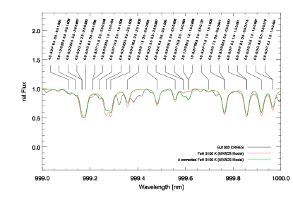
We use the results from the Voigt fit to assign the individual Voigt profiles from the observed lines to the individual theoretical lines. We did this by hand, and define a line as identified if the position of the observed line agrees within Å to the theoretical predicted position. If the offset is larger than Å we identify a line feature if the characteristic shape is similar in the observations and computations (e.g. the line at nm or nm in Fig. 5).
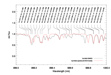
In Fig. 5, and also in the full atlas, we labeled all identified lines with their quantum numbers, i.e. vibrational assignment (), branch (P, Q, R), lower state rotational quantum number , , and in the case of blends, with their contribution to the blend. We did this for the observed wavelength region and the complete plot is available in the online material of this paper. In Fig. 6 we show a histogram of the residuals between the computed line positions and the observed ones. There is no obvious systematic behavior of the scatter with wavelength (see inset in Fig. 6). The scatter follows a normal distribution centered at Å corresponding to km s-1. This mean value is beyond our spectral resolution and in general all residuals smaller than km s Å ) are not significant since they are also smaller than the accuracy of the wavelength calibration. From the investigation of the line positions, we saw that the fraction of lines for which the residuals are smaller than a certain range are distributed as shown in the right inlay of Fig. 6. This plots shows that % of the line features could be identified by their positions which do not deviate by more than Å from the predictions. In the cases where the residuals are larger than Å the uncertainties in the molecular constants which were used to compute the line list are responsible for these deviations.

For our analysis we use only lines with mÅ, which approximately describes a line with % relative flux and a FWHM of Å. We ignore lines with smaller contributions because their intensities are similar to the noise level. However, only lines out of have equivalent widths less than mÅ.
4.2.1 Vibrational bands
From Fig. 2 we expect that the dominant vibrational bands are and from the sequence, and and from the sequence. In Fig. 7 we present a histogram with the number of identified lines for each vibrational band and shows that the expected vibrational bands are present. We also show the number of possible lines from theory with mÅ in the observed wavelength region. This number is based on line by line computation of .
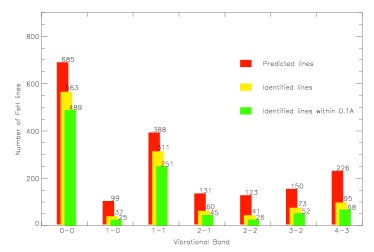
In this histogram the bars in the foreground take into account only the lines identified by their positions.
4.2.2 Coincidence-by-Chance Method
For the lines with residuals smaller than Å we compute the coincidence-by-chance factor from equation 18. In Table 3 the values of , , , and are given for all identified bands. For the and transition, the number of identified lines exceeds the number of coincidences by chance , which is a clear indication that these bands are present in the investigated region. For the other bands the situation is not so clear and we will confirm them with further investigations.
| Band | Wavelength [Å ] | [#/Å ] | () | |
|---|---|---|---|---|
| 360 | 3.73 | 489 (658) | ||
| 52 | 3.74 | 25 (99) | ||
| 208 | 3.71 | 251 (388) | ||
| 68 | 3.76 | 45 (131) | ||
| 65 | 3.81 | 26 (123) | ||
| 79 | 3.78 | 52 (150) | ||
| 119 | 3.75 | 68 (226) |
4.2.3 Cross-Correlation Method
We use cross-correlation techniques to investigate the agreement between the theoretical line list and the observed spectra. As a reference and a test, we cross-correlate a computed spectrum from this theoretical line list, which is broadened by an instrumental profile with a resolving power of , with the original line list (e.g. Fawzy, 1995; Fawzy et al., 1998). To be specific, we vary the theoretical positions with steps of Å in a range of Å and measure the relative intensity, at the different positions, weighted with of the line and integrate over all lines. We then normalize the results with the number of lines in the line list. We do this for all lines in the vibrational bands which are found in the M dwarf spectra (see Fig. 8). If a vibrational band is present, a peak around zero appears above the noise produced by random coincidences with other lines.
We produce three different curves. For the first one, we use all possible lines from the original line list for comparison with the observed stellar spectrum (solid line in Fig. 8). For the second curve we compute a reference curve by cross correlating the original line list with a synthetic spectrum computed from it (dashed line in Fig. 8). This case produces the maximum possible correlation. A third curve is produced using the corrected line list containing only identified lines and we compare it with the observed stellar spectrum (dotted line in Fig. 8).
As expected, for the synthetic spectrum with the theoretical line list (dashed line), all bands show clear peaks above the noise. For the observed spectrum (solid line) and original line list, the and vibrational bands show clear peaks above the noise, which is in agreement with the coincidences by chance values in Table 3. After improving the FeH line list (dotted line), all bands show peaks above the noise similar to the peaks obtained in the reference case from cross-correlating the theoretical line list with the computed spectra. The original theoretical line positions for the , , , , and bands are not accurate enough to show significant peaks in the cross correlation. To confirm our identifications, we also use the line strength in the next section.

4.2.4 Line Intensity Method
We use the method described in Sec.3 to test if the tentatively identified observed lines can be identified with the theoretical ones. We plot against (see equation 23) for the identified vibrational bands, branches, and , using an appropriate estimated error (see Fig. 9).
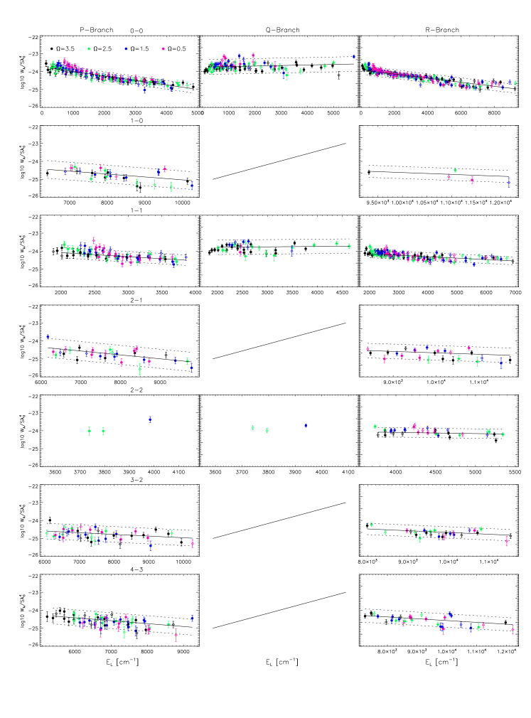
In almost all cases a linear correlation is visible. In some cases where lines with small are present, we see a deviation from the straight line. This deviation is expected due to different heights of formation for the lines. We calculated model plots with synthetic lines, which reproduces this behavior in detail (Fig. 10).
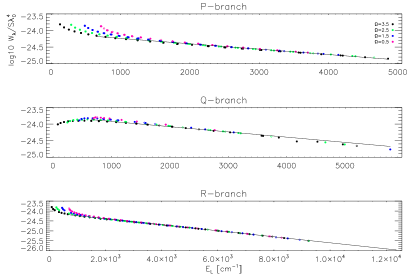
The computations are very similar to the observations, which supports the assumption of different heights of formation. To test this assumption, we computed the contribution function for the lines (Magain, 1986) and use them to determine a weighted mean of the continuum optical depth, . The latter describes a representative atmospheric line formation depth. In Fig. 11, we plotted and against for each branch from the band. These plots show clearly that for the P- and R-lines with low and very high originate in deeper layers than the lines with medium . We also see that the lines with low and high are the ones with small because the Hönl-London factors for P- and R-lines are proportional to and hence the lines become stronger for large , but they also decrease for large due to their increasing s. Hence, there is a maximum in for medium . In the case of Q-branch lines, the situation is different. The Hönl-London factors decrease with increasing and hence the line strength monotonically decreases with . In this case, the lines with low are the lines with the largest and hence these lines are formed in higher layers and the Q-branch shows the opposite behavior to the P- and R-branches in the plot.
We can conclude that in deeper layers, where weak lines are formed, the equivalent width is enhanced by the larger number of molecules that contribute to the absorption (see Fig. 12). The molecule number increases towards deeper layers due to the higher overall density even though the concentration of molecules relative to and decreases. Towards higher temperatures in deeper layers or in hotter stars, the number of molecules would decrease again due to the ionisation of which is then no longer available for the formation of the molecule. In our case, this behaviour results in a deviation from a straight line in Fig. 9
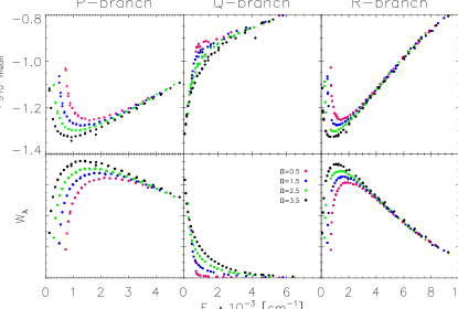

With this knowledge, we can use the line strength to confirm the identification of . In Fig. 9, clearest correlations are found for the and bands which have also the largest number of lines, but also for the P-branch of the and transitions and the R-branch of the transition. The and transitions show also linear correlations but with a larger scatter. This result is a strong indication that all the identified bands are present in the observed spectra. Although the Q-branches of the and bands show no clear linear dependence for large , we expect them to be present and correctly identified, since they show the expected downward trend for small energies. The scatter towards higher energies is much larger than in the other branches and there are only a few measurements. The slope seems to be positive, but we could expect it to be negative if we would have more data points.
We fit the data points linearly for lines with (to avoid the region where the influence of variable number is too strong) and use the difference of the data points from the fit as a measure for the confidence of an identified line. A line is classified as “P” if the difference between and the linear fit is smaller than three times the standard deviation of the scatter around the fit. But we assume that lines with are also present, since they show exactly the expected behavior. It is classified as “Pb” if the deviation is greater than and the data point is above the linear fit and as “R” if it is below. It is classified as “Q” if the line could not be investigated because we only investigated lines with . We give a list of all identified lines with quantum numbers and corrected wavelength in Table 4. This list is explained in more detail in the appendix.
| blend | class | comment | |||||||||||||
| 9900.4846 | 9900.4902 | 0 | 0 | 3.5 | 3.5 | 17.5 | 18.5 | 3 | 470924.44 | 0.8309 | 0.225 | 0.0056 | 1.000 | P | |
| 9901.1049 | 9901.1175 | 0 | 0 | 3.5 | 3.5 | 14.5 | 15.5 | 3 | 462792.47 | 1.0695 | 0.154 | 0.0126 | 1.000 | P | |
| 9901.4704 | 9901.4116 | 0 | 1 | 3.5 | 3.5 | 32.5 | 31.5 | 1 | 133973.65 | 0.3378 | 0.794 | -0.0588 | 1.000 | P | |
| 9903.9631 | 9903.9809 | 0 | 0 | 3.5 | 3.5 | 18.5 | 19.5 | 3 | 472886.88 | 1.1484 | 0.252 | 0.0178 | 0.998 | P | |
| 9904.9843 | 9904.9913 | 0 | 0 | 3.5 | 3.5 | 13.5 | 14.5 | 3 | 458947.25 | 1.4267 | 0.134 | 0.0070 | 1.000 | P | |
| 9905.8556 | 9905.8940 | 0 | 0 | 3.5 | 3.5 | 15.5 | 16.5 | 3 | 466010.13 | 1.1121 | 0.177 | 0.0384 | 0.969 | P | |
| 9905.8556 | 9905.8940 | 3 | 4 | 3.5 | 3.5 | 5.5 | 4.5 | 1 | 93477.74 | 1.1121 | 0.649 | 0.0384 | 0.026 | P | |
4.3 Corrections to the line strengths
If we want to use equation 27 to correct for the differences in line depth, we have to match the stellar parameters as closely as possible. These parameters are basically effective temperature, surface gravity and chemical composition, as well as van der Waals broadening constants, whose influence become significant at these low temperatures. Van der Waals broadening is computed with Unsöld’s hydrogenic approximation, and an enhancement factor is used model the line wings correctly. Since for no enhancement factor is reported, we need to determine one. For M-type stars, an assumed surface gravity of is standard and the chemical composition is usually assumed as solar. To match the strong Ti lines in the – Å region as well as the lines, we have to increase the iron abundance from to the Grevesse & Anders (1989) value of . We use this scaling as a parameter and do not claim this to be the actual iron abundance of GJ1002. The free parameters for GJ1002 are now , van der Waals broadening enhancement factor (which we call from now on ), and the instrumental resolving power, which we use as a fitting parameter to account for possible additional rotational broadening. These three parameters are strongly correlated. We create maps to determine the most likely combination that matches the observed spectra best.
4.3.1 maps
For the comparison between observation and computation we chose a region where the original line list fits best, the lines are strongest and hence the influence of van der Waals broadening is largest. We selected the first Å from the band head at Å . For the computations we use our new line list with corrected positions and include also the identified atomic lines. To create the maps for the three combinations of parameters, we search for the minimum for each parameter (light cross in left plots in Fig. 13) and use this value to construct the map for the other two parameters. The maps (right hand side in Fig. 13) yield a consistent picture of the parameter combinations for the spectra of GJ1002.
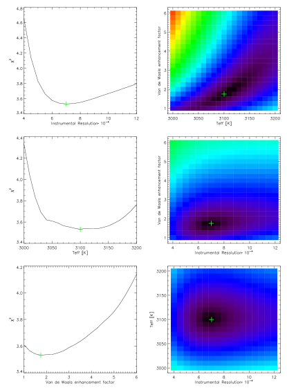
The most likely parameters for effective temperature, resolving power, and are K, and , respectively. It is obvious, however, that the curves show regions with broad minima which would allow for variations in the derived parameters.
Since the observed spectra are supposed to have a resolving power of , the difference from our determined resolving power stems probably from rotation, which is measured to be lower then km s-1, but not necessarily zero. The difference in resolving power results in km s-1 at a wavelength of Å .
An independent constraint for the instrumental resolving power and effective temperature is given by the Ti lines, which are strong and distributed over a wide wavelength range in the spectra. The computation of these lines with the parameters and broadening constants given by VALD fits the observations within % for the line depth. This gives us confidence that the decreasing line depth of the lines with increasing wavelength is a real feature and not due to normalisation effects.
4.3.2 Einstein A values
In order to correct for the Einstein A values we use computed spectra which have already corrected line positions. We iteratively adjust the Einstein A values because for saturated lines the first scaling is not sufficient. The scaling factors for each line are listed in the Table 4 and an example for the corrected computed spectra is shown in Fig. 14. In order to estimate an error, we assume an accuracy of for the observed line depth, which results in an error of for the scaling factors. If we furthermore assume that the line depth is modified by an unknown blended feature by, e.g., an error of follows. The accuracy of the Einstein A scaling is also influenced by the van der Waals enhancement factor . A change of gives a mean difference of in the scaling constants, but can be up to for individual lines, due to the logarithmic ratio of the intensities (see e.g. equation 27).
We obtain a good fit to the data with the scaled Einstein A values even for some lines calculated to be very weak. However this results in some cases in unrealistic values, and we assume that these weak lines are blended with unknown components. The scaling of line blends is a difficult problem because it results in equal scaling factors for lines with completely different quantum numbers. To avoid this problem one could determine scaling factors for each branch, but we chose the simpler scheme of scaling each line.
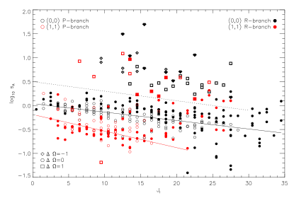
We use equation 27 and plot for the Einstein A values against to search for a possible rotational dependence (Fig. 15). We plot only scaling factors for the and bands, since these are the bands with the largest number of lines and we use only lines which contribute more than % to a blended line feature in order to avoid contributions from incorrectly scaled lines.
We find two groups of scaling factors. One group describes a strong enhancement of the line depths (‘positive’ scaling factors) and the other only a small enhancement for low and a reduction towards lines with large (‘negative’ scaling factors). We divide these two groups by a dashed line in Fig. 15. For the transitions of the and bands we include linear fits to the data in Fig. 15 to indicate the slope.
The group of positive scaling factors is strongly dominated by transitions (diamonds and rectangles), while the group of negative scaling factors consists of only transitions (circles). The latter scaling factors for and bands (black and red circles, open for P-branches and filled for R-branches) show an almost linear behaviour with and become stronger towards larger . The positive scaling factors show also two linear groups, which originate from the band (red rectangles) and from the band (black diamonds and rectangles). These scaling factors describe a strong enhancement of the lines for small and become smaller towards large . All groups of scaling factors have a similar negative slope, and are only shifted by a constant factor to higher or lower scaling factors.
The distribution of other bands and lines which contribute less than % to a blended feature gives only a larger scatter to the data points, but does not change the basic trend of the scaling factors. We conclude that the dependence in the scaling factors likely indicates shortcomings in the calculated Hönl-London factors. In particular, satellite branches with are much stronger than expected for Hund’s case (a). In other words, the two electronic states are heavily mixed with other electronic states and the simple Hund’s case (a) behaviour anticipated for isolated electronic states with relatively large spin-orbit splittings is not found.
4.4 Rotational temperatures
A rotational temperature can be obtained from the slope of the linear fit in the diagram described in the above section. can be calculated from
| (29) |
For the fit to the data, we use only lines with in order to avoid the significant influence from varying absorber number, and neglect lines with line depth greater than to avoid saturation effects.
Due to the large errors (derived from the uncertainty of the slope of the linear fit in Fig. 9), we consider only rotational temperatures with moderately small one sigma errors (see Fig. 16).
We find systematically lower temperatures for the P-branches in comparison to the R-branches which is consistent with different heights of formation for most of the lines in a branch as seen in Fig. 11.
If we compute the weighted mean of the rotational temperatures (grey solid line in Fig. 16) with the -error (grey dashed-line in Fig. 16), we obtain K . This is in the middle of the expected temperature range for this spectral type ( K– K, dashed-dotted lines in Fig. 16) and is close to our estimated value of K. The main contribution to stems from the P- and R-branches of the transition due to their small uncertainties. The weighted mean of the P- and R-branches are K and K, respectively.
We want to point out that even for a single branch in a band, the obtained temperature is an average over the individual excitation temperatures for each line. The resulting temperature depends crucially on the selection of the lines that are used. If one uses lines with similar equivalent width and lower level energy, then one could obtain temperatures for certain regions in the atmosphere. For this method, however, a large number of lines is required, because otherwise the uncertainties become too large.
We conclude that in order to use the method of rotational temperatures, a large number of well measured lines are required to minimize the error in the slope. Finally, the rotational temperature can only be expected to match the effective temperature if the lines form in a region around optical depth unity.

5 Summary and conclusion
We investigated the z-band region of the M5.5 dwarf GJ1002 with high-resolution CRIRES spectra. This is the region where the vibrational band of is present (‘Wing-Ford band’). We were able to identify the , , , , , , and bands. For confirmation of the band assignment, we used the method of coincidence, cross-correlation techniques, and the line intensities.
For the identified lines, we applied empirical corrections to the theoretical line positions. The deviations between observed and computed positions are Gaussian distributed around zero. In the case of small deviations ( Å ), this could be due to uncertainties in the wavelength calibration of the observed spectra and in other cases due to uncertainties in the molecular constants which were used to generate the line list. Note that these empirical wavelength adjustments reproduce the observed stellar spectrum, but the quantum number assignments are by no means assured.
The method of coincidence confirms the presence of the and bands, but for the other bands we needed cross-correlation techniques to show their presence. Again the and bands show clear peaks in the cross-correlation function even with an uncorrected line list, but for the other bands it was necessary to use corrections to the line list in order to confirm them. We also used line intensity information by plotting the ratio against which shows a linear behaviour if the band is present in the spectra. With this method we could confirm the presence of all the other bands although not uniquely for the Q-branches.
From the slope of the line in the plots, it was possible to derive excitation temperatures for rotational transitions, which could be identified with the effective temperature of the star if the lines are formed in the photosphere. We showed that this method is very uncertain since the error in the slope is high. The derived temperatures for the individual vibrational transitions range from K to K for GJ1002, but the weighted mean K is very close to the expected temperature of an M 5.5 dwarf. However, the large error bars and differences between P- and R-branch temperatures suggests that this agreement may be more of a coincidence than a physical result.
Finally we corrected the line strength in the line list by scaling the Einstein A values, as some of these lines show large discrepancies compared to the observations. For this purpose it was necessary to derive the instrumental broadening (which included the rotational broadening), effective temperature, and an enhancement factor for the van der Waals broadening constants. The instrumental resolving power was derived to , which is equivalent to a rotational broadening with km s-1. We also derived an effective temperature of K, and a van der Waals enhancement constant of . The scaling factors of the Einstein A values show an almost linear dependence on , which indicates that there is likely a problem in the calculation of the Hönl-London factors.
With the improved identification of lines, it is now possible to characterize the lines in the z-band region (e.g. magnetically sensitive and insensitive lines, temperature sensitivities of individual lines). Our improved line list will aid in the identification and simulation of lines in spectra of cool stars.
Appendix
Explanation of the FeH Table
The Table 4 contains the observed wavelength which are obtained with the Voigt fit and the theoretical wavelength from the list of Dulick et al. (2003). The wavelengths are in vacuum. We give also the quantum numbers of the lines and the Einstein A values with their scaling factors . The lower level energy is given in eV. The difference in position is also printed in the table. If the line is a blended line, then its contribution to the blend is given as the fraction normalized to one. If the line is not blended its blend value is one. We give then the classification of the line, as defined in section 3.3. We add a comment if the line is blended by an atomic feature, or if the classification of the line did not agree with the scaling factor of the Einstein A values.
Explanation of the FeH Atlas
We plotted the whole spectrum in bins of nm from nm to nm. Shown are the observed spectrum of GJ1002 (black), the computed spectrum with corrected positions (red), the computed spectrum with corrected positions and scaled Einstein A values (green). We also labeled all lines with mÅ with quantum number for the vibrational transition, the branch, the lower , the upper and lower , and in the last position, their blend fraction. The blend fraction is unity if a line is not blended. We also labeled the position of atomic lines with the element name below the spectrum.
Acknowledgements.
SW would like to acknowledge the support from the DFG Research Training Group GrK - 1351 “Extrasolar Planets and their host stars”.AR acknowledges research funding from the DFG under an Emmy Noether Fellowship (RE 1664/4- 1).
AS acknowledges financial support DFG under grant RE 1664/4- 1 and from NSF under grant AST07-08074.
Some support to PFB was provided by the NASA laboratory astrophysics program.
We thank P. Hauschildt and D. Shulyak for useful discussions.
References
- Afram et al. (2007) Afram, N., Berdyugina, S. V., Fluri, D. M., et al. 2007, A&A, 473, L1
- Afram et al. (2008) Afram, N., Berdyugina, S. V., Fluri, D. M., Solanki, S. K., & Lagg, A. 2008, A&A, 482, 387
- Baschek et al. (1966) Baschek, B., Holweger, H., & Traving, G. 1966, Astronomische Abhandlung der Hamburger Sternwarte, 8, 26
- Bernath (2005) Bernath, P. 2005, Spectra of Atoms and Molecules (Oxford Oxfordshire: Oxford University Press)
- Cushing et al. (2003) Cushing, M. C., Rayner, J. T., Davis, S. P., & Vacca, W. D. 2003, ApJ, 582, 1066
- Dulick et al. (2003) Dulick, M., Bauschlicher, Jr., C. W., Burrows, A., et al. 2003, APJ, 594, 651
- Fawzy (1995) Fawzy, D. E. 1995, Master’s thesis, M. Sci.-Thesis, Cairo University (1995)
- Fawzy et al. (1998) Fawzy, D. E., Youssef, N. H., & Engvold, O. 1998, A&AS, 129, 435
- Gray (2008) Gray, D. F. 2008, The Observation and Analysis of Stellar Photospheres (The Observation and Analysis of Stellar Photospheres, by D.F. Gray. Cambridge: Cambridge University Press, 2008.)
- Grevesse & Anders (1989) Grevesse, N. & Anders, E. 1989, in American Institute of Physics Conference Series, Vol. 183, Cosmic Abundances of Matter, ed. C. J. Waddington, 1–8
- Grevesse et al. (2007) Grevesse, N., Asplund, M., & Sauval, A. J. 2007, Space Science Reviews, 130, 105
- Gustafsson et al. (2008) Gustafsson, B., Edvardsson, B., Eriksson, K., et al. 2008, A&A, 486, 951
- Hargreaves et al. (2010) Hargreaves, R., Hinkle, K. H., Bauschlicher, C. W., et al. 2010, AJ
- Kochukhov (2007) Kochukhov, O. P. 2007, in Physics of Magnetic Stars, 109–118
- Kupka et al. (2000) Kupka, F. G., Ryabchikova, T. A., Piskunov, N. E., Stempels, H. C., & Weiss, W. W. 2000, Baltic Astronomy, 9, 590
- Magain (1986) Magain, P. 1986, A&A, 163, 135
- Nordh et al. (1977) Nordh, H. L., Lindgren, B., & Wing, R. F. 1977, A&A, 56, 1
- Phillips et al. (1987) Phillips, J. G., Davis, S. P., Lindgren, B., & Balfour, W. J. 1987, ApJS, 65, 721
- Reiners & Basri (2006) Reiners, A. & Basri, G. 2006, ApJ, 644, 497
- Reiners & Basri (2007) Reiners, A. & Basri, G. 2007, ApJ, 656, 1121
- Russell & Bowen (1929) Russell, H. N. & Bowen, I. S. 1929, ApJ, 69, 196
- Sauval & Tatum (1984) Sauval, A. J. & Tatum, J. B. 1984, ApJS, 56, 193
- Schadee (1964) Schadee, A. 1964, Bull. Astron. Inst. Netherlands, 17, 311
- Schiavon et al. (1997) Schiavon, R. P., Barbuy, B., & Singh, P. D. 1997, ApJ, 484, 499
- Schweitzer et al. (1996) Schweitzer, A., Hauschildt, P. H., Allard, F., & Basri, G. 1996, MNRAS, 283, 821
- Wallace et al. (1998) Wallace, L., Hinkle, K., & Livingston, W. 1998, An atlas of the spectrum of the solar photosphere from 13,500 to 28,000 cm-1 (3570 to 7405 A), ed. Wallace, L., Hinkle, K., & Livingston, W.
- Wallace et al. (1999) Wallace, L., Livingston, W. C., Bernath, P. F., & Ram, R. S. 1999, An atlas of the sunspot umbral spectrum in the red and infrared from 8900 to 15,050 cm(-1) (6642 to 11,230 [angstroms]), revised, ed. Wallace, L., Livingston, W. C., Bernath, P. F., & Ram, R. S.
- Wende et al. (2009) Wende, S., Reiners, A., & Ludwig, H. 2009, A&A, 508, 1429
- Wing (1972) Wing, R. F. 1972, in Les Spectres des Astres dans l’Infrarouge et les Microondes, 123–140
- Wing & Ford (1969) Wing, R. F. & Ford, W. K. J. 1969, PASP, 81, 527
- Wöhl (1970) Wöhl, H. 1970, Sol. Phys., 15, 342