Spin interactions in a quantum dot containing a magnetic impurity

Abstract

The electron and hole states in a CdTe quantum dot containing a single magnetic impurity in an external magnetic field are investigated, using the multiband approximation which includes the heavy hole-light hole coupling effects. The electron-hole spin interactions and s,p-d interactions between the electron, the hole and the magnetic impurity are also included. The exciton energy levels and optical transitions are evaluated using the exact diagonalization scheme. A novel mechanism is proposed here to manipulate impurity-spin in the quantum dot which allows us to drive selectively the spin of the magnetic atom into each of its six possible orientations.

1 Introduction

Quantum dots (QDs), the nanoscale zero-dimensional systems with discrete energy levels, much like in atoms (and hence the popular name, artificial atoms [1]) have one great advantage that the shape and the number of electrons and holes in those systems can be controlled externally and as a result, these systems have been the subject of intense research in recent years. In the QDs it is therefore possible to localize single spin in an area of a few nanometers. Conservation of the angular momentum in the QD allows for both spin sensitive detection and injection. By coupling these techniques with ultrafast optical pulses, it is possible to stroboscopically measure the spin dynamics in a QD. Thus QDs are particularly promising as components of futuristic devices for quantum information processing and for coherent spin transport [2].

Detection and control of single magnetic atoms in QDs represent the fundamental scaling limit for the magnetic information storage. The strong and electronically controllable spin-spin interactions that exists in magnetic semiconductors offer an ideal laboratory for exploring the single magnetic spin readout and control. Magnetic ions placed within a lattice can exhibit relatively long spin lifetimes [3]. Exploration of single magnetic spins in semiconductor QDs was pioneered in (II,Mn)-VI systems where the magnetic atoms are isoelectronic Mn²⁺ ions with spin 5/2 (see e.g. [4, 5, 6]). A different situation arises in (III,Mn)-V magnetic semiconductors, where the Mn²⁺ ions contribute to the acceptor states within the band gap causing the magnetic ions to behave as optical spin centers [7]. Experiments have clearly illustrated the effect of magnetic ions on exciton optical spectrum in the QDs [8]. Theoretically, the effect of spin-exciton interactions on the optical spectrum of a quantum dot with a magnetic impurity is considered in [9]. But due to approximations used in [9], the results are limited only to the case of zero or low magnetic fields. Recently Gall et. al. [10] presented a new way to optically probe the spin of a single magnetic impurity in the QD. They demonstrated that optical excitation of an individual Mn-doped QD with circularly polarized photons can be used to prepare nonequilibrium distribution of the Mn spin, even in the absence of an applied magnetic field. Reiter et. al. [11] have presented a technique for an all-optical switching of the spin state of a magnetic atom in a QD on a picosececond time scale. They have shown that the spin state of a single Mn atom in a QD can be selectively controlled by manipulating the exciton states with ultrafast laser pulses. All six possible spin states can be reached. The switching process can be optimized by applying a magnetic field.

In this paper we report on our theoretical studies involving electron and hole states in a CdTe quantum dot containing a single magnetic impurity in an external magnetic field. Here we show that the s,p-d spin interaction brings about level anticrossings between the dark and bright exciton states. We explain the physics behind these anticrossings. Our results are in good agreement with the experimental observations [8]. We also propose a new magneto-optical mechanism for manipulation of the magnetic impurity spin, by using the laser pulses and by varying the strength of the magnetic field.

2 Theory

In our investigation of the electron and hole states in a cylindrical CdTe quantum dot with a single magnetic impurity, subjected to a perpendicular magnetic field, we choose the lateral confinement potential of the dot as parabolic with the corresponding frequencies $\omega_{0}^{e}$ and $\omega_{0}^{h}$ for electron and hole respectively. This choice can be justified from the energies of the far-infrared absorption on such dots, which shows only a weak dependence on the electron occupation [12, 13]. We also take into account the confinement potential in the growth direction as a rectangular well of width $L$. We assume that the size of the dot is smaller than the bulk exciton Bohr radius and neglect the long-range electron-hole Coulomb interaction [14, 15]. The Hamiltonian of the system can then be written as

$${\cal H}={\cal H}_{e}+{\cal H}_{h}+{\cal H}_{s-d}+{\cal H}_{p-d}+{\cal H}_{eh},$$ (1)

where ${\cal H}_{s-d}=-J_{e}\delta({\bf r}_{e}-{\bf r}_{Mn})\boldsymbol{\sigma}{\bf S}$ and ${\cal H}_{p-d}=-J_{h}\delta({\bf r}_{h}-{\bf r}_{Mn}){\bf j}{\bf S}$ describe the electron-Mn and hole-Mn spin-spin exchange interaction with strengths $J_{e}$ and $J_{h}$ respectively. ${\cal H}_{eh}=-J_{eh}\delta({\bf r}_{e}-{\bf r}_{h})\boldsymbol{\sigma}\bf{j}$ is the electron-hole spin interaction Hamiltonian [14].

The electron Hamiltonian is

$${\cal H}_{e}=-{\frac{1}{2m_{e}}}\left({\bf p}-{\frac{e}{c}}{\bf A}\right)^{2}+V_{conf}^{e}(\rho,z)+\frac{1}{2}g_{e}\mu_{B}B\sigma_{z},$$ (2)

where ${\bf A}=B/2(-y,x,0)$ is the vector potential of magnetic field in the symmetric gauge and the last term is the electron Zeeman energy. The eigenfunctions of ${\cal H}_{e}$ can be written as

$$\psi_{nls\sigma}^{e}(\rho,\theta,z)=f_{nl}^{e}(\rho)e^{il\theta}g_{s}(z)\chi_{\sigma},$$ (3)

where $\chi_{\sigma}$ are the electron spin functions,

$$g_{s}(z)=\sqrt{\frac{2}{L}}\sin\left[{\frac{s\pi}{L}}\left(z+{\frac{L}{2}}\right)\right]\qquad s=1,2,3,\ldots$$

and the in plane functions are Fock-Darwin orbitals [1]

$$f_{nl}(\rho)=C_{nl}e^{-\frac{\rho^{2}}{2a_{e}^{2}}}\left(\frac{i\rho}{a_{e}}\right)^{|l|}L_{n}^{|l|}\left(\frac{\rho^{2}}{a_{e}^{2}}\right)$$ (4)

$$C_{nl}=\frac{1}{a}\left[\frac{n!}{\pi(n+|l|)!}\right]^{\frac{1}{2}},\quad n=0,1,2,\ldots,\quad l=0,\pm 1,\pm 2,\ldots$$

The single-electron energy is given by

$$E_{nls\sigma}=2\hbar\omega_{e}\left(n-l\frac{\omega_{c}^{e}}{4\omega_{e}}+\frac{|l|+1}{2}\right)+\frac{\hbar^{2}\pi^{2}s^{2}}{2m_{e}L^{2}}+g_{e}\mu_{B}B\sigma,$$

where $\omega_{c}^{e}=eB/m_{e}c$ is the cyclotron frequency, $\omega_{e}=\sqrt{(\omega_{o}^{e})^{2}+0.25(\omega_{c}^{e})^{2}}$ and $a_{e}=\sqrt{\hbar/m_{e}\omega_{e}}$.

Taking into account only the $\Gamma_{8}$ states which correspond to the states with the hole spin $j=3/2$ and include the heavy hole-light hole coupling effects, we can construct the single-hole Hamiltonian in the dot as

$${\cal H}_{h}={\cal H}_{L}+V_{conf}^{h}(\rho,z)-2\kappa\mu_{B}Bj_{z}.$$ (5)

Here ${\cal H}_{L}$ is the Luttinger hamiltonian in axial representation obtained with the four-band k$\cdot$p theory [16, 17]

$${\cal H}_{L}=\frac{1}{2m_{0}}\left(\begin{array}[]{cccc}{\cal H}_{h}&R&S&0\\ R^{*}&{\cal H}_{l}&0&S\\ S^{*}&0&{\cal H}_{l}&-R\\ 0&S^{*}&-R^{*}&{\cal H}_{h}\end{array}\right),$$ (6)

where

$${\cal H}_{h} = (\gamma_{1}+\gamma_{2})(\Pi_{x}^{2}+\Pi_{y}^{2})+(\gamma_{1}-2\gamma_{2})\Pi_{z}^{2},$$

$${\cal H}_{l} = (\gamma_{1}-\gamma_{2})(\Pi_{x}^{2}+\Pi_{y}^{2})+(\gamma_{1}+2\gamma_{2})\Pi_{z}^{2},$$

$R=2\sqrt{3}\gamma_{3}{\rm i}\Pi_{-}\Pi_{z},\quad S=\sqrt{3}\gamma\Pi_{-}^{2},\quad\gamma=\frac{1}{2}(\gamma_{2}+\gamma_{3}),$ and ${\bf\Pi}={\bf p}-\frac{e}{c}{\bf A},\quad\Pi_{\pm}=\Pi_{x}\pm{\rm i}\Pi_{y}.$ $\gamma_{1},\gamma_{2}$, $\gamma_{3}$ and $\kappa$ are the Luttinger parameters and $m_{0}$ is the free electron mass.

The Hamiltonian (5) is rotationally invariant. Therefore it will be useful to introduce the total momentum ${\bf F}={\bf j}+{\bf l}$, where ${\bf j}$ is the angular momentum of the band edge Bloch function, and ${\bf l}$ is the envelop angular momentum. Since the projection of the total momentum $F_{z}$ is a constant of motion, we can find simultaneous eigenstates for (5) and $F_{z}$ [18].

For the given value of $F_{z}$ it is logical to seek the eigenfunctions of Hamiltonian (5) as an expansion [17, 19]

$$\Psi_{F_{z}}(\rho,\theta,z)=\sum_{n,s,j_{z}}C_{F_{z}}(n,s,j_{z})f_{n,F_{z}-j_{z}}^{h}(\rho)e^{i(F_{z}-j_{z})\theta}g_{s}(z)\chi_{j_{z}},$$ (7)

where $\chi_{j_{z}}$ are hole spin functions and $f_{nl}^{h}(\rho)$ are the Fock-Darwin orbitals for hole with $a_{h}=\sqrt{\hbar(\gamma_{1}+\gamma_{2})/m_{0}\omega_{h}}$, $\omega_{h}=\sqrt{(\omega_{o}^{h})^{2}+0.25(\omega_{c}^{h})^{2}}$ and $\omega_{c}^{h}=eB(\gamma_{1}+\gamma_{2})/m_{0}c$. The matrix elements of the Hamiltonian (5) can then be evaluated analytically. All single hole energy levels and expansion coefficients are evaluated numerically using the exact diagonalization scheme [19]. Calculations are carried out for the CdTe quantum dot with sizes $a_{e}=a_{h}=37$ Å, $L=25$Å and with following parameters: $E_{g}=1.59$ eV, $m_{e}=0.096m_{0}$, $g_{e}=-1.5$ $\gamma_{1}=5.29$, $\gamma_{2}=1.8$, $\gamma_{3}=2.46$, $\kappa=0.7$ [20].

To include spin-spin interactions, we can construct the wave function of the electron, hole and the magnetic impurity as an expansion of direct products of the lowest state wave functions (3), (7) and eigenfunctions for the magnetic impurity.

$$\Psi_{J_{z}}=\sum_{\sigma}\sum_{F_{z}}\sum_{S_{z}}C(\sigma,F_{z},S_{z})\psi_{0,0,1,\sigma}^{e}\times\psi_{F_{z}}^{h}\times|S_{z}\rangle.$$ (8)

Here $\sigma=\pm 1/2$, $S_{z}=\pm 1/2,\pm 3/2,\pm 5/2$ and $F_{z}=\pm 1/2,\pm 3/2,\pm 5/2\ldots$ and $J_{z}$ is the projection of the total momentum ${\bf J}={\bf\sigma}+{\bf F}+{\bf S}$. Using the components of this expansion as the new basis functions, we can calculate the corresponding matrix elements for the electron-hole, the electron-impurity and the hole-impurity interactions. For the electron-hole interaction we have

$$M_{eh}=-2\pi J_{eh}\delta_{S_{z},S_{z}^{\prime}}\sum_{nsj_{z}}\sum_{n^{\prime}s^{\prime}j_{z}^{\prime}}C_{F_{z}}(n,s,j_{z})C_{F_{z}^{\prime}}(n^{\prime},s^{\prime},j_{z}^{\prime})\delta_{F_{z}-j_{z},F_{z}^{\prime}-j_{z}^{\prime}}\times$$

$$\int_{0}^{\infty}\left|f_{00}^{e}(\rho)\right|^{2}\left(f_{n,F_{z}-j_{z}}^{h}(\rho)\right)^{*}f_{n^{\prime},F_{z}^{\prime}-j_{z}^{\prime}}^{h}(\rho)\rho d\rho\times$$

$$\int_{-L/2}^{L/2}\left(g_{1}^{e}(z)\right)^{2}g_{s}^{h}(z)g_{s^{\prime}}^{h}(z)dz\times\left\langle\sigma,j_{z}|\boldsymbol{\sigma}{\bf j}|\sigma^{\prime},j_{z}^{\prime}\right\rangle,$$ (9)

where $\boldsymbol{\sigma}$ is the Pauli spin operator and $\bf{j}$ is the hole spin operator with following components

$$j_{x}=\left(\begin{array}[]{cccc}0&\frac{{\rm i}\sqrt{3}}{2}&0&0\\ -\frac{{\rm i}\sqrt{3}}{2}&0&{\rm i}&0\\ 0&-{\rm i}&0&\frac{{\rm i}\sqrt{3}}{2}\\ 0&0&-\frac{{\rm i}\sqrt{3}}{2}&0\\ \end{array}\right),\qquad j_{y}=\left(\begin{array}[]{cccc}0&\frac{\sqrt{3}}{2}&0&0\\ \frac{\sqrt{3}}{2}&0&1&0\\ 0&1&0&\frac{\sqrt{3}}{2}\\ 0&0&\frac{\sqrt{3}}{2}&0\\ \end{array}\right),$$

$$j_{z}=\left(\begin{array}[]{cccc}\frac{3}{2}&0&0&0\\ 0&\frac{1}{2}&0&0\\ 0&0&-\frac{1}{2}&0\\ 0&0&0&-\frac{3}{2}\\ \end{array}\right).$$

For the case of electron-impurity interaction we get

$$M_{s-d}=-\frac{J_{e}}{4\pi}\delta_{j_{z},j_{z}^{\prime}}\left|f_{00}^{e}(\rho_{i})\right|^{2}(g_{1}^{e}(z_{i}))^{2}\left\langle\sigma_{z},S_{z}|\boldsymbol{\sigma}{\bf{S}}|\sigma_{z}^{\prime},S_{z}^{\prime}\right\rangle,$$ (12)

where $\rho_{i}$ and $z_{i}$ are the impurity coordinates. Finally for the case of hole-impurity interaction we get

$$M_{p-d}=-\frac{J_{h}}{2\pi}\delta_{\sigma,\sigma^{\prime}}\sum_{n,s,j_{z}}\sum_{n^{\prime}s^{\prime}j_{z}^{\prime}}C_{F_{z}}(n,s,j_{z})C_{F_{z}^{\prime}}(n^{\prime},s^{\prime},j_{z}^{\prime})\times$$

$$\left(f_{n,F_{z}-j_{z}}^{h}(\rho_{i})\right)^{*}f_{n^{\prime},F_{z}^{\prime}-j_{z}^{\prime}}^{h}(\rho_{i})g_{s}^{h}(z_{i})g_{s^{\prime}}^{h}(z_{i})\left\langle j_{z},S_{z}|{\bf{j}}{\bf{S}}|j_{z}^{\prime},S_{z}^{\prime}\right\rangle.$$ (13)

In order to calculate spin matrix elements in (12, 2) we need to introduce the raising and lowering operators $\bf{S_{+}}$ and $\bf{S_{-}}$.

$${\bf{S_{+}}}|S_{z}\rangle=\sqrt{S(S+1)-S_{z}(S_{z}+1)}|S_{z}+1\rangle,$$

$${\bf{S_{-}}}|S_{z}\rangle=\sqrt{S(S+1)-S_{z}(S_{z}-1)}|S_{z}-1\rangle.$$ (14)

When the magnetic impurity is located at the center of the dot, we have non vanishing matrix elements for the hole-impurity interaction only for hole states with $F_{z}=\pm 3/2$ and $\pm 1/2$. Therefore the number of basis states for that case is 48. Since the hole ground state and the first few low-lying states are described by $F_{z}=\pm 3/2$ and $\pm 1/2$, we can use the same 48 basis states also for the case of off-center impurity. The problem was solved numerically using the exact diagonalization scheme and with interaction parameters $J_{e}=15$ meV nm³, $J_{h}=-60$ meV nm³ [8, 11].

3 Discussion

In the absence of a magnetic atom and without the electron-hole spin interaction, the hole ground state is at $F_{z}=\pm 3/2$ and the ground state of the electron-hole pair will be four-fold degenerate with values of total momentum $J_{z}=\pm 1$ and $\pm 2$. The magnetic field lifts that degeneracy due to the Zeeman splitting and as a result two bright ($J_{z}=\pm 1$) and two dark ($J_{z}=\pm 2$) exciton states appear. The electron-hole exchange interaction in turn gives rise to a further splitting between the bright and dark exciton states and removes the degeneracy between them at zero magnetic field.

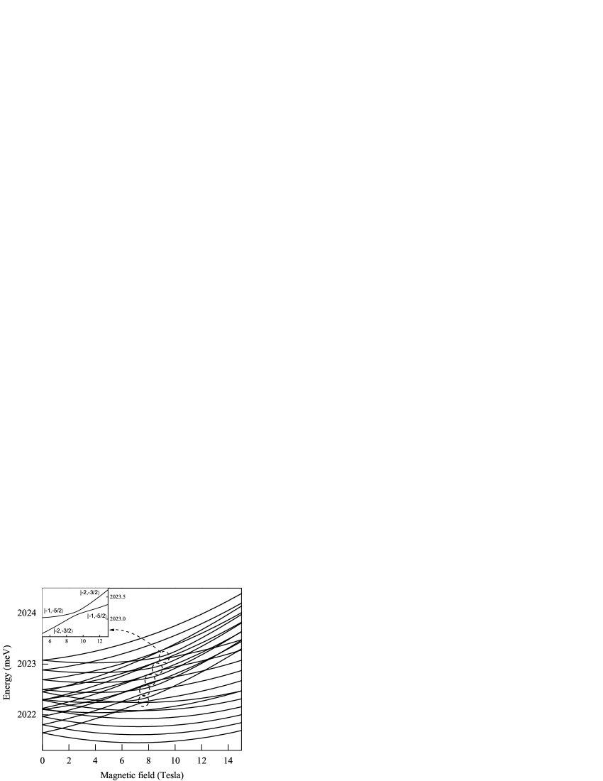
Figure 1: Magnetic field dependence of the electron and hole total energy levels taking into account the sp-d interaction with a magnetic impurity located at the center of the dot. The detailed picture of one of the anticrossings due to spin interaction is presented as inset.

The sp-d exchange interaction between the electron (hole) and the magnetic impurity will split each of these four exciton energy levels to six. As a result, there are 24 separate energy levels. In figure 1, we show the electron-hole energy levels as a function of the magnetic field with the magnetic impurity at the center of the dot. Each state can be presented as a linear superposition of the 48 basis functions defined above. For a given value of the magnetic field, each state can be labeled by the most important component of the basis states. As an example, for the ground state the most important component is $\sigma=1/2$, $F_{z}=3/2$ and $S_{z}=-5/2$ for all values of the magnetic field. So we can label it $|1/2,3/2,-5/2\rangle$ or $|2,-5/2\rangle$. With an increase of the magnetic field we see many level crossings and anticrossings. The most interesting ones are the five anticrossing points, marked by circles in the figure. The reason for these anticrossings is the sp-d interaction between the dark and bright states with same total momentum. For example, the bright exciton state $|-1,-5/2\rangle$ will couple to the dark state $|-2,-3/2\rangle$. As a result, there will be an anticrossing at a magnetic field of 9 Tesla, which is presented as inset of figure 1. The other four anticrossings are due to coupling of the states $|-1,-3/2\rangle$ and $|-2,-1/2\rangle$, $|-1,-1/2\rangle$ and $|-2,1/2\rangle$, $|-1,1/2\rangle$ and $|-2,3/2\rangle$, $|-1,3/2\rangle$ and $|-2,5/2\rangle$. The bright state with the most important component $|-1,5/2\rangle$ and the dark state with $|-2,-5/2\rangle$ have no anticrossings.

Figure 2: Magnetic field dependence of the electron and hole total energy levels taking into account the sp-d interaction with an off-center magnetic impurity. (a) Impurity shifted from the center in grough direction ($\rho_{i}=0$, $z_{i}=2$nm). (b) Impurity shifted from the center in plane direction ($\rho_{i}=3$nm, $z_{i}=0$)

The two energy states in the inset of figure 1 are superpositions of $|-1,-5/2\rangle$ and $|-2,-3/2\rangle$. At low magnetic fields the main component of the higher level is $|-1,-5/2\rangle$ and the weight of $|-2,-3/2\rangle$ is much smaller. Near the anticrossing point the weights of both components are equal, and for high magnetic fields the main component is $|-2,-3/2\rangle$. The opposite picture can be seen for the lower level. This change of the most important component with an increase of the magnetic field will manifest itself in the optical spectrum of the system, which we discuss below.

In Figure 2 the electron-hole energy levels as a function of magnetic field are presented for the case of an off-center impurity. In (a), the impurity is shifted from the center of the dot in growth direction by 2 nm, and in (b) impurity is shifted in the plane by 3 nm. In both cases, the energy splitting due to the s,p-d spin interactions become smaller. This is because the strength of short range spin interaction depends on the probability to find the electron (the hole) at the point of the impurity. Since the ground state electron (hole) is mostly located in the central part of the dot, if we move the impurity out of the central part, all the effects described above will become weaker.

In order to calculate the optical transition probabilities, let us note that the initial state of the system is that of the magnetic impurity spin with the valence band states fully occupied and the conduction band states empty. Let us also assume that the impurity states are pure states $|i\rangle=|S_{z}\rangle$. Recently, there were several experimental reports where quantum dots with a single magnetic impurity in a pure spin state were prepared even in a zero magnetic field [11, 10]. The final states are the eigenstates of the Hamiltonian (1) presented in (8) $|f\rangle=|\Psi_{J_{z}}\rangle$. In the electric dipole approximation the relative oscillator strengths for all possible optical transitions are proportional to

$$P(m)\sim\left|\langle\Psi_{J_{z}}|m,S_{z}\rangle\right|^{2}.$$ (15)

Here the values of $m=1,0,-1$ characterize the polarization of the light as $\sigma^{+}$, $\pi$ and $\sigma^{-}$ respectively [4]. It should also be mentioned that the impurity spin state remains unchanged during the optical transitions.

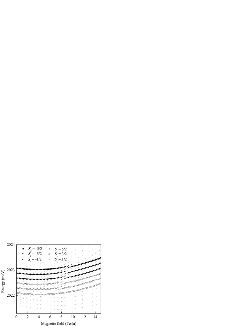
Figure 3: Optical transition energies versus the magnetic field. The shape of the points indicates the impurity spin of initial state, while the size of the points illustrate the probability of the transition.

In figure 3 all possible optical transition energies of the system are presented as a function of the magnetic field for $\sigma^{-}$ polarization of the light and for six different initial states of the magnetic impurity. The shapes of the points indicate the initial spin of the impurity and the sizes indicate the probability of transition. In the case of the initial state with $S_{z}=5/2$ the optical transition is possible only to the final states which have projection to bright exciton state $|-1,5/2\rangle$ (white squares in figure 3). We only have one state with the most important component $|-1,5/2\rangle$ for all values of the magnetic field. We thus see only one line with high transition probability. For the initial state $S_{z}=-5/2$ the transitions are possible only to the states with $|-1,-5/2\rangle$ as the main component (black squares). Here, at low magnetic fields we again have only one transition energy line. But beyond the field of 9 Tesla that line disappears and a new optical mode appears. Similar behavior can also be seen for other impurity spin states. This effect is the direct signature of level anticrossings described above. Near the anticrossing, the weight of $|-1,-5/2\rangle$ decreases and the dark state $|-2,-3/2\rangle$ becomes the most important component of the wave function. That is why the bright state changes to the dark state, and for the state with $|-2,-3/2\rangle$ as the main component, we see an opposite behavior. After the anticrossing it becomes bright with $|-1,-5/2\rangle$ as the main component. Similar results obtained from the observed PL spectra of QDs with single magnetic impurity were reported by Besombes et al. [8]. The six lines with higher transition probability, presented in figure 3 correspond to the six emission lines for the $\sigma^{-}$ polarization presented in Fig.2 (a) of ref. [8]. In both cases we have six lines in the energy range of 1meV. Further, we show the presence of five level anticrossings visible in the experiment and describe the underlying physics. Therefore our theory describes the experimental results of [8] taking into account all the spin interactions between the electron, the hole and the magnetic impurity and including the heavy hole - light hole band mixing effects.

Recently, investigations of this type of exciton transitions in magnetic quantum dots became very attractive because they can be used as a tool to tune the spin of the magnetic impurity. In a recent work, Reiter et al. [11] presented an interesting mechanism for all-optical spin manipulation of a single Mn atom in the CdTe quantum dot. They prepared a dot with a Mn atom in the pure state $-5/2$. Such dots can be prepared at low temperatures in an external magnetic field [11], or by optical pumping mechanism presented in [10]. Using the laser pulse with $\sigma^{-}$ polarization they then created an exciton in the state $|-1,-5/2\rangle$. That state is coupled with the state $|-2,-3/2\rangle$ and hence the exciton will perform small Rabi oscillations between those two states. This Rabi oscillations alone can not create a spin flip of the Mn atom, but these authors have shown that the Mn spin can be efficiently controlled by exciting the dot with a series of laser pulses applied at time intervals given by half the Rabi periods. After a large number of these pulses, the impurity spin flips from $S_{z}=-5/2$ to $S_{z}=-3/2$. The authors then did the same experiment at a magnetic field of 9 Tesla (near the level anticrossing point), and found that only few pulses are sufficient to bring the exciton into the dark state with spin $-3/2$. In the same way all the remaining spin states of the Mn atom can be reached.

In the light of our results presented above, we propose an alternative route to the mechanism proposed by Reiter et al.: Magneto-optical mechanism to control the spin of the magnetic impurity in a QD. Let us consider a QD with a single magnetic impurity in the pure state $S_{z}=-5/2$, in an external magnetic field below the anticrossing point. We can excite the system using the laser pulse with $\sigma^{-}$ polarization to create an exciton in the bright state $|-1,-5/2\rangle$. We then increase the magnetic field above the anticrossing point. The exciton, by passing through the anticrossing point will go to the dark state and the main component of its wave function will be $|-2,-3/2\rangle$ (see figure 3, black squares) and the spin of the Mn atom will flip to $-3/2$. Alternatively, we can excite the system in a magnetic field above anticrossing point, and then decrease the field to achieve a similar result. Likewise we can go through all the remaining values of the spin of the Mn atom, as in [11]. We believe that our scheme will avoid the complex process involving fine-tuned laser pulses to change the occupation of spin states, simply by changing the strength of the applied magnetic field. In fact, if we focus in the region of level anticrossing, the spin flip actually takes place in a magnetic field range of less than a Tesla. At the same time the exciton lifetime at low temperatures in self assembled QDs is of the order of a microsecond [21]. Therefor to generate a spin flip, a change of field of $<1T/\mu$s would be required. This is currently a technologically challenging task, but is perhaps achievable in the foreseeable future. Finally, properties of quantum dots containing a Mn impurity studied here have the potential for applications in information storage and read-out. An excellent review on this topic can be found in [22].

References

References

- [1] Chakraborty T 1999 Quantum Dots (North-Holland, Amsterdam).
- [2] Wang Z M (Ed.) 2008 Self-Assembled Quantum Dots (Springer).
- [3] Dietl T, Awschalom D D, Kaminska M and Ohno H (Eds.) 2008 Spintronics (Elsevier, Amsterdam).
- [4] Bhattacharjee A K, Perez-Conde J 2003 Phys. Rev. B 68 045303.
- [5] Govorov A O 2004 Phys. Rev. B 70 035321.
- [6] Nguyen N T T, Peeters F M 2008 Phys. Rev. B 78 245311.
- [7] Chutia S, Bhattacharjee A K 2008 Phys. Rev. B 78 195311.
- [8] Besombes L, et al. 2004 Phys. Rev. Lett. 93, 207403; Besombes L, et al. 2005 Phys. Stat. Sol. (b) 242 1237.
- [9] Fernández-Rossier J 2006 Phys. Rev. B 73 045301.
- [10] Le Gall C, et al. 2009 Phys. Rev. Lett. 102 127402; Besombes L, et al. 2009 Solid State Commun. 149 1472.
- [11] Reiter D E, Kuhn T, Axt V M 2009 Phys. Rev. Lett. 102 177403.
- [12] Fricke M, et al. 1996 Europhys. Lett. 36 197.
- [13] Warburton R J, et al. 1998 Phys. Rev. B 58 16221.
- [14] Efros A L, et al. 1996 Phys. Rev. B 54 4843.
- [15] Bhattacharjee A K, Phys. Rev. B 76 075305.
- [16] Luttinger J M 1956 Phys. Rev. 102 1030.
- [17] Pedersen F B, Chang Y C 1997 Phys. Rev. B 55 4580.
- [18] Sercel P C, Vahala K J 1990 Phys. Rev. B 42 3690.
- [19] Manaselyan A, Chakraborty T 2009 Europhys. Lett. 88 17003.
- [20] Adachi S 2004 Handbook of physical properties of semiconductors, Volume 3 (Kluwer Academic Publisher).
- [21] De Mello Donegá C, Bode M, Meijerink A 2006 Phys. Rev. B 74 085320.
- [22] Le Gall C, et al. 2010 Phys. Rev. B 81 245315.