Quantized Lattice Dynamic Effects on the Spin-Peierls Transition

Abstract

The density matrix renormalization group method is used to investigate the spin-Peierls transition for Heisenberg spins coupled to quantized phonons. We use a phonon spectrum that interpolates between a gapped, dispersionless (Einstein) limit to a gapless, dispersive (Debye) limit. A variety of theoretical probes are used to determine the quantum phase transition, including energy gap crossing, a finite size scaling analysis, bond order auto-correlation functions, and bipartite quantum entanglement. All these probes indicate that in the antiadiabatic phonon limit a quantum phase transition of the Berezinskii-Kosterlitz-Thouless type is observed at a non-zero spin-phonon coupling, $g_{\text{c}}$. An extrapolation from the Einstein limit to the Debye limit is accompanied by an increase in $g_{\text{c}}$ for a fixed optical ($q=\pi$) phonon gap. We therefore conclude that the dimerized ground state is more unstable with respect to Debye phonons, with the introduction of phonon dispersion renormalizing the effective spin-lattice coupling for the Peierls-active mode. We also show that the staggered spin-spin and phonon displacement order parameters are unreliable means of determining the transition.

I Introduction

Since the discovery of high-temperature superconductivity in doped antiferromagnets there has been a marked increase in interest – both theoretical and experimental – in low-dimensional quantum magnetism. However, the effect of the interaction of quantum spins with further degrees of freedom such as disorder, phonons, and holes produced by doping remains relatively poorly understood.

The instability of the spin-$\frac{1}{2}$ antiferromagnetic Heisenberg chain to a static uniform distortion gives rise to the so-called spin-Peierls (SP) transition. This occurs because the explicit dimerization opens a gap, $\Delta$, in the spin-excitation spectrum, lowering the total magnetic energy by an amount that offsets the accompanying increase in lattice energy.

The SP instability is itself the antiferromagnetic analogue of the Peierls transitionpeierls : a half-filled one-dimensional metallic phase is unstable with respect to a commensurate periodic lattice distortion of wave vector $q=2k_{F}$. Indeed, SP models represent the large on-site coupling limit of the corresponding half-filled Hubbard-Peierls Hamiltonian: for infinite inter-electron repulsion, charge degrees of freedom are effectively quenched resulting in the loss of electron itinerancy for a half-filled band. For linear chains under open boundary conditions the Jordan-Wigner transformation maps the Heisenberg-SP model onto a spinless fermion-Peierls model with nearest-neighbour repulsion, highlighting the decoupling of spin and charge degrees of freedom and explaining the SP nomenclature.

The SP instability is well understood in the static-lattice limit for which the frequency, $\omega_{\pi}$, of the Peierls-active mode is taken to be much smaller than the antiferromagnetic exchange integral, $J$. In this adiabatic phonon limit the ground state (GS) is known to have a broken-symmetry staggered dimerization for arbitrary electron-phonon (e-ph) coupling. Experimentally, such behavior was first observed in the 1970s for the organic compounds of the TTF and TCNQ seriesttf . For many quasi-one-dimensional materials, however, the zero-point fluctuations of the (quantized) phonon field are comparable to the amplitude of the Peierls distortion mc ; wellein2 ; lav . In CuGeO₃ hase , for example, Cu²⁺ ions form well separated spin-$\frac{1}{2}$ chains with an exchange interaction that couples to high-frequency optical phonons $\omega_{\pi}\sim\mathcal{O}(J)$. CuGeO₃ has since become a paradigm of inorganic antiadiabatic SP behaviour, stimulating several numerical studies of dynamical phonon modelsaugier ; wellein ; bursill .

Using both the density-matrix renormalization group (DMRG) methodbursill and renormalization group (RG) methods within a bosonization scheme citro , it has been demonstrated that quantum fluctuations destroy the Peierls state for small, non-zero couplings in both the spinless and spin-$\frac{1}{2}$ Holstein models at half-filling. Analogous results for the $XY$-SP model with gapped, dispersionless (Einstein) phonons were also obtained by Caron and Moukouri caron , using finite-size scaling analysis of the spin gap to demonstrate a power-law relating the critical coupling and the Peierls-active phonon frequency: $g_{\text{c}}^{XY}\sim\omega_{\pi}^{0.7}$. For models with sufficiently large Einstein frequency, gapped phonon degrees of freedom can be integrated away to generate a low-energy effective-fermion Hamiltonian characterized by instantaneous, non-local interactionskuboki . For spinless models, RG equations indicate that unless the non-local contribution to the umklapp term has both the right sign and a bare (initial) value larger than a certain threshold, the umklapp processes are irrelevant and the quantum system is gapless bourbon . Conversely, if the threshold condition is satisfied, the umklapp processes and vertex function grow to infinity, signalling the onset of gapped excitations and a dimerized lattice.

For the Su-Schrieffer-Heeger (SSH) model, Fradkin and Hirsch undertook an extensive study of spin-$\frac{1}{2}$ ($n=2$) and spinless ($n=1$) fermions using world-line Monte Carlo simulationsfradkin . In the antiadiabatic limit (i.e. vanishing ionic mass $M$), they mapped the system onto an $n$-component Gross-Neveu model, known to exhibit long-ranged dimerization for arbitrary coupling for $n\geq 2$ (although not for $n=1$). For $M>0$ an RG analysis shows the low-energy behavior of the $n=2$ model to be governed by the zero-mass limit of the theory, indicating that the spinful model presents a dimerized GS for arbitrarily weak e-ph couplings. The spinless model, on the other hand, has a disordered phase for small coupling if $M$ is finite, with an ordered phase realized for bare coupling in excess of a certain threshold. As $M\to\infty$ the size of the disordered region shrinks to zero, reconnecting with the adiabatic result of Peierls and Frölichpeierls . Later work by Zimanyi et al.zim on one-dimensional models with both electron-electron (e-e) and e-ph interactions showed they were found to develop a spin gap if the combined backscattering amplitude $g_{1}^{\text{T}}=g_{1}(\omega)+\tilde{g}_{1}(\omega)<0$, where $g_{1}(\omega)$ is the contribution from electron-electron (e-e) interactions and $\tilde{g}_{1}(\omega)<0$ is the e-ph contribution in the notation of zim . Hence, for the pure spinful SSH model, $g_{1}=0$ and $g_{1}^{\text{T}}<0$ for any nonzero e-ph coupling, implying a Peierls GS for arbitrary e-ph coupling, in agreement with the earlier MC resultsfradkin .

In this article we study the influence of gapless, dispersive antiadiabatic phonons on the GS of the Heisenberg-Peierls chain. That this model is yet to receive the same level of attention as its gapful, dispersionless counterpart is due in part to the presence of hydrodynamic modes, resulting in logarithmically increasing vibrational amplitudes with chain length. To this end, the authors offradkin andzim assumed acoustic phonons to decouple from the low-energy spin states involved in the SP instability, motivating the retention of only the optical phonons close to $q=\pi$. In this regard, optical phonons have been expected to be equivalent to fully quantum mechanical SSH phonons. For pure Einstein phonons, Wellein, Fehske, and Kampfwellein , however, found that the singlet-triplet excitation is strongly renormalized when phonons of all wavenumber are taken into account, the restriction to solely the $q=\pi$ modes leading to a substantial overestimation of the spin gap. Physically, this implies that the spin-triplet excitation is accompanied by a local distortion of the lattice, necessitating a multiphonon mode treatment of the lattice degrees of freedom. We anticipate, then, that truncating the Debye-phonon spectrum to leave only those modes which couple directly to the SP phase may be not be physically reasonable.

In this work we use the DMRG technique to numerically solve the Heisenberg-Peierls model with a generalized gapped, dispersive phonon spectrum. The phonon spectrum interpolates between a gapped, dispersionless (Einstein) limit and a gapless, dispersive (Debye) limit. We proceed by considering a system of Heisenberg spins dressed with pure Einstein phonons for which we observe a Berezinskii-Kosterlitz-Thouless (BKT) quantum phase transition at a non-zero spin-lattice coupling. Progressively increasing the Debye character of the phonon dispersion (at given phonon adiabaticity) results in an increase in the critical value of the spin-lattice coupling, with the transition remaining in the BKT universality class (see Section III.3). These findings are corroborated by an array of independent verifications: energy-gap crossings in the spin-excitation spectra (see Section III.1), finite-size scaling of the spin-gap (see Section III.2), bond order auto-correlation functions (see Section III.4), and quantum bipartite entanglement (see Section III.5).

We note that earlier DMRG investigations of the Heisenberg-SP Hamiltonian with Debye phonons indicated a dimerized GS for arbitrary couplingbarford1 . This conclusion was based on the behavior of the staggered phonon order parameter, $m_{\text{p}}$, (defined in Section III.4). In this paper we show that $m_{\text{p}}$ is an unreliable signature of the transition.

In the next Section we describe the model, before discussing our results in Section III.

II The Model

The Heisenberg spin-Peierls Hamiltonian is defined by,

$$H=H_{\text{s-p}}+H_{\text{p}}.$$ (1)

$H_{\text{s-p}}$ describes the spin degrees of freedom and the spin-phonon coupling,

$$H_{\text{s-p}}=\sum_{l}[J+\alpha(u_{l+1}-u_{l})]\textbf{S}_{l}\cdot\textbf{S}_{l+1},$$ (2)

where $\textbf{S}_{l}$ is the Pauli spin operator, $u_{l}$ is the displacement of the $l$th ion from equilibrium, and $\alpha$ is the spin-phonon coupling parameter.

$H_{\text{p}}$ describes the lattice degrees of freedom. In the Einstein model the ions are decoupled,

$$H^{E}_{\text{p}}=\sum_{l}\frac{P_{l}^{2}}{2M}+\frac{1}{2}K\sum_{l}u_{l}^{2}.$$ (3)

In the Debye model, however, the ions are coupled to nearest neighbors,

$$H^{D}_{\text{p}}=\sum_{l}\frac{P_{l}^{2}}{2M}+\frac{1}{2}K\sum_{l}(u_{l+1}-u_{l})^{2}.$$ (4)

For the Einstein phonons it is convenient to introduce phonon creation, $b_{l}^{\dagger}$, and annihilation operators, $b_{l}$, for the $l$th site via,

$$u_{l}=\left(\frac{\hbar}{2M\omega_{X}}\right)^{1/2}(b_{l}^{\dagger}+b_{l})$$ (5)

and

$$P_{l}=i\left(\frac{M\hbar\omega_{X}}{2}\right)^{1/2}(b_{l}^{\dagger}-b_{l}),$$ (6)

where

$$\omega_{X}=\omega_{E}=\sqrt{K/M}\equiv{\omega_{b}}.$$ (7)

Making these substitutions in Eq. (2) and Eq. (3) gives,

$$H_{\text{s-p}}=J\sum_{l}\left[1+g_{E}\left(\frac{\hbar\omega_{E}}{J}\right)^{1/2}(B_{l}-B_{l+1})\right]\textbf{S}_{l}\cdot\textbf{S}_{l+1}$$ (8)

and

$$H^{E}_{\text{p}}=\hbar\omega_{E}\sum_{l}\left(b_{l}^{\dagger}b_{l}+\frac{1}{2}\right),$$ (9)

where $B_{l}=\frac{1}{2}(b_{l}^{\dagger}+b_{l})$ is the dimensionless phonon displacement and,

$$g_{E}=\alpha\left(\frac{2}{M\omega_{E}^{2}J}\right)^{1/2}=\alpha\left(\frac{2}{KJ}\right)^{1/2},$$ (10)

is the dimensionless spin-phonon coupling parameter.

For the Debye phonons we introduce phonon creation and annihilation operators defined by Eq. (5) and Eq. (6) where

$$\omega_{X}=\omega_{D}=\sqrt{2K/M}\equiv\sqrt{2}{\omega_{b}}.$$ (11)

Making these substitutions in Eq. (2) and Eq. (4) gives,

$$H_{\text{s-p}}=J\sum_{l}\left[1+g_{D}\left(\frac{\hbar\omega_{D}}{J}\right)^{1/2}(B_{l}-B_{l+1})\right]\textbf{S}_{l}\cdot\textbf{S}_{l+1}$$ (12)

and

$$H^{D}_{\text{p}}=\hbar\omega_{D}\sum_{l}\left(b_{l}^{\dagger}b_{l}+\frac{1}{2}\right)-\hbar\omega_{D}\sum_{l}B_{l+1}^{\dagger}B_{l},$$ (13)

where,

$$g_{D}=\alpha\left(\frac{2}{M\omega_{D}^{2}J}\right)^{1/2}=\alpha\left(\frac{1}{KJ}\right)^{1/2}.$$ (14)

$H^{D}_{\text{p}}$ may be diagonalized by a Bogoluibov transformation kit to yield,

$$H^{D}_{\text{p}}=\hbar\sum_{q}\omega_{D}(q)\beta_{q}^{\dagger}\beta_{q},$$ (15)

where $\omega_{D}(q)$ is the dispersive, gapless phonon spectrum,

$$\omega_{D}(q)=\sqrt{2}\omega_{D}\sin\left(\frac{q}{2}\right),$$ (16)

for phonons of wavevector $q$.

We now introduce a generalized spin-phonon model with a dispersive, gapped phonon spectrum, via

$$H_{\text{s-p}}=J\sum_{l}\left[1+g\left(\frac{\hbar\omega_{\pi}}{J}\right)^{1/2}(B_{l}-B_{l+1})\right]\textbf{S}_{l}\cdot\textbf{S}_{l+1}$$ (17)

and

$$H_{\text{p}}=\hbar(\omega_{E}+\omega_{D})\sum_{l}\left(b_{l}^{\dagger}b_{l}+\frac{1}{2}\right)-\hbar\omega_{D}\sum_{l}B_{l+1}^{\dagger}B_{l},$$ (18)

Again, Eq. (18) may be diagonalized to give,

$$H_{\text{p}}=\hbar\sum_{q}\omega(q)\beta_{q}^{\dagger}\beta_{q}+\textrm{ constant},$$ (19)

where,

$$\omega(q)=(\omega_{E}+\omega_{D})\left(1-\left(\frac{\omega_{D}}{\omega_{E}+\omega_{D}}\right)\cos q\right)^{1/2},$$ (20)

is the generalized phonon dispersion, as shown in Fig. 1.

The $q=0$ phonon gap frequency is,

$$\omega(q=0)\equiv\omega_{0}=\left(\omega_{E}(\omega_{E}+\omega_{D})\right)^{1/2}$$ (21)

and the $q=\pi$ optical phonon frequency is,

$$\omega(q=\pi)\equiv\omega_{\pi}=\left((2\omega_{E}+\omega_{D})(\omega_{E}+\omega_{D})\right)^{1/2}.$$ (22)

We now define the dispersion parameter $\gamma$ as,

$$\gamma=\omega_{0}/\omega_{\pi}.$$ (23)

$\gamma$ is a mathematical device that interpolates the generalized model between the Einstein ($\gamma=1$) and Debye ($\gamma=0$) limits for a fixed value of the $q=\pi$ phonon frequency, $\omega_{\pi}$. The dimensionless spin-phonon coupling, $g$, as well as $\omega_{\pi}/J$ and $\gamma$ are the independent parameters in this model. $\omega_{E}$ and $\omega_{D}$, on the other hand, are determined by Eq. (21), (22), and (23).

The generalized model can be mapped onto the Einstein and Debye models by the observation that in the Einstein limit,

$$\omega_{\pi} = \omega_{E}\equiv{\omega_{b}}=\sqrt{K/M};$$ (24)

$$g = g_{E},$$

while in the Debye limit,

$$\omega_{\pi} = \sqrt{2}\omega_{D}\equiv 2{\omega_{b}};$$ (25)

$$g = g_{D}/2^{1/4}.$$

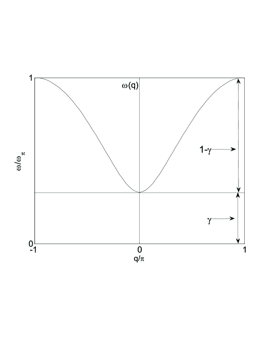
Figure 1: Generalized phonon dispersion, $\omega(q)$, defined in Eq. (20). $(1-\gamma)\omega_{\pi}$ is the phonon ‘band width’ (which vanishes in the Einstein-limit), while $\gamma\omega_{\pi}$ is the phonon ‘mass-gap’ (which vanishes in the Debye-limit). The dispersion parameter, $\gamma$, and the optical phonon frequency, $\omega_{\pi}$, are model parameters.

The introduction of a generalized phonon Hamiltonian avoids the problems associated with hydrodynamic modes and places a criterion on the reliability of the gap-crossing characterization of the critical coupling (as described in Section III.1). Starting from the Heisenberg-SP Hamiltonian in the Einstein limit ($\gamma=1$), the effect of dispersive lattice fluctuations can be investigated via a variation of $\gamma$. The Debye limit is then found via an extrapolation of $\gamma\rightarrow 0$.

The model is solved using the density matrix renormalization group (DMRG) method white with periodic boundary conditions throughout. Our implementation of the DMRG method, including a description of the adaptation of the spin-phonon basis and convergence, is given in the Appendix.

III Results and Discussion

III.1 Gap-crossing

For the Einstein model with a non-vanishing value of $\omega_{E}$ the critical spin-phonon coupling, $g_{\text{c}}$, may be determined using the gap-crossing method of Okamoto and Nomura okamoto , as shown in Fig. 2 for an 80-site chain. If the $N$-site system has quasi-long-range Néel order for $0\leq g\leq g_{\text{c}}(N)$, the lowest excitation is a triplet state, i.e. $\Delta_{\text{st}}<\Delta_{\text{ss}}$ and $\lim_{N\to\infty}\Delta_{\text{st}}=\lim_{N\to\infty}\Delta_{\text{ss}}=0$, where $\Delta_{\text{st}}$ and $\Delta_{\text{ss}}$ are the triplet and singlet gaps, respectively. Conversely, for $g>g_{\text{c}}(N)$, the system is dimerized with a doubly-degenerate singlet GS in the asymptotic limit (corresponding to the translationally equivalent ‘A’ and ‘B’ phases), while the lowest energy triplet excitation is gapped. However, for finite systems the two equivalent dimerization phases mix via quantum tunneling, and now $\Delta_{\text{ss}}<\Delta_{\text{st}}$, with $\lim_{N\to\infty}\Delta_{\text{ss}}=0$ and $\lim_{N\to\infty}\Delta_{\text{st}}>0$. The gap-crossing condition $\Delta_{\text{st}}=\Delta_{\text{ss}}$ therefore defines the finite-lattice crossover coupling $g_{\text{c}}(N)$.

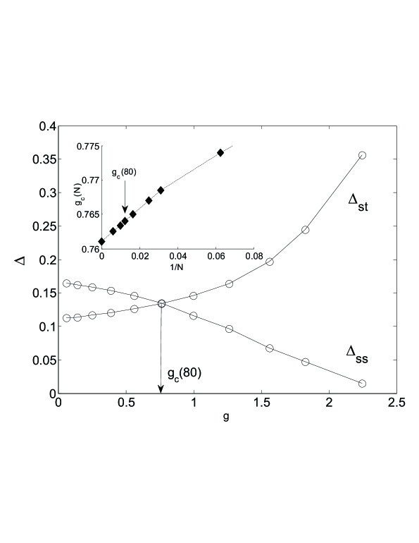
Figure 2: Gap-crossing construction for the $\gamma=1$ (Einstein) Heisenberg-SP model for $N=80$. Inset: The infinite-chain critical coupling $g_{c}^{\infty}$ is determined by extrapolation.

For the Debye model, however, the gap-crossing method fails because of the $q\to 0$ phonons that form a gapless vibronic progression with the groundstate. The hybrid spectrum (shown in Fig. 1) allows us to extrapolate from the pure Einstein limit to the Debye limit, as the lowest vibronic excitation is necessarily $\gamma\omega_{\pi}$. Provided that $\Delta_{\text{ss}}<\omega(q=0)\equiv\gamma\omega_{\pi}$, the gap crossover method unambiguously determines the nature of the GS. We can confidently investigate Eq. (1) for ($0.1\leq\gamma\leq 1$) with $\omega_{\pi}/J\in[1,10]$, thereby determining $g_{\text{c}}(N,\gamma)$. A polynomial extrapolation of $1/N\to 0$ generates the bulk-limit critical coupling $g_{\text{c}}^{\infty}$ for a given $\gamma$ (as illustrated in Fig. 2). A subsequent polynomial extrapolation determines the $\gamma=0$ (Debye) limit. A phase diagram for the Heisenberg-SP chain found in this way is shown in Fig. 3. Notice that for a fixed $\omega_{\pi}$ the critical coupling is larger for the Debye model than for the Einstein model, showing that the quantum fluctuations from the $q<\pi$ phonons (as well as the $q=\pi$ phonon) destablize the Peierls state.

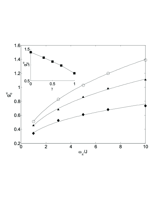
Figure 3: Phase diagram in the $g_{\text{c}}^{\infty}$-$\omega_{\pi}$ plane for the infinite Heisenberg-SP chain for $\gamma=1$ (diamonds) and $\gamma=0.5$ (triangles); extrapolation to $\gamma=0$ generates the Debye-limit (open circles). Inset: variation of $g_{\text{c}}^{\infty}$ with $\gamma$ for the antiadiabatic limit, $\omega_{\pi}/J=10$.

Following Caron and Moukouri caron we tentatively propose a general power-law for the Heisenberg-SP model, relating the bulk-limit critical coupling to $\omega_{\pi}$ for a given $\gamma$,

$$g_{\text{c}}^{\infty}(\omega_{\pi},\gamma)=\beta(\gamma)\omega_{\pi}^{\eta(\gamma)}.$$ (26)

The infinite-chain values of $\beta$ and $\eta$, and $g_{\text{c}}^{\infty}$ for $\omega_{\pi}/J=10$ are given in Table 1. We find a non-zero critical coupling for all phonon regimes $\gamma$, with the absolute value of $g_{\text{c}}^{\infty}$ increasing as $\gamma\to 0$, as shown in the inset of Fig. 3.

$\gamma$	$\beta$	$\eta$	$g_{\text{c}}^{\infty}$
0 (Debye)	0.511	0.437	1.397
0.5	0.452	0.392	1.103
1 (Einstein)	0.350	0.337	0.761

Table 1: Gap-crossing determined bulk-limit values of $\beta(\gamma)$ and $\eta(\gamma)$ (defined by Eq. (26)), and $g_{\text{c}}^{\infty}$ for $\omega_{\pi}/J=10$. The Debye limit ($\gamma=0$) is obtained by extrapolation of $\gamma\to 0$.

III.2 Finite-size scaling

In order to ascertain the analytic behavior of the spin gap from the numerical data it is necessary to account for finite-size effects. We assume that the (singlet-triplet) gap $\Delta_{N}\equiv\Delta_{\text{st}}$ for a finite system of $N$ sites obeys the finite-size scaling hypothesis fisher ; barber

$$\Delta_{N}=\frac{1}{N}F(N\Delta_{\infty}),$$ (27)

with $\Delta_{\infty}$ the spin-gap in the bulk limit. Recalling that $g_{\text{c}}^{\infty}\equiv\lim_{N\to\infty}g_{\text{c}}(N)$, it follows that $\Delta_{\infty}(g_{\text{c}}^{\infty})=0$ and so curves of $N\Delta_{N}$ versus $g$ are expected to coincide at the critical point where the bulk-limit spin-gap vanishes, as confirmed in Fig. 4 and Fig. 5.

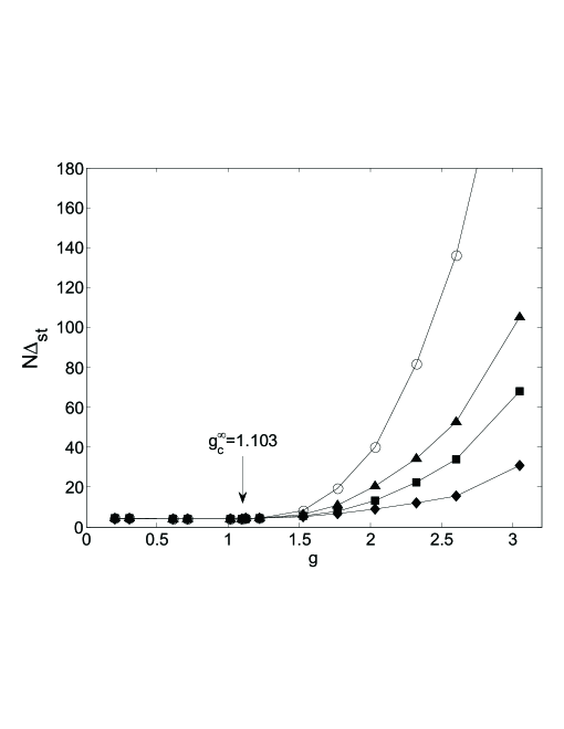
Figure 4: $N\Delta_{\text{st}}(N)$ versus the spin-phonon coupling, $g$, for the $\gamma=0.5$ Heisenberg-SP model for $N=$ $16$ (diamonds), $40$ (squares), $80$ (triangles), and $160$ (open circles) for $\omega_{\pi}/J=10$. The curves converge at $g_{\text{c}}^{\infty}$ (the value shown is obtained via gap-crossing).

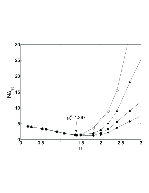
Figure 5: $N\Delta_{\text{st}}(N)$ versus the spin-phonon coupling, $g$, for the $\gamma=0$ (Debye) Heisenberg-SP model for $N=$ $16$ (diamonds), $40$ (squares), $80$ (triangles), and $160$ (open circles) for $\omega_{\pi}/J=10$. The curves converge at $g_{\text{c}}$ (the value shown is obtained via gap-crossing).

The finite-size scaling method is more robust than the gap-crossing approach, being applicable to the SP Hamiltonian for all values of $\gamma$. On the other hand, its use as a quantitative method is limited by the accuracy with which plots may be fitted to Eq. (27). In practice, plots of $N\Delta_{\text{st}}(N)$ versus $g$ become progressively more kinked about the critical point as $\gamma\to 0$. Nevertheless, we find $F$ to be well approximated by a rational function and the resulting $g_{\text{c}}^{\infty}(\gamma)$ to be in accord with the predictions of the gap-crossover method.

III.3 Berezinskii-Kosterlitz-Thouless transition

For a BKT transition the spin-gap $\Delta\equiv\lim_{N\to\infty}\Delta_{\text{st}}$ is expected to exhibit an essential singularity at $g_{\text{c}}^{\infty}$ with plots of $\Delta_{\text{st}}$ versus $g$ for $N\to\infty$ found to be well fitted by the Baxter form baxter (as shown in Fig. 6),

$$\Delta\sim af(g)\exp(-b[f(g)]^{2})$$ (28)

wherebursill ,

$$f(g)\equiv(g-g_{\text{c}}^{\infty})^{-1/2}.$$ (29)

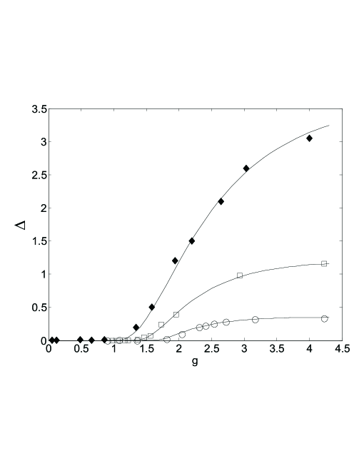
Figure 6: Bulk-limit singlet-triplet gap, $\Delta$, as a function of the spin-phonon coupling, $g$, with $\gamma=1$ (Einstein) [diamonds] $\gamma=0.5$ [open squares] and $\gamma=0$ (Debye) [open circles] for $\omega_{\pi}/J=10$. Plots are fitted to the BKT form (Eq. (28)).

Extrapolating $\Delta_{\text{st}}(N)$ for $1/N\to 0$ generates $\Delta$ for a given $\gamma$ and it is possible, in principle, to distinguish dimerized from spin-fluid GSs by examining the scaling behavior of $\Delta_{\text{st}}(N)$, which tends to zero in the bulk- limit for the spin fluid and to a non-zero $\Delta$ for the gapped phase. However, not only must three parameters ($a$, $b$, and $g_{\text{c}}^{\infty}$) be obtained from a non-linear fit (shown in Table 2), but there is considerable difficulty in determining $\Delta$ accurately near the critical point: the spin-gap is extremely small even for values of $g$ substantially higher than $g_{\text{c}}^{\infty}$ due to the essential singularity in Eq. (28). Determining such small gaps from finite-size scaling is highly problematic with very large lattices required to observe the crossover from the initial algebraic scaling (in the critical regime) to exponential scaling (for gapped systems). Hence the gap-crossover method is expected to be substantially more accurate than a fitting procedure for the determination of the critical coupling, the latter tending to overestimate $g_{\text{c}}^{\infty}$ (see refbursill ), as confirmed by a comparison of Tables 1 and 2.

$\gamma$	$a$	$b$	$g_{\text{c}}^{\infty}$
0	1.014	1.505	1.422
0.5	4.110	2.101	1.120
1	14.206	3.042	0.731

Table 2: Baxter-equation parameters obtained by fits to Eq. (28) for $\omega_{\pi}/J=10$.

III.4 Correlation functions and order parameters

The $q=\pi$ structure factor, $S(q)$, of the bond-order auto-correlation function can be used to determine the phase transition. $S(q)$ is defined by,

$$S(q)=\sum_{m}\exp(iqm)\langle C(m)\rangle$$ (30)

where

$$C(m)=\frac{1}{N}\sum_{l}(O_{l}-\langle O_{l}\rangle)(O_{l+m}-\langle O_{l+m}\rangle).$$ (31)

The ‘bond order’ operator, $O_{l}$, is given by

$$O_{l}=\left\{\begin{array}[]{ll}S_{l}^{z}S_{l+1}^{z}&\mbox{spin-spin};\\ (q_{l}-q_{l+1})&\mbox{phonon displacement}.\end{array}\right.$$

The transition to a dimerized state is marked by the development of a staggered kinetic energy modulation and quasi long-range-order in the bond order. It is signalled by a divergent peak in $S(q=\pi)$ at the critical coupling in the asymptotic limit, as shown in Fig. 7. (We note, however, that the structure factor associated with the phonon displacement bond order auto-correlator, $O_{l}=(q_{l}-q_{l+1})$, fails to resolve the transition, instead increasing monotonically with $g$ for all $\gamma$.)

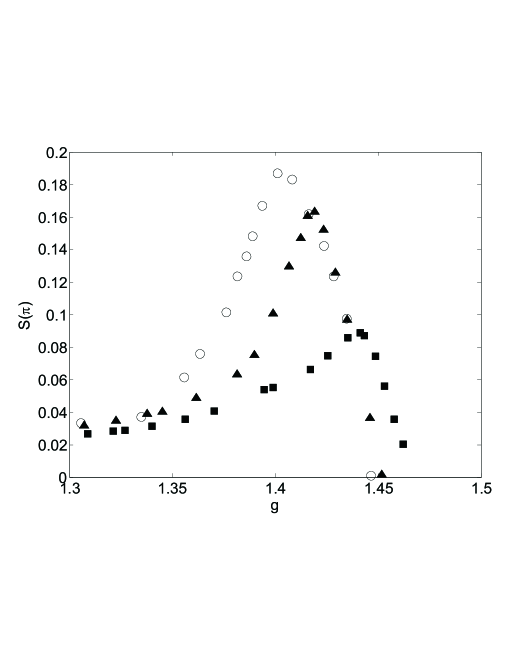
Figure 7: Structure factor for the spin-spin bond order auto-correlation function at $q=\pi$ for the $\gamma=0$ (Debye) model with $\omega_{\pi}/J=10$ for $N$=20 (squares), $N$=40 (triangles), and $N$=80 (open circles).

Following barford1 ; barford2 we also consider staggered spin-spin, $m_{\text{s}}$, and phonon displacement, $m_{\text{p}}$, order parameters,

$$m_{\text{s}}=\frac{1}{N}\sum_{l}(-1)^{l}\langle S^{z}_{l}S^{z}_{l+1}\rangle$$ (32)

and

$$m_{\text{p}}=\frac{1}{N}\sum_{l}(-1)^{l}\langle B_{l+1}-B_{l}\rangle.$$ (33)

For linear chains under OBC, the end sites break the energetic degeneracy between the otherwise equivalent $|A\rangle$ and $|B\rangle$ states, which are related by a translation of one repeat unit. Physically, however, PBC are strongly preferable to OBC as boundary effects are eliminated and finite-size extrapolations can be performed for much smaller $N$. In addition, greater accuracy can be obtained by investigating cyclic chains, although it is necessary to explicitly break the degeneracy between the ‘A’ and ‘B’ phases through inclusion of a symmetry-breaking term $H^{\prime}$ in Eq. (1),

$$H^{\prime}=\rho\sum_{l}(-1)^{l}\langle\textbf{S}_{l}\cdot\textbf{S}_{l+1}\rangle,$$ (34)

and extrapolating $\rho\to 0$.

Our results indicate that both $m_{\text{s}}$ and $m_{\text{p}}$ scale to zero as $g\to\infty$, suggesting $g_{\text{c}}^{\infty}=0^{+}$ for all $\gamma$, accounting for the earlier findings ofbarford1 . These predictions are incomplete deviation to the other positive signatures of a phase transition for $g>0$. We attribute this discrepancy to the action of the perturbation $H^{\prime}$ (Eq. (34)) on the fixed-point behavior of the Heisenberg-SP Hamiltonian for an insufficiently small perturbation, and thus conclude that the staggered order parameters must be treated with caution when determining the phase transition.

III.5 Quantum bipartite entanglement

It has recently been conjectured that quantum entanglement plays an important role in the quantum phase transitions (QPT) of interacting quantum lattices. At the critical point—as in a conventional thermal phase transition—long-range correlations pervade the system. However, because the system is at $T=0$ (and assuming no ground-state degeneracy) the GS is necessarily a pure state. It follows, then, that the onset of (long-range) correlations – being the principal experimental signature of a QPT – is due to entanglement in the GS on all length scales.

For an $N$-site lattice, bipartite entanglement is quantified through the von Neumann entropy vne ,

$$S_{L}=-\mbox{Tr}_{\bar{S}}\rho_{S}(L)\log_{2}\rho_{S}(L)=-\sum_{\alpha}\nu_{\alpha}\log_{2}\nu_{\alpha},$$ (35)

where $\rho_{S}(L)$ is the reduced-density matrix of an $L$-site block (typically coupled to an $L$-site environment $\bar{S}$ such that $2L=N$) and the $\nu_{\alpha}$ are the eigenvalues of $\rho_{S}(L)$. It is clear from Eq. (35) that a slow decay of the reduced density-matrix eigenvalues corresponds to a large block entropy. Provided the entanglement is not too great and the $\nu_{\alpha}$ decay rapidly, a matrix-product state is then a good approximation to the GS scholl . We note here the utility of the DMRG prescription in determining $S_{L}\equiv S_{N/2}$ noack .

Wu et al. wu argued, quite generally, that QPTs are signalled by a discontinuity in some entanglement measure of the infinite quantum system. For finite one-dimensional gapped systems the noncritical entanglement is characterized by the saturation of the von Neumann entropy with increasing $L$: the entropy of entanglement either (i) vanishes for all $L$ or (ii) grows monotonically with $L$ until it reaches a saturation value for some block length $L_{0}$ vidal . Noncritical entanglement in the GS corresponds, thus, to a weak, semi-local entang1 form of entanglement driven by the appearance of a length scale $L_{0}$ due to, e.g, a mass gap in the Hamiltonian. For any $L$, the reduced-density matrix $\rho_{S}(L)$ is effectively supported on just a small, bounded subspace of the $L$-spin Hilbert space. Critical models, on the other hand, are expected to exhibit logarithmic divergence in $S_{L}$ at large $L$: $S_{L}=k\log_{2}L+\mbox{constant}$.

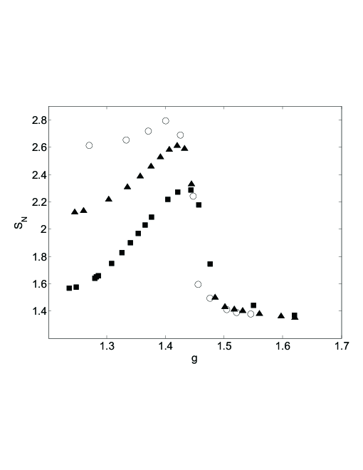
Figure 8: Von Neumann entropy, $S_{L}$, for the $\gamma=0$ (Debye) model with $\omega_{\pi}/J=10$ for lattice sizes $N=20$ (squares), $40$ (triangles), and $80$ (open circles); $L=N/2$.

For a given total system size $N$ and phonon dispersion $\gamma$, the block entropy is found to be maximal for a non-zero spin-phonon coupling $g_{\text{c}}(N)$, close to the corresponding gap-crossing and bond order structure factor values (as shown in Table 3). As shown in Fig. 8, in the critical regime, $g<g_{\text{c}}(N)$, the block entropy is indeed found to scale logarithmically with system-block length, while in the gapped phase, $g>g_{\text{c}}(N)$, it is characterized by the emergence of a saturation length scale $L_{0}$ that varies with $\gamma$. These findings are in agreement with vidal and consistent with the observation that the transition belongs to the BKT universality classkt .

$N$	$g_{\text{c}}^{\text{gap}}$	$g_{\text{c}}^{\text{SF}}$	$g_{\text{c}}^{\text{vN}}$
20	1.441	1.441	1.443
40	1.419	1.420	1.422
80	1.400	1.402	1.403

Table 3: Consistency of the various probes of the transition: critical spin-phonon couplings determined by gap-crossing (gap), $q=\pi$ structure factor of the bond order auto-correlation function (SF), and von Neumann entropy (vN) for $N=20$, $40$, and $80$ sites. $\gamma=0$ (Debye) and $\omega_{\pi}/J=10$.

III.6 Phase diagram

To conclude this section we discuss the phase diagram of the Heisenberg spin-Peierls model. Fig. 3 shows the phase diagram as a function of the model parameters $g$ and the $q=\pi$ phonon gap, $\omega_{\pi}$, as defined in Eq. (17) and Eq. (19). Evidently, for a fixed value of $\omega_{\pi}$ the spin-Peierls state is less stable to dispersive, gapless quantum lattice fluctuations than to gapped, non-dispersive fluctuations, implying that the $q<\pi$ phonons also destablize the Peierls state.

It is also instructive, however, to plot the phase diagram as a function of the physical parameters $\alpha$ and ${\omega_{b}}=\sqrt{K/M}$, as defined in Eq. (2), Eq. (3) and Eq. (4). The mapping between model and physical parameters is achieved via Eq. (10), Eq. (14), Eq. (24), and Eq. (25) (and setting $K=1$). Since $\omega_{\pi}={\omega_{b}}$ for the Einstein model, whereas $\omega_{\pi}=2{\omega_{b}}$ for the Debye model, the Debye model is further into the antiadiabatic regime for a fixed value of ${\omega_{b}}$. We also note that for a given model electron-phonon coupling parameter, $g$, the physical electron-phonon coupling parameter, $\alpha$, is larger in the Debye model than the Einstein model (see Eq. (10) and Eq. (14)). Consequently, we expect the dimerized phase to be less robust to quantum fluctuations in the Debye model for fixed values of ${\omega_{b}}$ and $\alpha$, as confirmed by Fig. 9footnote1 .

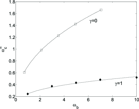
Figure 9: Phase diagram in the $\alpha_{c}^{\infty}$-${\omega_{b}}$ plane for the infinite Heisenberg-SP chain for $\gamma=1$ (Einstein), diamonds; and $\gamma=0$ (Debye), squares.

IV Conclusions

The coupling of spin and lattice degrees of freedom with reduced dimensionality results in the instability of a one-dimensional Luttinger liquid towards lattice dimerization and the opening of a gap at the Fermi surface. Coupling to the lattice gives rise to a BKT transition from a spin liquid with gapless spinon excitations to a dimerized phase characterized by an excitation gap.

For the quantum Heisenberg chain in the antiadiabatic limit ($J/\omega_{\pi}<<1$), the spin-fluid phase becomes unstable with respect to lattice dimerization above a non-zero spin-phonon-coupling threshold for all phonon gaps, $\gamma\omega_{\pi}$. This observation holds for $\omega_{\pi}/J\sim 1$. Increasing the contribution of dispersive phonons to $H_{\text{p}}$ gives rise to an increase in the critical coupling, supporting the intuition that gapless phonons more readily penetrate the GS (with the $q<\pi$ phonon modes renormalizing the dispersion at the Peierls-active modes). This observation has been corroborated by an array of independent verifications. The behavior of the Debye model is qualitatively different from the Einstein model, with different exponents and prefactors for the critical coupling versus phonon frequency, Eq. (26), and the Baxter expression for the spin-gap, Eq. (28).

We note that staggered order parameters are an unreliable means of determining the phase transitionbarford1 , because of the use of a symmetry breaking perturbation for PBCs that changes the FP of the Hamiltonian for insufficiently small perturbations.

Placing these findings in the context of experiment, estimates of the model parameters for a number of spin-Peierls compounds are listed in Table 4 (reproduced from bursill ). Clearly, the static approximation is not applicable to CuGeO₃. In addition, it is also questionable as to whether the listed organic spin-Peierls compounds are themselves truly static lattice materials, thereby justifying a dynamical phonon treatment. The most physically relevant region of the phonon spectrum, however, appears to be one of intermediate frequency, dividing the adiabatic and antiadibatic limits. Nevertheless, even though $\omega_{\pi}/J=3$ for CuGeO₃, referring to the phase diagram of Fig. 3 we note the applicability of the generalized power-law for small $\omega_{\pi}/J$, and hence the occurrence of a finite critical coupling in the regime applicable to CuGeO₃.

Material	$J$	$\omega_{\pi}$	$\Delta$
CuGeO3	100	300	20
TTFCuS4C4(C3F)4	70	10*	20
(MEM)(TCNQ)2	50	100	60

Table 4: Estimates of the antiferromagnetic exchange, $J$, dimerization phonon frequency, $\omega_{\pi}$, and spin gap, $\Delta$, for various SP materials. All units are in Kelvins. *Value deduced by comparison of experimental values of $J$, the transition temperature, and $\Delta$ to mean-field theoretical expressions in kasper .

Examination of intermediate phonon frequencies and their extension to spinful fermion models with Coulomb repulsionbarford2 is straightforward and currently in progress.

Appendix A DMRG and in situ optimization

We solve Eq. (17) and Eq. (18) using the real-space density matrix renormalization group (DMRG) method white , with ten oscillator levels per site, typically $\sim 200$ block states and ca.  $10^{6}$ superblock states. Finite lattice sweeps are performed at target chain lengths under PBC. The convergence indicators are shown in Tables 5-9, with additional convergence tables in refbarford1 for the same model.

The DMRG algorithm typically proceeds through the augmentation of an $(L-1)$-site system block $S$ by a single site $i_{a}$. The augmented system block $S^{\prime}$ ($L$ sites) is coupled to an augmented $L$-site environment block $E^{\prime}$, formed analogously to $S^{\prime}$. The system and environment comprise the superblock ($2L=N$ sites), whose state vector, $|\Psi\rangle$, is readily obtained by a suitable diagonalization routine. By tracing over the degrees of freedom in $E^{\prime}$, the reduced-density matrix of $S^{\prime}$ ($\rho_{S^{\prime}}(L)=\mbox{Tr}_{E^{\prime}}|\Psi\rangle\langle\Psi|$) is obtained; a pre-determined proportion of the largest-eigenvalue eigenstates of $\rho_{S^{\prime}}(L)$ is retained, forming the system-block basis for the next iteration. The DMRG prescription results in $\mathcal{O}(N)$-growth of the superblock Hilbert space.

In addition (and prior) to the effective truncation and rotation of the system-block basis, we employ a single-site optimization at each DMRG step. All superblock degrees of freedom, save those belonging to $i_{a}$, are traced over and the resulting single-site reduced-density matrix $\rho_{a}$ is diagonalized, generating an optimal single-site basis in the correct physical environment with which to augment $S$ lav ; barford1 ; barford2 ; jeck ; zhang . This local Hilbert space adaptation generates single-site bases, the principal utility of which is the solution of many-body problems with large numbers of degrees of freedom. A controlled truncation of a large Hilbert space therefore allows a small (for our purposes six-dimensional) optimal basis to be used without significant loss of accuracy, making it ideally suited to spin-phonon problems, where the number of phonons is not conserved and the phonon Hilbert space is, in principle, infinite.

$m$	$E_{g}/J$	$n_{l}$	$\sigma_{n}$
2	-18.746372	0.00291	0.0468
5	-18.747323	0.00221	0.0470
8	-18.747323	0.00221	0.0470
10	-18.747367	0.00221	0.0470

Table 5: GS energy, $E_{g}/J$, average phonon occupation number, $n_{l}=\langle b_{l}^{\dagger}b_{l}\rangle$, and standard deviation, $\sigma_{n}$, for a 40-site chain with $\gamma=1$ (Einstein), $\omega_{\pi}/J=10$, and $m$ oscillator levels per site.

$m$	$E_{g}/J$	$n_{l}$	$\sigma_{n}$
2	-27.198068	0.0331	0.179
5	-31.795996	0.1477	0.437
8	-31.991408	0.1717	0.481
10	-31.991541	0.1719	0.484

Table 6: GS energy, $E_{g}/J$, average phonon occupation number, $n_{l}$, and standard deviation, $\sigma_{n}$, for a 40-site chain with $\gamma=0$ (Debye), $\omega_{\pi}/J=10$, and $m$ oscillator levels per site.

$m$	$E_{g}/J$	$n_{l}$	$\sigma_{n}$
2	-18.882263	0.0318	0.175
5	-19.358486	0.1368	0.420
8	-19.371279	0.1520	0.451
10	-19.371877	0.1522	0.452

Table 7: GS energy, $E_{g}/J$, average phonon occupation number, $n_{l}$, and standard deviation, $\sigma_{n}$, for a 40-site chain with $\gamma=0$ (Debye), $\omega_{\pi}/J=1$, and $m$ oscillator levels per site.

$\epsilon$	$E_{g}/J$	$M$	SBHSS
$10^{-10}$	-24.266060	176	14572
$10^{-11}$	-24.350806	278	32328
$10^{-12}$	-24.377641	300	60054
$10^{-15}$	-24.377646	350	172654

Table 8: GS energy, $E_{g}/J$, of Heisenberg-SP model as a function of the density-matrix eigenvalue product cutoff, $\epsilon$, number of system block states, $M$, and the superblock Hilbert space size, (SBHSS) for a 40-site chain with 10 oscillator levels per site and $\gamma=0.5$.

$N$	$\epsilon$	$\Delta_{\text{ss}}$	$\Delta_{\text{st}}$
8	$10^{-12}$	0.924728	0.513871
8	$10^{-15}$	0.924726	0.513869
8	$10^{-20}$	0.924726	0.513869
20	$10^{-12}$	0.343794	0.215902
20	$10^{-14}$	0.343792	0.215900
20	$10^{-16}$	0.343792	0.215899
40	$10^{-12}$	0.183655	0.113428
40	$10^{-13}$	0.183641	0.113405
40	$10^{-14}$	0.183640	0.113403
40	$10^{-15}$	0.183640	0.113403
160	$10^{-12}$	0.046367	0.030776
160	$10^{-13}$	0.046163	0.030550
160	$10^{-14}$	0.046161	0.030528
160	$10^{-15}$	0.046163	0.030526

Table 9: DMRG convergence of the singlet, $\Delta_{\text{ss}}$, and triplet, $\Delta_{\text{st}}$, gaps of the Heisenberg-SP model for $\gamma=0$ with density-matrix eigenvalue product cutoff, $\epsilon$, for various $N$-site periodic lattices, where $\omega_{\pi}/J=10$ and $g=0.4$

- (1) R. Peierls, Quantum Theory of Solids (Oxford University Press, Oxford, 1955).
- (2) J. W. Bray, H. R. Hart, Jr., L. V. Interrante, I. S. Jacobs, J. S. Kasper, G. D. Watkins, S. H. Wee, and J. C. Bonner, Phys. Rev. Lett. 35, 774 (1975).
- (3) R. H. McKenzie and J. W. Wilkins, Phys. Rev. Lett. 69, 1085 (1992).
- (4) A. Weisse, H. Fehske, G. Wellein, A. R. Bishop, Phys. Rev. B 62, R747 (2000).
- (5) W. Barford, R. J. Bursill, and M. Y. Lavrentiev, Phys. Rev. B 65, 075107 (2002).
- (6) M. Hase, I. Terasaki, and K. Uchinokura, Phys. Rev. Lett. 70, 3651 (1993).
- (7) D. Augier and D. Poilblanc, Eur. Phys. J. B 58, 9110 (1998)
- (8) G. Wellein, H. Fehske, and A. P. Kampf, Phys. Rev. Lett. 81, 3956 (1998).
- (9) R. J. Bursill, R. H. McKenzie and C. J. Hamer, Phys. Rev. Lett. 83, 408 (1999).
- (10) R. Citro, E. Orignac, and T. Giamarchi, Phys. Rev. B 72, 024434 (2005).
- (11) L. G. Caron and S. Moukouri, Phys. Rev. Lett. 76, 4050 (1996).
- (12) K. Kuboki and H. Fukuyama, J. Phys. Soc. Jpn. 56, 3126 (1987).
- (13) H. Bakrim and C. Bourbonnais, Phys. Rev. B 76, 195115 (2007).
- (14) E. Fradkin and J. E. Hirsch, Phys. Rev. B 27, 1680 (1983).
- (15) G. T. Zimanyi, S. A. Kivelson, and A. Luther, Phys. Rev. Lett. 60, 2089 (1988); G. T. Zimanyi and S. A. Kivelson, Mol. Cryst. Liq. Cryst. 160, 457 (1988).
- (16) W. Barford and R. J. Bursill, Phys. Rev. Lett. 95, 137207 (2005).
- (17) See, for example, C. Kittel (p. 25), Quantum Theory of Solids (Wiley, 1987).
- (18) S. R. White, Phys. Rev. Lett. 69, 2863 (1992); Phys. Rev. B 48, 10345 (1993).
- (19) K. Okamoto, K. Nomura, Phys. Lett. A 169, 433 (1992).
- (20) M. E. Fisher and M. N. Barber, Phys. Rev. Lett. 28, 1516 (1972).
- (21) C. J. Hamer and M. N. Barber, J. Phys. A 14, 241 (1981).
- (22) R. J. Baxter, J. Phys. C 6, L94 (1973).
- (23) W. Barford and R. J. Bursill, Phys. Rev. B 73, 045106 (2006).
- (24) C. H. Bennett, H. J. Bernstein, S. Popescu, and B. Schumacher, Phys. Rev. A 53, 2046 (1996).
- (25) U. Schollwock, Rev. Mod. Phys. 77, 259 (2005).
- (26) C. Mund, Ö. Legeza, and R. M. Noack, Phys. Rev. B 79, 245130 (2009).
- (27) L.-A. Wu, S. Bandyopadhyay, M. S. Sarandy, and D. A. Lidar, Phys. Rev. A 72, 032309 (2005).
- (28) G. Vidal, Phys. Rev. Lett. 99, 220405 (2007).
- (29) A good approximation to can be obtained by diagonalizing the Hamiltonian corresponding to the system block and only a few extra, neighboring/environment-block spins, e.g. DMRG.
- (30) J. M. Kosterlitz and D. J. Thouless, J. Phys C 6, 1181, (1973).
- (31) Relative to the Einstein limit, the phase diagram for the Debye limit for physical parameters corresponds to stretching the y-axis and contracting the x-axis of Fig. 3.
- (32) J. S. Kasper and D. E. Moncton, Phys. Rev B 20, 2341 (1979).
- (33) E. Jeckelmann, C. Zhang, and S. R. White, Phys. Rev. B 60, 7950 (1999).
- (34) C. Zhang, E. Jeckelmann, and S. R. White, Phys. Rev. B 60, 14092 (1999).