Gravito-electromagnetic Aharonov-Bohm effect: some rotation effects revised

Abstract

By means of the description of the standard relative dynamics in terms of gravito-electromagnetic fields, in the context of natural splitting, we formally introduce the gravito-magnetic Aharonov-Bohm effect. Then, we interpret the Sagnac effect as a gravito-magnetic Aharonov-Bohm effect and we exploit this formalism for studying the General Relativistic corrections to the Sagnac effect in stationary and axially symmetric geometries.

1 Introduction

In a previous paper[1] we developed a formal approach, for the description of the relativistic dynamics, which lead to what we called gravito-magnetic Aharonov-Bohm effect. This approach is based on the description of the standard relative dynamics in the context of the natural splitting, introduced by Cattaneo and subsequently developed by himself, Ferrarese and collaborators. The formulation that we gave of the gravito-magnetic Aharonov-Bohm effect holds in exact theory, and it generalizes some old results obtained at first order approximation[3]. In the previous paper we used this approach to calculate the Sagnac time delay, for matter or light beams counter-propagating in a rotating reference frame in flat space-time. In doing so, we exploited the formal analogy between matter (or light) beams counter propagating in circular trajectories in gravitational or inertial fields, and charged beams propagating in a region where a magnetic potential is present. Here we apply the formalism of the gravito-magnetic Aharononv-Bohm effect for studying the Sagnac effect in curved space-time. Tartaglia[4] studied the General Relativistic corrections to the Sagnac effect in Kerr space-time, while an approach similar to ours, i.e. based on a gravito-magnetic Aharonov-Bohm effect, was developed by Cohen and Mashhoon[5], who studied the gravito-magnetic time delay in the weak gravitational field of a rotating source, at first order approximation. Our formalism allows to generalize these results to arbitrary stationary and axially symmetric geometries, in full theory without any approximations.

The paper is organized as follows: in Section 2 we recall the main features of the gravito-magnetic description of dynamics, in Sections 3 and 4 we illustrate, respectively, the Aharonov-Bohm effect and the gravito-magnetic Aharonov-Bohm effect. In Section 5 we study the Sagnac effect in flat and curved space-time.

2 Gravito-electromagnetic description of relativistic dynamics

By applying Cattaneo’s splitting, the dynamics of massive or massless particles, relative to a given time-like congruence $\Gamma$ of unit vectors $\bm{\gamma}(x)$, can be described in terms of a ”gravito-electromagnetic” analogy. Here we briefly review the main features of this approach, in order to formulate, in the following Sections, the gravito-magnetic Aharonov-Bohm effect. The details of the calculations may be found in [2].

The congruence $\Gamma$ defines the physical reference frame with respect to which the particles move, and an observer at rest on this physical frame has a world-line which coincides with one of the world-lines of the congruence.

Let $\gamma^{\mu}$ be the components of the unit vectors field $\bm{\gamma}(x)$ in coordinates adapted to the congruence. Their expression in terms of the metric tensor $g_{\mu\nu}$ is

$$\left\{\begin{array}[]{l}\gamma^{{0}}=\frac{1}{\sqrt{-g_{{00}}}}\\ \gamma^{i}=0\end{array}\right.\;\;\;\;\;\;\;\;\;\;\;\;\left\{\begin{array}[]{l}\gamma_{0}=-\sqrt{-g_{{00}}}\\ \gamma_{i}=g_{i{0}}\gamma^{{0}}\end{array}\right.$$ (1)

Then, if we introduce the gravito-electric potential $\phi^{G}$ and the gravito-magnetic potential $\tilde{A}_{i}^{G}$, defined by

$$\left\{\begin{array}[]{c}\phi^{G}\doteq-c^{2}\gamma^{0}\\ \widetilde{A}_{i}^{G}\doteq c^{2}\frac{\gamma_{i}}{\gamma_{0}}\end{array}\right.$$ (2)

we can write the gravito-magnetic field

$$\widetilde{B}_{G}^{i}\doteq\left(\widetilde{{\bf\nabla}}\times\bm{\tilde{A}}_{G}\right)^{i}$$ (3)

and the gravito-electric field:

$$\widetilde{E}^{G}_{i}\doteq-\left(-\widetilde{\partial}_{i}\phi_{G}-\partial_{0}\widetilde{A}^{G}_{i}\right)$$ (4)

in analogy with the definitions of classical electromagnetism. Notice that we used the following differential operator

$$\tilde{\partial}_{\mu}\doteq\partial_{\mu}+\gamma_{\mu}\gamma^{0}\partial_{0}$$ (5)

which is called transverse partial derivative, and it defines the space-projection of the local gradient; furthermore, we recall here that the ” $\tilde{}$ ” denotes space-vectors, i.e. vectors that are obtained by projecting the world-vectors onto the 3-dimensional subspace orthogonal to the time-like direction spanned by $\gamma^{\mu}$ (see the following Remark).

Remark  Let $\mathcal{M}^{4}$ be a (pseudo)riemannian manifold $\mathcal{M}^{4}$, that is a pair $\left(\mathcal{M},\mathbf{g}\right)$, where $\mathcal{M}$ is a connected 4-dimensional Haussdorf manifold and $\mathbf{g}$ is the metric tensor. $\mathcal{M}^{4}$ is the mathematical model of the physical space-time. At each point $p\in\mathcal{M}^{4}$, the tangent space $T_{p}$ can be split into the direct sum of two subspaces: $\Theta_{p}$, spanned by $\gamma^{\mu}$, which we shall call local time direction of the given frame, and $\Sigma_{p}$, the 3-dimensional subspace which is supplementary (orthogonal) with respect to $\Theta_{p}$; $\Sigma_{p}$ is called local space platform of the given frame. So, the tangent space can be written as the direct sum

$$T_{p}=\Theta_{p}\oplus\Sigma_{p}$$ (6)

Let $\{\bm{e}_{\mu}\}$ be a basis of $T_{p}$. A vector $\bm{v}=v^{\mu}\bm{e}_{\mu}\in T_{p}$ can be projected onto $\Theta_{p}$ and $\Sigma_{p}$ using the time projector

$$P_{\Theta}\doteq-\gamma_{\mu}\gamma_{\nu}$$ (7)

and the space projector

$$P_{\Sigma}\doteq\gamma_{\mu\nu}\doteq g_{\mu\nu}+\gamma_{\mu}\gamma_{\nu}$$ (8)

in the following way:

$$\left\{\begin{array}[]{rclll}\bar{v}_{\mu}&\equiv&P_{\Theta}\left(\,v_{\mu}\right)&\doteq&-\gamma_{\mu}\gamma_{\nu}v^{\nu}\\ \widetilde{v}_{\mu}&\equiv&P_{\Sigma}\left(\,v_{\mu}\right)&\doteq&\gamma_{\mu\nu}v^{\nu}=\left(g_{\mu\nu}+\gamma_{\mu}\gamma_{\nu}\right)v^{\nu}=v_{\mu}+v^{\nu}\gamma_{\nu}\gamma_{\mu}\end{array}\right.$$ (9)

From Eq. (9), $\forall\bm{v}\in T_{p}$ we have

$$v_{\mu}=\bar{v}_{\mu}+\widetilde{v}_{\mu}=P_{\Theta}(v_{\mu})+P_{\Sigma}(v_{\mu})$$ (10)

This defines the natural splitting of a vector $\bm{v}$. $\square$

In terms of the physical quantities that we have introduced so far, the space projection of the geodesics equation for matter or massless particles can be written in the form

$$\frac{\hat{D}\widetilde{p}_{i}}{dT}=m\widetilde{E}^{G}_{i}+m\gamma_{0}\left(\frac{\bm{\tilde{v}}}{c}\times\bm{\tilde{B}}_{G}\right)_{i}$$ (11)

For particles of rest mass $m_{0}$, $m$ is defined by

$$m\doteq\frac{m_{0}}{\sqrt{1-\frac{\widetilde{v}^{2}}{c^{2}}}}$$ (12)

and it is the standard relative mass, which depends on their standard relative velocity $\bm{\tilde{v}}$. For massless particles (such as photons) $m$ is proportional to the standard relative energy, and it is defined by

$$m=\frac{h\nu}{c^{2}}$$ (13)

in terms of the frequency $\nu$ and the Planck constant. In Eq. (11) $dT$ is the standard relative time interval

$$dT=-\frac{1}{c}\gamma_{\mu}dx^{\mu}$$ (14)

and it represents the proper time interval as measured by an observer at rest in $\Gamma$.

Eq. (11) shows that the variation of the standard relative momentum vector $\tilde{p}_{i}$ (in terms of a suitable derivative operator $\frac{\hat{D}}{dT}$) is determined by the action of a gravito-electromagnetic Lorenz force. By means of Eq. (11) we may give a description of the relativistic dynamics in analogy with the electromagnetic theory. This description has been obtained without any approximations, consequently it applies to arbitrary congruences, in both flat and curved space-time. Of course, if one performs a first order approximation, the gravito-electromagnetic analogy that we have obtained corresponds to the well known gravito-electromagnetic description of the weak field approximation of General Relativity (see for instance [7],[8],[9]).

If the particles are not free, but are acted upon by an external force field $F^{\alpha}$, Eq. (11) becomes

$$\frac{\hat{D}\widetilde{p}_{i}}{dT}=m\widetilde{E}^{G}_{i}+m\gamma_{0}\left(\frac{\bm{\tilde{v}}}{c}\times\bm{\tilde{B}}_{G}\right)_{i}+\widetilde{F}_{i}$$ (15)

where the space projection $\widetilde{F}_{i}$ of the external field has been introduced. For instance, the constraints that force a particle to move along a circular path (or guide) are external fields: this is what happens to beams of particles that propagate in a rotating ring interferometer, which is the typical situation of the Sagnac effect.

We recall here that the gravito-magnetic effects are related to the rotational features of the congruence we deal with. In fact, starting from the definition of space vortex tensor of the congruence $\Gamma$

$$\widetilde{\Omega}_{\mu\nu}=\gamma_{0}\left[\widetilde{\partial}_{\mu}\left(\frac{\gamma_{\nu}}{\gamma_{0}}\right)-\widetilde{\partial}_{\nu}\left(\frac{\gamma_{\mu}}{\gamma_{0}}\right)\right]$$ (16)

we may define and axial 3-vector $\tilde{\omega}^{i}$, by means of the relation

$$\widetilde{\omega}^{i}\doteq\frac{c}{4}\varepsilon^{ijk}\tilde{\Omega}_{jk}=\frac{c}{2}\varepsilon^{ijk}\gamma_{0}\tilde{\partial}_{j}\left(\frac{\gamma_{k}}{\gamma_{0}}\right)$$ (17)

where

$$\varepsilon^{ijk}\doteq\frac{1}{\sqrt{det(\gamma_{ij})}}\epsilon^{ijk}$$

is the Ricci-Levi-Civita tensor density, defined in terms of the completely antisymmetric Ricci-Levi-Civita tensor $\epsilon^{ijk}$ and of the space metric tensor $\gamma_{ij}$. The gravito-magnetic field $\widetilde{B}_{G}^{i}$ is proportional to this vector:

$$\widetilde{\omega}^{i}=\frac{1}{2c}\gamma_{0}\widetilde{B}_{G}^{i}$$ (18)

This means that, for instance, when we deal with a congruence of rotating observers, or when we deal with a congruence of observers around a rotating source of gravitational field, we do expect gravito-magnetic effects to appear.

3 The Aharonov-Bohm effect

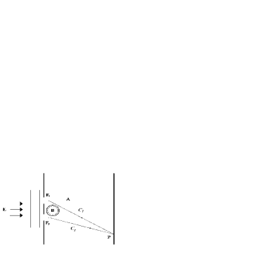
Figure 1: A single coherent charged beam, originating in $E$, is split into two parts (passing through the two slits $F_{1}$ and $F_{2}$) that propagate, respectively, along the paths $C_{1}$ and $C_{2}$ (in the figure these paths are represented, respectively, by $EF_{1}P$ and $EF_{2}P$). Between the paths a solenoid is present; the magnetic field $\bm{\vec{B}}$ is entirely contained inside the solenoid, while outside there is a constant vector potential $\bm{\vec{A}}$. In $P$, the beams interfere and an additional phase shift, provoked by the magnetic field confined inside the solenoid, is observed.

Consider the two slits experiment (see Figure 1) and imagine that a single coherent charged beam is split into two parts, which travel in a region where only a magnetic field is present, described by the 3-vector potential $\bm{\vec{A}}$; then the beams are recombined to observe the interference pattern. The phase of the two wave functions, at each point of the pattern, is modified, with respect to the case of free propagation ($\bm{\vec{A}}~{}=~{}0$), by the magnetic potential. The magnetic potential-induced phase shift has the form[10]

$$\Delta\Phi=\frac{e}{c\hbar}\oint_{C}\bm{\vec{A}}\cdot{\rm d}\bm{\vec{x}}=\frac{e}{c\hbar}\int_{S}\bm{\vec{B}}\cdot{\rm d}\bm{\vec{S}}$$ (19)

where $C$ is the oriented closed curve, obtained as the sum of the oriented paths $C_{1}$ and $C_{2}$ relative to each component of the beam. Eq. (19) expresses (by means of Stoke’s Theorem) the phase difference in terms of the flux of the magnetic field across the surface $S$ enclosed by the curve $C$. Aharonov and Bohm[10] applied this result to the situation in which the two split beams pass one on each side of a solenoid inserted between the paths. Thus, even if the magnetic field $\bm{\vec{B}}$ is totally contained within the solenoid and the beams pass through a $\bm{\vec{B}}~{}=~{}0$ region, a resulting phase shift appears, since a non null magnetic flux is associated to every closed path which encloses the solenoid.

Tourrenc[11] showed that no explicit wave equation is demanded to describe the Aharonov-Bohm effect, since its interpretation is a pure geometric one: in fact Eq. (19) is independent of the physical nature of the interfering charged beams, which can be spinorial, vectorial or tensorial. So, if we deal with relativistic charged beams, their propagation is described by a relativistic wave equation, such as the Dirac equation or the Klein-Gordon equation, depending on the nature of the beams themselves. From a physical viewpoint, spin has no influence on the Aharonov-Bohm effect because there is no coupling with the magnetic field which is confined inside the solenoid. Moreover, if the magnetic field is null, the Dirac equation is equivalent to the Klein-Gordon equation, and this is the case of a constant potential. As far as we are concerned, since in what follows we neglect spin, we shall just use Eq. (19) and we shall not explicitly refer to any relativistic wave equation.

Indeed, things are different when a particle with spin, moving in a rotating frame or around a rotating mass, is considered. In this case a coupling between the spin and the angular velocity of the frame or the angular momentum of the rotating mass appears (this effect is evaluated by Hehl-Ni[12], Mashhoon[13] and Papini[14]). Hence, the formal analogy leading to the formulation of the gravito-magnetic Aharonov-Bohm effect, which is outlined in the following Section, holds only when the spin-rotation coupling is neglected.

4 The Gravito-magnetic Aharonov-Bohm effect

In this Section, on the basis of the gravito-electromagnetic description of the relativistic dynamics that we recalled before, we introduce the gravito-magnetic Aharonov-Bohm effect. This enables us to outline an analogy between matter (or light) beams, counter-propagating around circular orbits, in stationary and axially symmetric geometries, and charged beams, propagating in a region where a magnetic potential is present.

In Eq. (15) the general form of the equation of motion, relative to a congruence $\Gamma$, is given in terms of the gravito-electric field $\widetilde{\bm{E}}_{G}$, the gravito-magnetic field $\widetilde{\bm{B}}_{G}$ and the external fields. In particular, in Eq. (15) a gravito-magnetic Lorentz force appears

$$\widetilde{{\cal F}}^{\prime\prime}_{i}=m\gamma_{0}\left(\frac{\bm{\widetilde{v}}}{c}\times\bm{\widetilde{B}}_{G}\right)_{i}$$ (20)

By following the analogy between the magnetic and gravito-magnetic field, we want to study the phase shift induced by the gravito-magnetic field on beams of matter or light particles which, after being coherently split, make a complete round trip, in opposite directions, along a circumference.

The analogue of the phase shift (19) for the gravito-magnetic field turns out to be

$$\Delta\Phi=\frac{2m\gamma_{0}}{c\hbar}\oint_{C}\widetilde{\bm{A}}_{G}\cdot{\rm d}\widetilde{\bm{x}}=\frac{2m\gamma_{0}}{c\hbar}\int_{S}\bm{\widetilde{B}}_{G}\cdot{\rm d}\bm{\widetilde{S}}$$ (21)

where $m$ refers to the standard relative mass or standard relative energy of the particles of the beams (see Section 2).

The phase shift (21) has been obtained on the basis of the formal analogy between Eq. (20) and the magnetic force:

$$\mathbf{F}_{Lor}=\frac{e}{c}\mathbf{v}\times\mathbf{B}$$ (22)

by means of the substitution

$$\frac{e}{c}\bm{\vec{B}}\rightarrow\frac{m\gamma_{0}}{c}\widetilde{\bm{B}}_{G}$$ (23)

We recall here that in order to have a gravito-magnetic field, the geometry of the congruence $\Gamma$ has to be stationary: hence a gravito-magnetic Aharonov-Bohm effect arises in stationary geometries.

As we said before, the standard relative time is the proper time for an observer or a measuring device at rest in the congruence $\Gamma$, which constitutes the reference frame with respect to which the beams propagate. Consequently, the proper time difference corresponding to (21) is obtained according to

$$\Delta T=\frac{\Delta\Phi}{\omega}=\frac{\hbar}{E}\Delta\Phi=\frac{\hbar}{mc^{2}}\Delta\Phi$$ (24)

and it turns out to be

$$\Delta T=\frac{2\gamma_{0}}{c^{3}}\oint_{C}\widetilde{\bm{A}}_{G}\cdot{\rm d}\widetilde{\bm{x}}=\frac{2\gamma_{0}}{c^{3}}\int_{S}\bm{\widetilde{B}}_{G}\cdot{\rm d}\bm{\widetilde{S}}$$ (25)

We want to point out that both (21) and (25) have been obtained taking into account the hypothesis that the two beams (particles) have the same velocity (in absolute value) relative to the reference frame defined by the congruence $\Gamma$. In particular, if we refer to a rotating frame in flat space-time, this hypothesis coincides with the condition of ”equal velocities in opposite directions” that we imposed in order to obtain the Sagnac effect by using a direct approach[15].

As we shall see below, the time delay (25) corresponds to the Sagnac time-delay: hence, Eq. (25) clearly evidences the ”universal” character of the time delay Sagnac effect, since the mass (or more correctly, the energy) of the particles of the interfering beams does not appear. So, the Sagnac effect turns out to be an effect of the geometry of space-time, and it can be considered universal, in the sense that it is the same, independently of the physical nature of the interfering beams.

5 Sagnac effect in flat and curved space-time

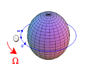
Figure 2: We consider the proper time difference (as measured by a clock rotating with constant angular velocity $\Omega$) between the emission and absorption of the co-propagating (+) and counter-propagating (-) beam.

The Sagnac effect has been thoroughly studied in the past, and it has been detected in many experiments (see [2] for a recent review). It is well known that when observing the interference between light or matter beams (such as light beams, electron or neutron beams and so on) counter-propagating in flat space-time along a closed path in a rotating interferometer a fringe shift $\Delta\Phi$ arises. This phase shift can be interpreted as a time difference between the propagation times (as measured by a clock at rest on the rotating interferometer) of the co-rotating and counter-rotating beam. In [1] we already showed that the Sagnac effect, for both matter and light beams, counter-propagating in a interferometer rotating in flat space-time, may be obtained by following a formal analogy with the Aharonov-Bohm effect: in a sense, it might be thought of as a gravito-magnetic Aharonov-Bohm effect. However, this procedure can be generalized to study the Sagnac effect in curved space-time, in order to obtain the General Relativistic corrections. In other words, we can study the interference process of matter or light beams in a rotating frame in curved space-time in terms of gravito-magnetic Aharonov-Bohm effect. This corresponds to calculating the phase shift (21) and the time difference (25) as measured, respectively, by a uniformly rotating interferometer and by an observer, provided with a standard clock. The time difference corresponds to the delay between the propagation time of the co-propagating and counter-propagating beam (see Figure 2). In what follows, the two beams are supposed to have the same velocity (in absolute value) with respect to the rotating frame.

For studying the Sagnac effect in stationary and axially symmetric geometries, it is sufficient to express the space-time metric in coordinates adapted to a congruence of rotating observers. Generally speaking the metrics we deal with are given in coordinates adapted to a congruence of asymptotically inertial observers; if the coordinates are spherical, the passage to a congruence of observers uniformly rotating in the equatorial plane is obtained by applying the (azimuthal) coordinate transformation:

$$\left\{\begin{array}[]{rcl}ct&=&ct^{\prime}\\ r&=&r^{\prime}\\ \varphi&=&\varphi^{\prime}-\Omega t^{\prime}\\ \vartheta&=&\vartheta^{\prime}\end{array}\right.\mathrm{\ .}$$ (26)

where $\Omega$ is the (constant) angular velocity.

Then, it is simple to apply the formalism that we have described so far. The following steps give a prescription for calculating the Sagnac effect in arbitrary stationary and axially symmetric geometries in both flat and curved space-times.

• Define the time-like congruence $\Gamma$ of rotating observsers
  

• Express the space-time metric in coordinates adapted to congruence of rotating observers

• Calculate the unit vectors field $\bm{\gamma}(x)$
  

  $$\left\{\begin{array}[]{l}\gamma^{{0}}=\frac{1}{\sqrt{-g_{{00}}}}\\ \gamma^{i}=0\end{array}\right.\;\;\;\;\;\;\;\;\;\;\;\;\left\{\begin{array}[]{l}\gamma_{0}=-\sqrt{-g_{{00}}}\\ \gamma_{i}=g_{i{0}}\gamma^{{0}}\end{array}\right.$$

• Calculate the gravito-electromagnetic potentials

  $$\left\{\begin{array}[]{c}\phi^{G}\doteq-c^{2}\gamma^{0}\\ \widetilde{A}_{i}^{G}\doteq c^{2}\frac{\gamma_{i}}{\gamma_{0}}\end{array}\right.$$

• Calculate the Sagnac time delay as a gravito-magnetic Aharonov-Bohm effect

  $$\Delta T=\frac{2\gamma_{0}}{c^{3}}\oint_{C}\widetilde{\bm{A}}_{G}\cdot{\rm d}\widetilde{\bm{x}}=\frac{2\gamma_{0}}{c^{3}}\int_{S}\bm{\widetilde{B}}_{G}\cdot{\rm d}\bm{\widetilde{S}}$$

  
  

  In the following, after reviewing the flat space-time case, we calculate the Sagnac effect in some curved space-times of physical interest. We consider beams counter propagating around the source of gravitational field, in its equatorial plane, along circular orbits of radius $R=constant$.

5.1 Minkowski space-time

The flat space-time metric, in cylindrical coordinates has the form:

$$ds^{2}=-c^{2}dt^{\prime 2}+dr^{\prime 2}+r^{\prime 2}d\varphi^{\prime 2}+dz^{\prime 2}$$ (27)

By performing an azimuthal transformation

$$\left\{\begin{array}[]{rcl}ct&=&ct^{\prime}\\ r&=&r^{\prime}\\ \varphi&=&\varphi^{\prime}-\Omega t^{\prime}\\ z&=&z^{\prime}\end{array}\right.\mathrm{\ .}$$ (28)

we get

$$ds^{2}=-\left(1-\frac{\Omega^{2}r^{2}}{c^{2}}\right)c^{2}dt^{2}+2\frac{\Omega r^{2}}{c}d\varphi cdt+dr^{2}+r^{2}d\varphi^{2}+dz^{2}$$ (29)

Then, the non null components of the vector field $\gamma$$(x)$, evaluated along the trajectories $r=R=constant$ are

$$\left\{\begin{array}[]{l}\gamma^{0}=\gamma\\ \gamma_{0}=-\gamma^{-1}\\ \gamma_{\varphi}=\frac{\gamma\Omega R^{2}}{c}\end{array}\right.$$ (30)

where $\gamma=\left(1-\frac{\Omega^{2}R^{2}}{c^{2}}\right)^{-\frac{1}{2}}$. As to the gravito-magnetic potential, we have

$$\widetilde{A}_{2}^{G}=\widetilde{A}_{\varphi}^{G}\doteq c^{2}\frac{\gamma_{\varphi}}{\gamma_{0}}=-\gamma^{2}\Omega R^{2}c$$ (31)

Consequently, the phase shift (21) becomes

$$\Delta\Phi=\frac{2m\gamma_{0}}{c\hbar}\int_{0}^{2\pi}\widetilde{A}_{\varphi}^{G}d\varphi=\frac{2m}{c\hbar\gamma}\int_{0}^{2\pi}\left(\gamma^{2}\Omega R^{2}c\right)d\varphi=4\pi\frac{m}{\hbar}\Omega R^{2}\gamma$$ (32)

and the proper time difference is

$$\Delta T=4\pi\frac{\Omega R^{2}\gamma}{c^{2}}\equiv\frac{4\pi R^{2}\Omega}{c^{2}}\left(1-\frac{\Omega^{2}R^{2}}{c^{2}}\right)^{-1/2}$$ (33)

Eq. (33) agrees with the well known Sagnac time delay (see for instance[15]).

5.2 Schwarzschild space-time

The standard form of the classical Schwarzschild solution, describing the vacuum space-time around a spherically symmetric mass distribution is

$$ds^{2}=-\left(1-\frac{2M}{r^{\prime}}\right)dt^{\prime 2}+\left(1-\frac{2M}{r^{\prime}}\right)^{-1}dr^{\prime 2}+r^{\prime 2}\left(d\vartheta^{\prime 2}+\sin^{2}\theta^{\prime}d\varphi^{\prime 2}\right)$$ (34)

where $M$ is the mass of the source, and the coordinate $(t,r,\vartheta,\varphi)$ are adapted to a congruence of asymptotically inertial observers. On applying the transformation (26) to (34), and setting $\vartheta=\frac{\pi}{2}$, we get

$$ds^{2}=-\left(1-\frac{2M}{r}-\Omega^{2}r^{2}\right)dt^{2}+\left(1-\frac{2M}{r}\right)^{-1}dr^{2}+r^{2}d\varphi^{2}+2\Omega r^{2}d\varphi dt$$ (35)

So, if we evaluate along the trajectories $r=R=constant$ the non null components of the vector field $\bm{\gamma}(x)$ relative to (35), we get

$$\left\{\begin{array}[]{l}\gamma^{0}=\gamma_{M}\\ \gamma_{0}=-\left(\gamma_{M}\right)^{-1}\\ \gamma_{\varphi}=\Omega R^{2}\gamma_{M}\end{array}\right.$$ (36)

and the only non null component of the gravito-magnetic potential turns out to be

$$\widetilde{A}^{G}_{\varphi}=-\Omega R^{2}\gamma^{2}_{M}$$ (37)

In both (36) and (37) we have introduced

$$\gamma_{M}\doteq\left(1-\frac{2M}{R}-\Omega^{2}R^{2}\right)^{-1/2}$$ (38)

Hence, the phase shift is given (in physical units) by

$$\Delta\Phi = \frac{2m\gamma_{0}}{c\hbar}\oint_{C}{\bf\widetilde{A}}^{G}\cdot{\rm d}\widetilde{\bm{r}}$$ (39)

$$= \frac{2m\gamma_{0}}{c\hbar}\int_{0}^{2\pi}\widetilde{A}_{\varphi}^{G}d\varphi$$

$$= \frac{4\pi m}{\hbar}\Omega R^{2}\gamma_{M}$$

while the corresponding time delay turns out to be

$$\Delta T=\frac{\hbar}{mc^{2}}\Delta\Phi=\frac{4\pi\Omega R^{2}}{c^{2}}\gamma_{M}$$ (40)

We see that if $\Omega=0$, i.e. if we measure the propagation time in a non rotating frame, no Sagnac effect arises. In other words, the propagation is symmetrical in both directions.

5.3 Kerr space-time

The Kerr solution [17] describes the space-time around a rotating black-hole or, more generally speaking, around a rotating singularity. The classical form of this solution is given in Boyer-Lindquist coordinates [18] $(t,r,\vartheta,\varphi)$, which are adapted to a congruence of asymptotically inertial observers:

$$ds^{2} = -(1-\frac{2Mr^{\prime}}{\rho^{2}})dt^{\prime 2}+\frac{\rho^{2}}{\Delta}dr^{\prime 2}+\rho^{2}d\vartheta^{\prime 2}+$$

$$+\left(r^{\prime 2}+a^{2}+\frac{2Mr^{\prime}a^{2}\sin^{2}\vartheta^{\prime}}{\rho^{2}}\right)\sin^{2}\vartheta^{\prime}d\varphi^{\prime 2}-\frac{4Mr^{\prime}a\sin^{2}\vartheta^{\prime}}{\rho^{2}}d\varphi^{\prime}dt^{\prime}$$

where $\rho^{2}=r^{\prime 2}+a^{2}\cos^{2}\vartheta^{\prime}$, and $\Delta=r^{\prime 2}-2Mr^{\prime}+a^{2}$, $a=J/Mc$, $J$ is the absolute value of the angular momentum, and the coordinates are arranged in such a way that the angular momentum is perpendicular to the equatorial plane.

By applying the transformation (26), and then setting $\vartheta=\frac{\pi}{2}$, we obtain

$$ds^{2} = -\left(1-\frac{2M}{r}+\frac{4Ma}{r}\Omega-(r^{2}+a^{2}+\frac{2Ma^{2}}{r})\Omega^{2}\right)dt^{2}+\frac{r^{2}}{\Delta}dr^{2}+r^{2}d\vartheta^{2}+$$ (42)

$$+\left(r^{2}+a^{2}+\frac{2Ma}{r}\right)d\varphi^{2}+\left(-\frac{2Ma}{r}+(r^{2}+a^{2}+\frac{2Ma}{r})\Omega\right)d\varphi dt$$

Consequently, we obtain the components of the vectors field of the congruence defining the rotating frame, evaluated along the trajectories $r=R=constant$:

$$\gamma^{0} = \gamma_{K}$$

$$\gamma_{0} = -(\gamma_{K})^{-1}$$

$$\gamma_{\varphi} = \left(-\frac{2Ma}{r}+(r^{2}+a^{2}+\frac{2Ma}{r})\Omega\right)\gamma_{K}$$ (43)

and the corresponding non null component of the gravito-magnetic potential is

$$\tilde{A}^{G}_{\varphi}=-c^{2}\left(-\frac{2Ma}{r}+(r^{2}+a^{2}+\frac{2Ma}{r})\Omega\right)\gamma^{2}_{K}$$ (44)

where in both (43) and (44) we introduced

$$\gamma_{K}\doteq\left(1-\frac{2M}{r}+\frac{4Ma}{r}\Omega-(r^{2}+a^{2}+\frac{2Ma^{2}}{r})\Omega^{2}\right)^{-1/2}$$ (45)

Consequently, the phase shift turns out to be (in physical units)

$$\Delta\Phi = \frac{2m\gamma_{0}}{c\hbar}\oint_{C}{\bf\widetilde{A}}^{G}\cdot{\rm d}\widetilde{\bm{r}}$$ (46)

$$= \frac{2m\gamma_{0}}{c\hbar}\int_{0}^{2\pi}\widetilde{A}_{\varphi}^{G}d\varphi$$

$$= \frac{4\pi mc}{\hbar}\left(-\frac{2GMa}{c^{2}R}+(R^{2}+a^{2}+\frac{2GMa}{c^{2}R})\frac{\Omega}{c}\right)\gamma_{K}$$

and the corresponding time delay is

$$\Delta T=\frac{\hbar}{mc^{2}}\Delta\Phi=\frac{4\pi}{c}\left(-\frac{2GMa}{c^{2}R}+(R^{2}+a^{2}+\frac{2GMa}{c^{2}R})\frac{\Omega}{c}\right)\gamma_{K}$$ (47)

By explicitly writing $\gamma_{K}$ we get

$$\Delta T=\frac{4\pi}{c}\frac{\left(-\frac{2GMa}{c^{2}R}+(R^{2}+a^{2}+\frac{2GMa}{c^{2}R})\frac{\Omega}{c}\right)}{\left(1-\frac{2GM}{c^{2}R}+\frac{4GMa}{c^{2}R}\frac{\Omega}{c}-(R^{2}+a^{2}+\frac{2GMa^{2}}{c^{2}R})\frac{\Omega^{2}}{c^{2}}\right)^{1/2}}$$ (48)

The time delay (48) is in agreement with the results obtained by Tartaglia [4], who studied in full details the General Relativistic corrections to the Sagnac effect in Kerr space-time. Tartaglia also evaluated the approximations of the time delay (48). In the following Subsection we shall obtain approximated results for the General Relativistic corrections to the Sagnac effect by starting from the weak field solution of Einstein equations around a rotating mass.

5.4 The weak field around a rotating mass

The space-time around a weakly gravitating object of mass $M$ and angular momentum $\bm{\vec{J}}$ is given by

$$ds^{2} = -\left(1-\frac{2M}{r^{\prime}}\right)dt^{\prime 2}+\left(1+\frac{2M}{r^{\prime}}\right)\left[dr^{\prime 2}+r^{\prime 2}\left(d\vartheta^{\prime 2}+\sin^{2}\vartheta^{\prime}d\varphi^{\prime 2}\right)\right]+$$ (49)

$$-\frac{4J}{r^{\prime}}\sin^{2}\vartheta^{\prime}d\varphi^{\prime}dt^{\prime}$$

where the spherical coordinates $(t,r,\vartheta,\varphi$) (adapted to a congruence of a asymptotically inertial observers) have been arranged in such a way that the angular momentum is orthogonal to the equatorial plane.

If we apply to the metric (49) the transformation (26), after setting $\vartheta=~{}\frac{\pi}{2}$, we obtain

$$ds^{2} = -\left[1-\frac{2M}{r}-\left(1+\frac{2M}{r}\right)\Omega^{2}r^{2}+\frac{4J\Omega}{r}\right]dt^{2}+$$

$$+\left(1+\frac{2M}{r}\right)\left[dr^{2}+r^{2}d\varphi^{2}\right]+2\left[\left(1+\frac{2M}{r}\right)\Omega r^{2}-\frac{2J}{r}\right]d\varphi dt$$

Then, the non null components of the vector field $\bm{\gamma}(x)$, along the trajectories $r=R=constant$, are

$$\gamma^{0} = \gamma_{J}$$

$$\gamma_{0} = -(\gamma_{J})^{-1}$$

$$\gamma_{\varphi} = \left[\left(1+\frac{2M}{R}\right)\Omega R^{2}-\frac{2J}{R}\right]\gamma_{J}$$ (51)

and the corresponding component of the gravito-magnetic potential is

$$\widetilde{A}^{G}_{\varphi}=-\left[\left(1+\frac{2M}{R}\right)\Omega R^{2}-\frac{2J}{R}\right]\gamma^{2}_{J}$$ (52)

In both (51) and (52) we have introduced

$$\gamma_{J}\doteq\left[1-\frac{2M}{R}-\left(1+\frac{2M}{R}\right)\Omega^{2}R^{2}+\frac{4J\Omega}{R}\right]^{-1/2}$$ (53)

As a consequence, re-introducing physical units, we have

$$\Delta\Phi = \frac{2m\gamma_{0}}{c\hbar}\oint_{C}{\bf\widetilde{A}}^{G}\cdot{\rm d}\widetilde{\bm{r}}$$ (54)

$$= \frac{2m\gamma_{0}}{c\hbar}\int_{0}^{2\pi}\widetilde{A}_{\varphi}^{G}d\varphi$$

$$= \frac{4\pi m}{\hbar}\left[\left(1+\frac{2GM}{c^{2}R}\right)\Omega R^{2}-\frac{2GJ}{c^{2}R}\right]\gamma_{J}$$

and the corresponding time delay is

$$\Delta T=\frac{\hbar}{mc^{2}}\Delta\Phi=\frac{4\pi}{c^{2}}\left[\left(1+\frac{2GM}{c^{2}R}\right)\Omega R^{2}-\frac{2GJ}{c^{2}R}\right]\gamma_{J}$$ (55)

or, by explicitly writing $\gamma_{J}$

$$\Delta T=\frac{4\pi}{c^{2}}\frac{\left[\left(1+\frac{2GM}{c^{2}R}\right)\Omega R^{2}-\frac{2GJ}{c^{2}R}\right]}{\left[1-\frac{2GM}{c^{2}R}-\left(1+\frac{2GM}{c^{2}R}\right)\frac{\Omega^{2}R^{2}}{c^{2}}+\frac{4GJ\Omega}{c^{2}R}\right]^{1/2}}$$ (56)

In (54) and (55) we can distinguish two contributions: the first one is proportional to the angular velocity $\Omega$ of the observer, and the other one depends on the absolute value of the angular momentum of the source $J$.

We see that even when $\Omega=0$ a time difference appears: this is due to the rotation of the source of the gravitational field (the same holds in Kerr space-time). In other words

$$\Delta T_{J}\doteq\frac{4\pi}{c^{2}}\frac{\left[-\frac{2GJ}{c^{2}R}\right]}{\left[1-\frac{2GM}{c^{2}R}\right]^{1/2}}$$ (57)

is what an asymptotically inertial observer would obtain when measuring the propagation time for a complete round trip of the two beams, moving in opposite direction along circular orbits $r=R=constant$. This time difference corresponds to the so called gravito-magnetic time delay, which has been obtained by Stodolski[19], Cohen-Mashhoon[5] in weak field approximation, and by Tartaglia, by a first order approximation of the time delay in Kerr space-time.

6 Conclusions

In the context of natural splitting, the relative formulation of dynamics can be expressed in terms of gravito-electromagnetic fields; this analogy, which holds in full theory, leads to the formulation of the gravito-magnetic Aharonov-Bohm effect. We showed that the Sagnac effect can be interpreted as a gravito-magnetic Aharonov-Bohm effect in both flat and curved space-time, and we exploited this formal analogy for calculating the General Relativistic corrections to the Sagnac effect, in stationary and axially symmetric geometries. The results that we obtained, are in agreement with those available in the literature, and generalize some old approaches.

The Sagnac effect has a ”universal” character: in other words, the Sagnac time delay is the same, independently of the physical nature and velocities of the interfering beams, provided that the latter are the same, in absolute value, as seen in the rotating frame. In our formalism this universality is expressed by Eq. (25), where the mass (or the energy) of the particles of the beams does not appear, and it is explained as an effect of the geometrical background in which the beams propagate. Hence, the geometrical approach clearly points out the universal character of the effect.

References

- [1] Rizzi G., Ruggiero M.L., Gen. Rel. Grav. 35, 1743 (2003), gr-qc/0305046
- [2] Rizzi G., Ruggiero M.L., in Relativity in Rotating Frames, eds. Rizzi G. and Ruggiero M.L., in the series “Fundamental Theories of Physics”, ed. A. Van der Merwe, Kluwer Academic Publishers, Dordrecht (2004), gr-qc/0305084
- [3] Sakurai J.J., Phys. Rev. D 21, 2993 (1980 )
- [4] Tartaglia A., Phys. Rev. D 58, 064009 (1998)
- [5] Cohen J.M., Mashhoon B., Phys. Lett. A 181, 353 (1993)
- [6] Ferrarese G., Lezioni di Relatività Generale, Pitagora Editrice, Bologna (2001)
- [7] Mashhoon B., Gronwald F., Lichtenegger H.I.M., Lect. Notes Phys. 562, 83 (2001), gr-qc/9912027
- [8] Ruggiero M.L., Tartaglia A., Il Nuovo Cimento B 117, 743 (2002), gr-qc/0207065
- [9] Mashhoon B., (2003), gr-qc/0311030
- [10] Aharonov Y. and Bohm D., Phys. Rev. 115, 485 (1959)
- [11] Tourrenc P., Phys. Rev. D 16, 3421 (1977)
- [12] Hehl F.W. and Ni W.T., Phys. Rev. D 42, 2045 (1990)
- [13] Mashhoon B., Phys. Rev. Lett. 61, 2639 (1988)
- [14] Papini G., in Relativity in Rotating Frames, ed. Rizzi G. and Ruggiero M.L., in the series “Fundamental Theories of Physics”, ed. A. Van der Merwe, Kluwer Academic Publishers, Dordrecht (2004)
- [15] Rizzi G., Ruggiero M.L., Gen. Rel. Grav. 35, 2129 (2003), gr-qc/0306128
- [16] Misner C.W., Thorne K.S., Wheeler J.A., Gravitation, Freeman, S.Francisco (1973)
- [17] Kerr R.P. , Phys. Rev. Lett 11, 237 (1963)
- [18] Boyer R.H., Lindquist R.W., J. Math. Phys 8, 265 (1967)
- [19] Stodolsky L., Gen. Rel. Grav. 11, 391 (1979)