Abstract
We study the correction to the scale invariant power spectrum of a scalar field on de Sitter space from small black holes that formed during a pre-inflationary matter dominated era. The formation probability of such black holes is estimated from primordial Gaussian density fluctuations. We determine the correction to the spectrum of scalar cosmological perturbations from the Keldysh propagator of a massless scalar field on Schwarzschild-de Sitter space. Our results suggest that the effect is strong enough to be tested – and possibly even ruled out – by observations.
ITP-UU-10/23
SPIN-10/20
Scalar cosmological perturbations
from inflationary black holes
Tomislav Prokopec111email: t.prokopec@uu.nl and Paul Reska222email: p.m.reska@uu.nl
Spinoza Institute and Institute for Theoretical Physics
Utrecht University
Leuvenlaan 4, 3584 CE Utrecht, The Netherlands
Keywords: primordial black holes, inhomogeneous cosmology, cosmological perturbations, slow-roll inflation
1 Introduction
Measurements of the cosmic microwave background (CMB) show that the Universe is isotropic on large scales to very good precision. Indeed, the CMB radiation is an almost perfect black body [1] with a temperature of [2], and tiny temperature fluctuations superimposed with an amplitude of the order [3]. The exception is the dipole, which is at the level of , and can be explained by our motion with respect to the CMB rest frame. The assumption that measurements at any position in the Universe would lead to the same result implies that the Universe is also homogeneous. Observations of large scale structure support this assumption [4]. This Einstein’s Cosmological Principle is a corner stone of modern cosmology and, hence, it is important to further experimentally test its validity.
There has been much interest recently in the possibility that small violations of homogeneity and/or isotropy could give rise to the observed CMB anomalies. Some of the often quoted CMB anomalies are [5, 6]: an anomalously small quadrupole and octupole moments; a large deviation from the mean in some of the higher multipoles; the north-south asymmetry, the peculiar alignment of the quadrupole and octupole and their pointing in the direction of Virgo [7]; the alignment of some of the higher multipoles [8]; the curious lack of power in the temperature angular correlation function on large angular scales [5], etc. Different authors disagree however in what constitutes significant deviation from homogeneity and isotropy. For example, Bennett et al. [5] tend to tune down the statistical significance of these anomalies, and argue that most of them can be attributed to priors. They also argue that, in the absence of a deep theoretical justification, which would make further tests possible, these anomalies will most likely remain curiosities. In addition to the CMB anomalies, there are also anomalies in the large scale structure of the Universe. For example, observational evidence was reported by Kashlinsky and collaborators [12] for large scale (dark) flows of galactic clusters which cannot be explained by homogeneous, adiabatic, Gaussian, cosmological perturbations generated during inflation. Moreover, some authors [9, 10] offer an alternative to dark energy by considering the earth to be located near the center of a large void [10], or by considering a randomly distributed collection of voids in the Universe (the Swiss cheese Universe) [11].
The question we pose in this paper is whether some of these anomalies can be explained by placing a small black hole into an inflationary universe. 333Our study of small black holes can be quite easily extended to point-like particles such as magnetic monopoles or heavy particles whose mass is of the order the Planck mass. However, we expect that the effect of these particle-like objects will in general be much smaller than that of primordial black holes, giving thus a competitive edge to the study of black holes in inflation. Since answering this question rigorously is hard, here we make a first step in addressing it. In order to model cosmological perturbations we consider quantum fluctuations of a massless (or light) scalar field minimally coupled to gravity in Schwarzschild-de Sitter (SdS) space, and calculate the corresponding spectrum. Based on the knowledge of the Mukhanov-Sasaki gauge invariant potential, we then estimate the spectrum of scalar cosmological perturbations. We make the assumption that the gauge invariant treatment also applies to the inhomogeneous cosmology at hand, but warn the reader that our approach should be tested by a rigorous study of cosmological perturbations in inhomogeneous settings such as inflation endowed with a small black hole. In this paper we ignore tensor perturbations, since we expect that their amplitude will be, just as in homogeneous cosmologies, suppressed when compared to that of scalar perturbations. Furthermore, the effect of vector modes is not taken into account because they are not dynamical for a homogeneous background and hence we expect them to play a subdominant role in the case of weak breaking of homogeneity that we consider.
It is an important question how to relate our results for the primordial spectrum of scalar cosmological perturbations to the CMB observables. An interesting study in this direction is Ref. [13], where the authors investigate how different types of violation of homogeneity and isotropy would affect the temperature fluctuations in the CMB. Based on symmetry considerations, the authors consider in particular how a point-like defect (particle), a line-like defect (cosmic string) or a plane-like defect (domain wall) would modify the observed temperature anisotropies. By symmetry a small black hole is closest to a point-like object, yet its event horizon makes it a more complex object to study. 444A further complication is in the fact that a black hole could rotate and/or move with respect to the inflaton’s rest frame. The latter could in principle be related to the claimed large scale dark flows [12]. While the analysis in [13] is useful to make a connection between cosmological perturbations generated in inflation and temperature fluctuations, it is not general enough to suit our needs. In particular, it cannot be used for a primordial black hole whose comoving distance from us is small in comparison to the wavelength of the perturbation considered.
The main theoretical motivation for studying spectral inhomogeneities generated by a stationary black hole in inflation is that they yield results that can be tested against observations. This is so because the resulting spectrum can be viewed as a six parameter template. A good analogue are the gravitational wave templates provided by black hole binary systems. To illustrate more precisely what we mean, recall that homogeneous inflation produces a (power law) spectrum which, as a function of spatial momentum , can be viewed as a two-parameter template, the parameters being the spectral amplitude () and its slope (), which have been by now tightly constrained by CMB measurements [14]. When viewed as a template, the SdS spectrum contains four additional parameters. These constitute the black hole position with respect to us and its mass during inflation 555Of course, the black hole has by now evaporated., which we parametrize by . Here denotes the de Sitter Hubble parameter, and is Newton’s constant. 666If in addition the black hole is moving, three additional parameters are needed to specify its velocity; if it is rotating, three additional parameters are needed to specify its angular momentum; if it is charged, one more parameter is needed. We shall not study here observational consequences of these more general settings. Regarding the results presented in Ref. [12], it would be of particular interest to study the spectrum of a (slowly) moving black hole. In the light of the upcoming CMB observatories, such as the Planck satellite, and ever increasing large scale galactic redshift surveys, it is clear that we will be able to test the inflationary black hole hypothesis.
The paper is organized as follows. In section 2 we present the inhomogeneous Schwarzschild-de Sitter background metric and the corresponding scalar field equation of motion. We make a simple estimate of the number of black holes per Hubble volume at the beginning of inflation in section 3. Then, in section 4 we derive a formula which relates the amplitude of inflaton fluctuations on Schwarzschild-de Sitter space to the spectrum of scalar cosmological perturbations. The Schwinger-Keldysh propagator is derived in section 5 by expanding in the parameter . Section 6 deals with the application to cosmology. In particular, we obtain the power spectrum and illustrate its features in various plots in section 7. We close our paper in section 8 with a discussion. Various technical details are relegated to four appendices. In this paper we work in units where , but we keep Newton’s constant , the reduced Planck mass, and the Planck mass .
2 Inflaton field on Schwarzschild-de Sitter space
2.1 Background metric and equation of motion
A primordial black hole breaks the translational invariance of the background but does preserve rotational symmetry. The space-time metric of a black hole in an asymptotically homogeneous universe is the Schwarzschild-de Sitter (SdS) solution, giving rise to a line element which is usually written in static coordinates as
| (1) |
with . In these coordinates the three symmetries of the SdS space are manifest: the time translation invariance and the two spatial rotations. Quantum fluctuations of a scalar field on the Schwarzschild background have been dealt with in Ref. [15], where it was found that the radial mode functions of a massless scalar field can be expressed in terms of Heun’s functions. But the presence of a cosmological horizon complicates the analysis and the SdS case has only been discussed for an extremal black hole [16]. The reason for this is the difficult singularity structure of the d’Alembertian for (1). For applications to cosmology another form of the metric is more useful. In Appendix A we show by explicit coordinate transformations that the metric takes the form 777A similar form of the metric can be found in [17]. However, it has the disadvantage of being degenerate at the black hole horizon.
| (2) |
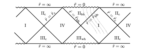
with and the scale factor which is a simple function of conformal time , (). Notice that the metric (2) exhibits a black hole singularity at a finite radius, (see also Eq. (110)), such that in this metric covers one half of SdS space. The Carter-Penrose diagram is plotted in Fig. 1 (see also [18]) which also shows (schematically) how the interior of the black hole is covered by our coordinates.
The Hubble rate is related to the potential energy of the inflaton through the Friedmann equation, . Here we assume that the inflaton potential energy is constant, such that it can be related to the effective cosmological constant as .
The equation of motion for the massless inflaton field is the Klein-Gordon equation,
| (3) |
where the d’Alembertian acting on a scalar field is given by
| (4) |
One easily finds from the determinant of the metric tensor,
| (5) |
and hence
| (6) | ||||
where is the Laplacian on the 2-dimensional sphere,
Because the CMB is highly isotropic, translation invariance in the early Universe can be only weakly broken [5, 6]. Hence and we can expand the metric in the parameter to first non-trivial order. The result is:
| (7) | ||||
The differential operator is the d’Alembertian on de Sitter space,
| (8) |
and
| (9) |
with and is the Cartesian Laplace operator in 3 dimensions.
2.2 An estimate of the perturbation parameter
The metric (2) contains the perturbation parameter as a constant. A more realistic point of view, however, is that a black hole of mass decays due to an evaporation process and is a time-dependent expansion rate of the Universe. Assuming a slow-roll inflationary scenario, i.e. small deceleration parameter
| (10) |
we can neglect the time-dependence of in the following discussion. Further comments on this approximation are made in section 4. For the rate of change of we make the following estimate. The evaporation time of a black hole is known to be [19, 20]
| (11) |
where is the number of relativistic degrees of freedom at the energy scale . The correction to the evaporation time (11) due to the Hubble horizon is negligible as long as [20]. Assuming that the evaporation process takes longer than e-foldings, we get
| (12) |
where we took and . In summary, for primordial black holes with a mass parameter we expect the SdS background to be a good realization of the inhomogeneous inflationary scenario. The constancy of is demonstrated in Fig. 2.

3 Formation probability for black holes
To assess the physical relevance of primordial black holes, we first estimate the probability for their formation. For this we consider a pre-inflationary period dominated by heavy non-relativistic particles with a mass and Hubble rate (here and henceforth an index refers to quantities evaluated at the initial time ). The presence of such particles is generally expected in physics at the GUT scale [21]. Moreover, such a scenario has recently been discussed in connection with CMB anomalies [22, 23]. On not too small scales the matter distribution in this pre-inflationary phase is well described by the local mass density . For black hole formation we are interested in the growth of density fluctuations inside of a bounded region. The number of particles in a comoving ball with physical radius and volume at time is denoted by . The initial statistical fluctuations for the particle number are assumed to be Gaussian, with variance . The mass density in the ball is linearly related to the local density,
| (13) |
which can also be written as . Fluctuations in the particle number are thereby easily translated into density fluctuations.
Black holes can potentially form from gravitational interaction of such fluctuations [19]. Due to the attractive nature of gravity, fluctuations can grow. To study their evolution, we consider the classical equation of motion for : 888cf. Bonometto (ed.), ‘Modern Cosmology’ (2002), p. 50.
| (14) |
with the speed of sound , where is the background fluid pressure. We take the equation of state parameter to be constant. The Universe is assumed to be dominated by one species of particles in which case one can neglect entropy fluctuations, , which would otherwise appear on the right hand side of Eq. (14). When the gravitational term dominates in the above equation the density perturbation becomes unstable. The critical scale for the perturbation is given by the Jeans momentum
| (15) |
which determines when thermal pressure is in balance with the gravitational force. The Jeans length reaches the Hubble scale if . For the Jeans length is very small compared to the Hubble radius and small black holes can form. We can solve Eq. (14) for (super-Jeans scale) by making the Ansatz and we find that
| (16) |
We shall neglect the second mode which is always decaying. In decelerating space-times () the first mode is growing, whereas in accelerating space-times () fluctuations always decay due to the repulsive nature of gravity. The amplification actually increases with increasing but, as mentioned before, we are only interested in the case since in this case , which also has to be satisfied for the growing solution. The initial density perturbation is given by
| (17) |
Clearly, we have to look at large fluctuations away from the mean value to find a significant probability of black hole formation. It is convenient to translate momentum space fluctuations to fluctuations in a ball of radius by writing
| (18) |
with being the angle averaged momentum space mass density and
| (19) |
is the well-known window function for spherically distributed matter in a ball of radius . From relation (18) we conclude that grows precisely as the momentum space fluctuations (16),
| (20) |
Next, note that
| (21) |
which follows from the Friedmann equation, and from
Now from Eq. (17) and (21) we can write,
| (22) |
and hence
| (23) |
Due to the expansion of the Universe, the radius of the ball grows as in (23). In a decelerating universe, , the comoving radius grows slower than the Hubble radius, , such that, if initially at , it will remain sub-Hubble at later times. This trend reverses during inflation, in which .
A black hole with Schwarzschild radius forms if, due to statistical fluctuations, the number of particles in becomes sufficiently large, , . Using (21) and writing one obtains the condition
| (24) |
Thus, using that the fluctuations are Gaussian distributed 999Recall that, from the central limit theorem, the Gaussian distribution is the large limit of the Poisson distribution.,
with , the probability that a black hole forms is found to be 101010In the limit the statistical fluctuations could also obey a power law behavior, , like in the theory of critical phenomena. We are not going to consider this possibility here in any detail. Note, however, that for this type of statistical fluctuations more black holes will form.
| (25) |
where, making use of Eqs. (23) and (24),
| (26) |
The inequality in (26) is needed to correctly evaluate the integral (25). Notice also that, when that inequality is met, the probability for black hole formation is (exponentially) suppressed. Clearly, the inequality is broken for super-Hubble scales, for which . But at super-Hubble scales we expect suppressed statistical fluctuations, and hence do not trust our analysis anyway (see the comment further below). Remarkably, up to the term, Eq. (26) is time independent, which also means that the probability for black hole formation (25) in a ball of constant comoving radius is time independent. Hence, the growth of perturbations (20) precisely compensates the decay in fluctuations (17). This might be telling us something deep about gravity. However, we do not have a simple explanation for this fact. For later purposes it is useful to rewrite our result for the probability of black hole formation (25–26) as
| (27) |
where we made use of the mass parameter . Obviously, must be satisfied in order for a black hole to be sub-Hubble. The question is then how to convert the probability (25) into the number of black holes formed before inflation and during inflation. The analysis presented above is meant to provide a rough estimate of the number of sub-Hubble black holes formed before inflation, and neither takes a proper account of causality, nor of nonlinear dynamics of over-densities. Staying within this type of reasoning, we propose to interpret (27) as an estimate for the probability that a black hole formed by the beginning of inflation in a comoving volume . The expected number of black holes per Hubble volume at the beginning of inflation is then
| (28) |
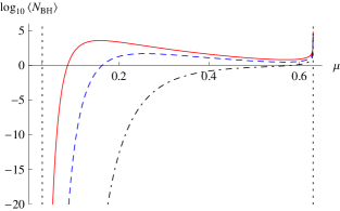
If the Hubble volume today corresponds to Hubble volumes at the beginning of inflation, then there will be about pre-inflationary black holes within our past lightcone. A more detailed discussion on how to relate the number of black holes (28) to the number of (pre-)inflationary black holes potentially observable today is given in section 8. In Fig. 3 we show how the expected number of black holes (28) depends on the black hole mass parameter for different values of particle mass and initial Hubble rate . We emphasize, however, that in our analysis we make the assumption that the statistical fluctuations are normally distributed on all scales. This might not be true, as has been argued for example in [24], where fluctuations of other types are considered on super-Hubble scales. Causality can limit the size of these statistical fluctuations. It may be more realistic to assume that on super-Hubble scales surface fluctuations are dominant, and , thus, suppressing the formation of black holes that are initially super-Hubble. The actual probability for black hole formation might therefore be smaller in the region than it is shown in Fig. 3. Moreover, the formation probability depends strongly on the mass of the heavy particles, and yet we do not know much about it. Based on our current understanding of particle physics and gravity, it is reasonable to assume that is limited from above by the Planck mass . If , however, the particles would start behaving relativistically, which would increase the Jeans length and further suppress, or even prevent, the formation of black holes.
4 From scalar fluctuations to scalar cosmological perturbations
4.1 Homogeneous background
Before discussing the effect of inhomogeneities on the scalar spectrum, we review the treatment of cosmological perturbations on homogeneous backgrounds, such as the conformally flat background metric, , where and is the scale factor of the Universe. The physical situation we have in mind is a slow-roll inflationary model driven by a homogeneous inflaton field , where the Hubble parameter () is a slowly varying function of time, such that the de Sitter limit is obtained when Scalar perturbations in this model are induced by the quantum fluctuations of the inflaton, while tensor perturbations are induced by the quantum fluctuations of the graviton. In linearized perturbation theory the two decouple. For a recent treatment we refer to [25], while standard reviews are Refs. [26, 27].
It is convenient to decompose the inflaton and the metric tensor into the background fields and the fluctuations as follows,
The background fields and are classical field configurations, whereas and are dynamical quantum fields. A detailed study (see e.g. [25]) shows that there are only three physical degrees of freedom, two from the graviton and one from the scalar field. These can be expressed in terms of the gauge invariant Mukhanov-Sasaki variable (), and the gauge invariant tensor , where by gauge invariance we mean the invariance under linear coordinate shifts . Since physical observables are independent of the choice of gauge, it is convenient to work with gauge invariant fields. In homogeneous cosmology the Sasaki-Mukhanov field (curvature perturbation) is of the form,
| (29) |
where is the scalar gravitational potential defined by the scalar-vector-tensor decomposition of :
| (30) |
and is the inflaton fluctuation. The potential is a gauge variant measure for local spatial volume fluctuations. When working with gauge invariant variables, such as in (29), we are guaranteed to get observable CMB temperature fluctuations, since it is the gradient of that sources photon number fluctuations through the photon Boltzmann equation. One can also get a physically sensible answer when one fixes a gauge, provided one makes the correct link to the late time gravitational potential which enters the fluid equations.
For example, in the comoving gauge, in which , it is the spatial gravitational potential that determines the Sasaki-Mukhanov field, (29). On the other hand, in the zero curvature gauge, in which , it is the inflaton fluctuation that determines through (29),
| (31) |
This relation can be used to estimate the late time potential from the inflaton fluctuations . The spectrum of scalar cosmological perturbations in zero curvature gauge, ( is conserved on super-Hubble scales) is related to the spectrum of scalar field fluctuations as,
| (32) |
where denotes the reduced Planck mass. In order to get the latter identity, we used the second Friedmann equation, , and the definition for the slow-roll parameter, .
Of course, there are two remaining degrees of freedom in the graviton which have not been taken into account. However, the graviton spectrum is known to be suppressed in the slow-roll inflation [28, 14, 25]
| (33) |
such that, to first approximation, we can neglect the graviton contribution to the spectrum of cosmological perturbations.
Finally, the field fluctuations can be translated to the temperature-temperature correlation function as [13],
where denotes a Legendre polynomial, and and denote the appropriate transfer functions, which relate to , and which are obtained by solving the Boltzmann equation for the photon fluid.
4.2 A small black hole in a de Sitter Universe
Keeping in mind the procedure of the previous section for the derivation of cosmological perturbations from scalar fluctuations, we have to pay special attention to use gauge invariant fields also in the inhomogeneous case. We split the metric into the Schwarzschild-de Sitter background (7) and a perturbation . The spatial part of the perturbation can be decomposed as
| (35) |
where is the induced metric on the spatial slices for the metric (7) and is the covariant derivative compatible with . The vector that generates the gauge transformation can be written as , with and . The metric perturbation transforms as
| (36) | ||||
with the Christoffel symbols of the metric (7)
| (37) |
and with
| (38) |
Moreover, we observe that is traceless to the relevant order in , showing that generates also transformations of and . The transformation properties of the two scalars and are
| (39) |
Together with the gauge transformation of the scalar field, , we find that
| (40) |
We conclude that the Sasaki-Mukhanov field in Eq. (29) is gauge invariant (to order ) also when the inhomogeneity caused by a small black hole is taken into account.
The fact that generates gauge transformations of a vector and the tensor suggests a mixing of the scalar, vector and tensor sectors in inhomogeneous cosmology. Therefore, for a completely rigorous treatment one should look at the quadratic action on the SdS background and take into account the couplings of the modes.
Furthermore, we make use of the slow-roll paradigm. This means that, even though strictly speaking our results will be derived in SdS space, we shall assume that they hold in quasi de Sitter space endowed with a small (decaying) black hole, provided one exacts the replacements: and . This is justified when both the Hubble parameter and the black hole mass change adiabatically in time, in the sense that () and .
5 The propagators
To study scattering experiments, one typically calculates the S-matrix elements. In cosmology, on the other hand, one is primarily interested in expectation values of operators with respect to some definite vacuum state. For this purpose the in-in, or Schwinger-Keldysh [29, 30], formalism [31, 32, 25] is suitable, in which time evolution of an operator is described in terms of the perturbation theory based on the Keldysh propagator and the in-in vertices. Since here we are primarily interested in the spectrum of a scalar field on SdS space, which can be obtained from any equal time two-point correlator, for our purpose it suffices to calculate the corresponding Keldysh propagator.
The Keldysh propagator is a -matrix of the form,
| (43) |
whose components are the Wightman functions , and (anti-)time ordered Feynman propagators , , defined as,
| (44) | |||||
where is a suitably chosen vacuum state. The time ordering is defined as
| (45) | ||||
i.e. later times are to the left for and early times are to the left for . The propagator satisfies the equation
| (46) |
where is the Pauli matrix
| (47) |
and is the effective mass-squared of the field, which in the following we neglect. In slow-roll inflation can be expressed in terms of the second slow-roll parameter , i.e. , such that setting is equivalent to .
5.1 The de Sitter case
In the de Sitter case we can solve the equation of motion for the massless scalar field (3–4) explicitly. Taking advantage of spatial homogeneity of de Sitter space, the following mode decomposition of the free field is convenient,
| (48) |
where and are the annihilation and creation operators, defined by and by the commutation relation, . The mode functions in (48) satisfy the equation
| (49) |
We obtained this result by making use of (8) and noting that implies . Imposing the boundary condition that the mode functions behave like in the conformal vacuum in the asymptotic past yields
| (50) |
This equation, together with the condition (for all ), defines the Bunch-Davies (BD) vacuum . The fact that in the ultraviolet () the BD vacuum minimizes the energy in the field fluctuations has led to the belief that this vacuum represents a sensible physical choice [33] for the inflationary vacuum. This is not so because in the infrared (where ) the BD vacuum yields infinite energy. Namely, in the IR adiabaticity of the state is broken because the field couples strongly to the expanding background, leading to abundant particle generation, having as a consequence strongly enhanced infrared correlations. While this particle creation is very welcome in cosmology, since the amplified vacuum fluctuations provide a beautiful explanation for the Universe’s structure formation, one has to take proper care to regulate the IR. One way of doing that is to replace the BD vacuum by a more general state, characterized by the following generalization of the mode functions (50),
| (51) |
By suitably choosing , one can then make the infrared part of the vacuum state finite [34]. A concrete working realization of this proposal has been investigated in Refs. [35, 36]. Alternatively, one can remove the infrared problems by placing the Universe in a large comoving box of size . This leads to a discretized reciprocal (momentum) space [, with integers], with the comoving lattice size . Since corresponds to the minimum allowed momentum, this cures the infrared problem simply by disallowing the deeply infrared modes. In the limit when , the lattice constant , and the sum over the momenta can be replaced with increasing accuracy by an integral, which has as the IR cut-off, thus regulating the infrared. From the physical point of view, it is natural to associate this cut-off with the scale of the Hubble horizon at the beginning of inflation, thereby eliminating modes that stretch beyond the Hubble radius. One way of implementing this, is to take the spatial topology of the universe to be compact, e.g. a torus, as discussed in [37].
To see how the regularization procedure works in practice, we shall now calculate the regulated Feynman propagator in de Sitter space. In order to do that, we need to relate the direct space propagator to its mode functions (50). Because de Sitter space is spatially homogeneous, it is convenient to write the components of the Keldysh propagator (43) for de Sitter space in terms of its Fourier space counterparts,
| (52) |
Making use of Eqs. (48) and (50), one finds for the momentum space propagators,
| (53) | |||
The corresponding spectrum , defined by
| (54) |
is obtained straightforwardly from the equal time limit () of the propagator,
| (55) |
It is scale invariant at future infinity, .
Based on (53) one can calculate the position space de Sitter propagator by performing the momentum integral (52) over . The resulting Feynman propagator is [38, 39],
| (56) |
where is the conformal space distance function. Two comments are in order. Firstly, apart from the standard Hadamard contribution , which is singular on the lightcone (on-shell) and quickly decays off-shell, due to rapid particle production in de Sitter space, the de Sitter propagator (56) acquires a logarithmic term which contributes both within the past and future light cones. Secondly, the logarithm grows without a limit as . This is a manifestation of the IR singularity of the Bunch-Davies vacuum. We will see below that a black hole in de Sitter space ‘sees’ this logarithmic singularity in the corrected SdS propagator as a logarithmic singularity in the mixed space propagator and hence also in the (mixed space) SdS spectrum. This dependence on the IR regulator poses a unique opportunity to investigate the black hole contribution to the spectrum dependent on the IR regularization. In this paper we choose the comoving box regulator primarily because of its simple implementation, but one would certainly benefit from studying other IR regularization schemes.
5.2 The Schwarzschild-de Sitter case
For the case when a primordial black hole is present in de Sitter space we shall derive only the first order correction in to the Schwinger-Keldysh propagator. For this we write
| (57) |
with being the propagator on de Sitter space (52–53), (56). By plugging this into (46) we find that the correction to satisfies:
| (58) | ||||
Note that is only , and we will neglect it from now on. It follows that
| (59) |
This solution of (58) is given only up to a homogeneous solution of the d’Alembertian operator in (58). The unique propagator in (59) is obtained upon specifying the boundary conditions for the mode functions, or equivalently, for the vacuum state. Here the unperturbed vacuum state is chosen to be the (pure) Bunch-Davies vacuum of de Sitter space, whereby the deep infrared modes are removed by placing the Universe in a comoving box, as explained in section 5.1. But we are still free to add a homogeneous solution to the Feynman propagator (resulting in a mixed state), which has to be added to take Hawking radiation into account. The light black holes that we consider do indeed emit Hawking radiation but a simple estimate 111111From Table 1 in [15] one can in principle obtain an explicit expression for the asymptotic form of the (renormalized) propagator for Hawking radiation in the Unruh vacuum, which is the physically relevant state in this case. However, a rigorous treatment of the effect of Hawking radiation requires the knowledge of the asymptotic solutions to the confluent Heun’s equation which determine the radial mode functions but these asymptotic solutions are, to our knowledge, not known. A detailed analysis which could support our conjecture in Eq. (60) is beyond the scope of this work. suggests that this does not change the spectrum of scalar fluctuations at the leading order in the perturbation parameter . Namely, comparing the emission rate per Hubble time and Hubble surface area for inflaton fluctuations and Hawking radiation, we find that
| (60) |
where the factor accounts for the redshift of Hawking radiation from the time of its creation, when the typical wavelength is of the order of the Schwarzschild radius, to the time when the amplitude freezes out, when the wavelength is of the order of the Hubble radius. This estimate holds in the case when the scalar field is light (or massless), . Note that there is no enhancement in the second equation of (60) by the total number of degrees of freedom (cf. Eq. (11)) because only non-conformally coupled matter fields (scalars and tensors) are relevant for the radiation from the black hole as their amplitude freezes out after exiting the Hubble radius. From (60) we find that the ratio of the emission rates is suppressed as since and . The emission of very massive particles, , is exponentially suppressed, making them irrelevant for the above estimate. In the intermediate regime, , the ratio of the emission rates is . This dimensional analysis indicates that Hawking radiation does not contribute at the leading order which is or , depending on the scale, as can be seen in (76) and (6.1) arising from the homogeneous contribution to the propagator.
Since for , our modified vacuum state reduces to the Bunch-Davies vacuum of de Sitter space in this limit, as it should. When Eq. (59) is written in its component form we get,
| (61) |
with . Writing the propagator in momentum space (52–53) this becomes
| (62) | |||
It turns out that it is easiest to evaluate a (double) momentum space version of . To do that, we first introduce the momenta associated with the positions and ,
| (63) |
and, next, relative and average coordinates in position and momentum space, , and , . This yields
where here and in what follows , and . Moreover, we defined
| (65) |
The details of the derivation can be found in Appendix B. From Eq. (62) and relations (113) for the step functions, we find that the corrections to the Feynman and anti-Feynman propagators obey the standard time-ordering relations
| (66) | |||
| (67) |
In addition, we have
| (68) |
Therefore, in order to fully reconstruct the black-hole-corrected Keldysh propagator,we only have to determine , for which we need to know only and :
| (69) | |||
| (70) | |||
From Eq. (5.2) we get,
| (71) | ||||
where here, for brevity, we wrote . In order to get the complete SdS propagator, we still need to add the de Sitter propagator to the correction (71), which in the double Fourier space reads,
| (72) |
Together with Eqs. (66–69) and (72), relation (71) completely determines the desired SdS propagator in the limit of a small black hole mass, and it constitutes our main result. An interesting feature of the propagator (71) is that, due to causality, it does not contain any information from future infinity (). Notice that, although , we have not expanded the factors and in powers of in Eqs. (69–70) since one might still want to consider momenta with . Consequently, even though our original expansion parameter was , the propagator correction is formally suppressed only as , thus, as a fractional power of the black hole mass. Finally, it is worth noting that the pole of at in (70) is not physically realized for any , because .
6 The power spectrum
6.1 Double momentum space representation
In section 5.1 we derived the spectrum (55) for a massless scalar field on de Sitter space. The inhomogeneous case with a primordial black hole is far less trivial to deal with, mainly because out of the 10 symmetries (Killing vectors) of de Sitter space only three symmetries remain in Schwarzschild-de Sitter space. (Recall that the homogeneous cosmology of slow-roll inflation, radiation and matter era has six symmetries.)
In principle, one has to rederive the gauge invariant combinations of the fields, such as the Sasaki-Mukhanov field (29) , for the inhomogeneous background and determine their power spectra. But we have seen in Eq. (40) that is approximately gauge invariant for weak breaking of translational symmetry. Similarly, the graviton contribution can be neglected, since its power spectrum is expected to be equally suppressed, Eq. (33).
With these assumptions the correction to the spectrum from the black hole can be determined from by taking the equal time limit of the propagator (71),
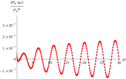
The dependence of the corrected power spectrum is displayed in Fig. 4. Note that, because of Eq. (32), the relative correction to the spectrum of inflaton fluctuations coincides with the correction to the spectrum of ,
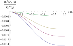
| (74) |
where, using the slow-roll approximation , the spectrum is the one for quasi de Sitter space (qdS). This should be taken into account when physically interpreting the plots in the subsequent Figs. 4–10 because it is the fluctuations in that are directly related to the observable temperature fluctuations (this will be further explained in the discussion section, cf. also (4.1)). The correction to the spectrum vanishes at the initial hypersurface and approaches a non-zero value at . This means that by the end of inflation an imprint of a small black hole on the spectrum will remain.
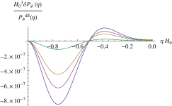
For a homogeneous background the propagator in (double) momentum space contains a delta-peak in the momentum that is associated with the average of the positions. This is seen explicitly in the de Sitter case from Eq. (72). In the case of a small inhomogeneity we find a power law divergence at . The behavior of the spectrum close to this singularity is shown in Fig. 5.

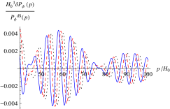
This observation suggests that an expansion in powers of and , which is the basis of the analysis in Ref. [13] is inappropriate for the complete analysis of small black holes in inflation, and, in what follows, we shall not make use of this expansion. Instead, we shall analyze the mixed space spectrum without making an expansion in powers of .
From Eqs. (71) and (69) it follows that at the initial hypersurface (). In other words, we consider a primordial black hole that was created at a time , and we study how it perturbs scalar quantum fluctuations during the subsequent inflationary period.
For also holds and we can expand in (69) to get
| (75) | |||
where we kept and unexpanded. From this expression we see that there is a contribution that remains finite at future infinity, i.e. at the end of inflation, meaning that this correction to the spectrum is propagated through the radiation and matter dominated epochs of the Universe. Taking the limit one finds
| (76) | ||||
Note that . Therefore, this contribution to the propagator is subdominant at late times and becomes completely negligible by the end of inflation. Since we are primarily interested in late time cosmology, from now on we shall not consider these terms. However, we should keep in mind that these terms become increasingly important at early times when approaches , since they guarantee that when .
6.2 Mixed space representation
Rather than working with the momentum , we shall mainly consider the mixed space propagator by means of a Fourier transformation of (71) with respect to . The mixed space propagator is a function of the relative momentum , the average position and the times and . This makes the physical interpretation easier, because the corresponding equal time statistical propagator
| (77) |
is closely related to the Boltzmann distribution function (), cf. [40], and hence allows for a simple statistical interpretation as the phase space density of particles with momentum at position at time . Likewise, the corresponding spectrum can be given an analogous simple statistical interpretation. The dependence on as well as on in the mixed space propagator signals a breakdown of translational invariance. Furthermore, the mixed space representation is advantageous also because the power law divergence at , that plagues the double momentum space propagator, will become a mild logarithmic divergence in the mixed space propagator, whose origin is the IR divergence of the BD vacuum. From the above discussion we know that this divergence is regulated when the IR of the de Sitter state is made finite. Just as we have regulated the de Sitter propagator (56), we shall regulate this divergence by placing the Universe in a comoving box of size . The mixed space propagator can then be written as
| (78) | |||
An inspection of this integral shows that it is indeed logarithmically divergent in the IR when , where . The divergence is regulated by imposing . The terms in the integrand that cause this logarithmic divergence go as for small in (the integral is convergent at where ). Let us split into an IR finite part and an IR divergent part. For this we choose the -axis to point in the direction of and keep general, i.e. and , and introduce and . The momenta and are then simply
| (79) |
Furthermore,
| (80) |
The IR limit, , is then given by the point and in the -plane. The other momentum takes the value there. So, we can split the propagator as follows
| (81) | ||||
with
Restricting the momentum to be above some IR cut-off translates to
| (83) |
for . It follows that
| (84) |
We can neglect terms that vanish for . As a result, we obtain an explicit expression for the cut-off dependent part of the propagator
| (85) | |||
The power spectrum is defined by (cf. Eq. (54)),
| (86) |
with . We have already derived the power spectrum for the de Sitter background, equation (55). Hence, we will only be interested in the correction induced by the black hole,
| (87) |
Again, we can make a split into IR finite and IR divergent part,
| (88) |
with
This expression will be added to the numerical results for the finite part to determine the total correction. The finite part is given in terms of an integral in Appendix C, Eq. (118).
7 Numerical results
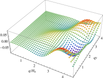
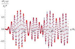
7.1 The anisotropic case: different angles
For we can study the dependence of the spectrum on the angle between and . The numerical results are shown in Fig. 6. All plots show the correction to the spectrum normalized by the scale invariant de Sitter spectrum, Eq. (55),
| (89) |
Although a good fitting curve has not been found for general angles, it is worth noting that besides the high frequency oscillations a modulation with a much lower frequency is present which is determined by the mass parameter . Therefore, the mass of the black hole can, in principle, be inferred directly from the corrections to the scale invariant de Sitter spectrum at large , i.e. at small scales. However, the modes of this magnitude that are stretched into today’s observable scales are due to black holes that were created when the Hubble radius was much smaller than today’s Hubble radius. The probability to find such black holes inside our Hubble volume was estimated in section 3. We will come back to this point in the discussion (see also Fig. 11).

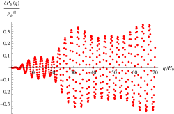
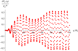
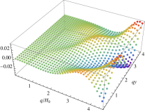
The anisotropic case, , with the vectors and being perpendicular () turns out to be identical within numerical precision to the isotropic case, . From the point of view of observations it is hence impossible to associate data to the one case or the other. On the level of the integral expressions (118, Appendix C) for the two cases one can argue that, because of the pole at , the Bessel function that is present in the anisotropic case is effectively evaluated to unity, yielding the same result as the isotropic case. We demonstrate this in Fig. 7.

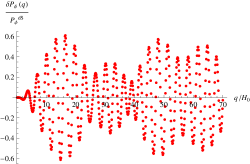
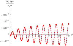
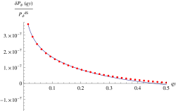
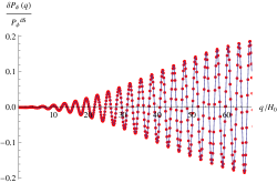
Small values of (large scales) are relevant for black holes that formed at a later stage of inflation although their formation probability is exponentially suppressed (see discussion section). We present numerical results for the spectrum in the region of small and in Fig. 8.
Furthermore, for we can expand and find that
| (90) |
with . This means that the cut-off dependent and cut-off independent part of the correction to the spectrum factorize individually for low momenta. The integral expression of the functions is given in Appendix C, Eq. (120). In Fig. 9 we plot the corrected spectrum for different angles and small . We find that the function is very well approximated by
| (91) |
for any angle . The fit is not very good in the intermediate region . Thus, we have found an analytic expression that describes the correction to the spectrum very well for large scales. Moreover, the mass parameter for the black hole can be found from the amplitude of the spectrum and the IR cut-off from the enveloping curve.
7.2 The isotropic case: cut-off and dependence
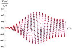
We pointed out in the previous section that the isotropic case virtually coincides with the case that the vectors and are perpendicular but non-zero. Yet, we can study the dependence of the spectrum on and the cut-off . The results are summarized in Fig. 10 with general fitting curves (cf. Appendix D) that approximate the numerical data very well, in particular for small . Again, the mass parameter determines the modulation frequency.
8 Discussion and Conclusion
In this work we have derived the correction to the scale invariant power spectrum of a scalar field on de Sitter space from a small primordial black hole to lowest orders in its mass parameter . To this end, in section 3, we have first analyzed the probability of black hole formation in the pre-inflationary Universe. In order to maximize the formation probability, we have assumed that the pre-inflationary Universe is dominated by heavy non-relativistic particles, in which case sub-Hubble perturbations grow. We have found that there is a range for the particle mass


and the Hubble rate during that period for which the expected number of sub-Hubble black holes per Hubble volume can be larger than , as can be seen in Fig. 3.
To determine the correction to the spectrum in section 5 we have derived an analytic expression for the momentum space propagator of the massless, minimally coupled, scalar field on the Schwarzschild-de Sitter background in the Schwinger-Keldysh formalism. We observe that the propagator diverges in the infrared, demonstrating that, in contrast to a recent proposal [13], an expansion in the momenta is inappropriate, although the breaking of homogeneity is weak. This divergence can be traced to the well known infrared divergence of the massless scalar propagator on de Sitter. We have used a simple regularization, which consists of placing the Universe in a large, but finite, comoving box.


In section 4 we have outlined the procedure which has allowed to determine the impact of an inflationary black holes on the CMB and structure formation. We have demonstrated that, to leading order in the dimensionless black hole mass parameter , the Sasaki-Mukhanov field (curvature perturbation) remains the correct gauge invariant, dynamical scalar perturbation. By working in the zero curvature gauge, we have then shown how to connect the spectrum in the scalar field fluctuation to the spectrum of the comoving curvature perturbation. Finally, the knowledge of the appropriate transfer functions has allowed to relate the inflationary curvature perturbation to the CMB temperature fluctuations and to the large scale structure of the Universe. That analysis is yet to be done in detail. Temperature fluctuations are obtained from fluctuations in the Sasaki-Mukhanov variable by the Sachs-Wolfe effect which yields on large scales
| (92) |
The power spectrum of scalar cosmological perturbations was studied in the mixed representation in the sections 6.2 and 7 and can thus be related to the temperature fluctuations on large scales by performing a Fourier transformation of (92) with respect to . On small scales the more complicated relation (4.1) has to be used, whereby the appropriate transfer functions have to be determined numerically. Other transfer functions have to be used if one wants to study the effect on large scale structure from perturbations of .
The scalar field propagator in the mixed representation is closely related to the Wigner function, and hence admits a probabilistic interpretation characterizing the Boltzmann distribution function. In section 7 we devoted quite some effort to analyze the mixed space spectrum which is a function of not only the relative (comoving) momentum , but also of the comoving black hole distance from us, , of the angle , and finally of the lowest infrared (cut-off) momentum that can be excited. Our results are mostly analyzed as the black hole contribution to the spectrum relative to the scalar contribution in de Sitter space. Since the observed spectrum is highly isotropic, and seemingly homogeneous, we were primarily interested in the case when the perturbation induced by a black hole is small, which led us to consider the limit , or, more precisely, , cf. Eq. (12). The lower limit comes from the requirement that, before it evaporates, the black hole must last at least several e-folds during inflation. The effect of the black hole evaporation during inflation is illustrated in Fig. 2.
The spectrum is first analyzed in section 7.1 for the general anisotropic case, , with the displacement vector of the black hole with respect to us for different angles between and the momentum vector that is conjugate to the relative distance of two points. Then we considered the large scale region ( and small) for the special case that and are parallel. Furthermore, by making an expansion for of the integral expression for the spectrum we showed that it takes a relatively simple form, Eq. (90). We presented an explicit expression for fitting functions for the dependent part which was determined numerically. In the isotropic case, , the dependence on the parameter is shown. Unlike the spectrum of scalar homogeneous perturbations in inflation, which is a function of the momentum magnitude , and depends on two parameters, and at the Hubble crossing, the scalar spectrum in Schwarzschild-de Sitter space depends on , the distance to the black hole and the angle between and . It can serve as a six dimensional template, whereby the template parameters are the comoving black hole position , its mass parameter , and and at the first Hubble crossing during inflation. As a summary of the numerical results we can conclude that (i) the spectrum as a function of is modulated with a lower frequency which is characterized by the mass parameter of the black hole; (ii) the enveloping amplitude of the spectrum scales logarithmically with the IR cut-off , and (iii) the isotropic case cannot be distinguished from a particular configuration of the anisotropic case (where .
We should point out, however, that a comprehensive analysis of the power spectrum of scalar cosmological perturbations induced by small inflationary black holes should take into account also the degrees of freedom of the graviton and start with the action for the scalar field and the graviton on the unperturbed background. In particular, it is important to study the possible mixing of the scalar, vector and tensor modes induced by the black hole. Provided Eq. (32) is an accurate expression for the curvature perturbation in terms of the scalar field perturbation in the inhomogeneous case when a small black hole is present, then based on Eq. (32) one can calculate the spectrum of comoving curvature perturbation induced by an inflationary black hole. This is the quantity of interest since it sources the CMB temperature fluctuations and the large scale structure. Of course, a more realistic inflationary background is a Schwarzschild black hole in a quasi-de Sitter space (SqdS), in which the Hubble rate and the deceleration parameter are both slowly varying functions of time. In order to make sure that the results presented here hold also for that case, one would have to make a complete analysis of cosmological perturbations on a SqdS space, which is beyond the scope of the present work.
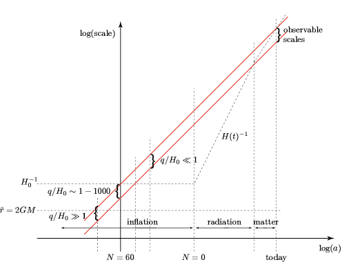
Corrections to the power spectrum from primordial black holes are potentially relevant for observations. To assess this possibility more carefully, we have to establish a relationship between the probability of pre-inflationary black hole formation from section 3 and the expected number of black holes that leave an imprint on today’s CMB sky. A first step in doing that is to trace physical wavelengths, , back in time and check which modes correspond to today’s observable scales. In Fig. 11 it is shown how physical scales are stretched during the evolution of the Universe. The time axis is given in terms of the scale factor . We are interested in the modes which cross for the first time during inflation the Hubble scale at when , evolve on super-Hubble scales until some time in matter (or radiation) era, when they cross the Hubble scale for the second time at . At the end of inflation the ratio of the physical wave length to the Hubble scale will be, , where we assumed that and and constant. Since during radiation and matter era, and , the following relation holds,
| (93) |
where is the scale factor at radiation-matter equality. Neglecting and taking account of the definition, , Eq. (93) yields
| (94) |
Now, recalling that , and , , , Eq. (94) can be recast as
| (95) |
where is the redshift at the second Hubble crossing and is the scale factor today, such that the last term in (95) drops out for modes of the Hubble length today 121212The absence of the graviton signal in the CMB limits (), and hence is an upper limit for the modes with . In Fig. 11 e-folds corresponds to about ()..
The black holes that we have so far considered formed during a pre-inflationary era (). From Fig. 11 we see that if a black hole forms between and and is within our past light-cone then the scales will correspond to observable scales today. Moreover, their amplitude on the CMB will be of the order of of the signal obtained for a homogeneous background, as can be seen
from our numerical results in Figs. 6–10. Such a strong signal has not been observed, implying that such black holes had not formed. If inflation lasted much longer than 60 e-foldings, it would be useful to estimate the probability for black hole formation during inflation. In order to estimate the formation probability in the early stages of inflation, we first note that on sub-Hubble scales Eq. (14) for density perturbations can be used in inflation 131313cf. also Lyth and Liddle ‘The primordial density perturbation’, Cambridge University Press (2009) with the equation of state parameter for matter and the Hubble rate . In slow-roll inflation we can take the Hubble rate to be constant to estimate the growth of the perturbations. Since , the last term in (14) becomes rapidly negligible and we find that the evolution of the perturbation is given by
| (96) |
which means that the leading perturbation tends to a constant. Using the relation between the density perturbation and the fluctuation in the number of particles in the comoving ball with physical radius , Eq. (18), it follows that during inflation ()
| (97) |
where denotes the beginning of inflation. Therefore, also the variance in the fluctuations of is constant for ,
| (98) |
because the average number of particles in a comoving ball does not change during inflation 141414To see this consider the geodesic equation for particles during the inflationary phase, , which shows that their motion (with respect to the fluid rest frame) is exponentially damped, . This means that very quickly particles get frozen and cannot leave the comoving volume, leading to a constant particle number per comoving volume.. Since the universe is dominated by the potential energy of the inflaton field, Eq. (21) is not valid during inflation. Taking this into account, the Friedmann equation is
| (99) |
and we find that the critical fluctuation that is necessary for black hole formation is given by . Considering fluctuations in a volume of radius , we thus obtain the result
| (100) |
In the case when is the comoving radius, , the expression in (100) grows exponentially in physical time. On the other hand, when is a constant physical radius, yields . We conclude from Eq. (25) that the probability for black hole formation is rapidly (faster than exponentially) suppressed during inflation. That means that if inflation lasts much longer than about 70 e-foldings the probability of observing any inflationary black holes within our past light-cone will be tiny. Furthermore, from Figs. 9 and 11 we see that the black holes which form later during inflation (corresponding to ) are observed as and induce unobservably small fluctuations in the CMB. According to the above analysis the probability for formation of these black holes is tiny.
We shall now comment on various ways how this work can be extended. The case of a black hole in inflation can be easily generalized to heavy particles and in particular monopoles by gluing the exterior Schwarzschild-de Sitter geometry to an interior matter solution. The possibility of magnetically charged black holes in the presence of magnetic monopoles is discussed in [41]. Also, it would be interesting to study a rotating body giving rise to an exterior Kerr-de Sitter geometry. Furthermore, there is no reason why a black hole should form in the rest frame of the inflaton field. Assuming a black hole forms with an initial relative speed , its motion will be damped the same way as the motion of a test particle, which obeys a geodesic equation, , such that the speed is Hubble damped as after the formation. Nevertheless, in the early stages after formation the speed of the black hole can yield significant velocity perturbations which may have observational impact on the structure formation, and an interesting question is whether a relation can be established with the recent observation of large scale flows [12]. It is also worth investigating what is the damping of the speed of a spinning massive object.
When this work was nearing completion, we became aware of Refs. [42, 43, 44] which, just like this work, address the problem of scalar field fluctuations on a Schwarz-schild-de Sitter (SdS) background. We note however that there are important differences between these papers and ours, and that our analysis of the black hole perturbations on SdS background is much more elaborate 151515The most important difference is that, in contrast to this work, Cho, Ng and Wang [42] do not make any attempt to relate the inflaton fluctuation to the comoving curvature perturbation, which can be defined on the Schwarzschild-quasi de Sitter space, and which is the correct generalization of homogeneous inflationary spaces. Furthermore, we provide an analytic estimate for the formation probability of small pre-inflationary and inflationary black holes. Next, we provide an exact answer for the Schwinger-Keldysh propagators in the double momentum space (whereby admittedly treating the black hole as a small perturbation on de Sitter space), and we provide a more complete analysis of the significance of the results by discussing how the curvature spectrum gets perturbed as a function of the position of the black hole.. Since the first version of the present paper, several articles have appeared which discuss anomalies in the CMB from black holes and point-like defects. In a recent proposal by Gurzadyan and Penrose [45, 46] the attempt was made to relate the presence of (anomalous) concentric circles in the CMB sky to pre-Big Bang activities involving black holes in the framework of conformal cyclic cosmology. This has been the subject of recent debates [47, 48]. The role of the presence of pre-inflationary particles for anomalies in the CMB was investigated in [22] and [23] where the imprint is also expected to be given in form of rings. Finally, the effect of pre-inflationary black holes on the CMB power spectrum was studied in [49] and a link to the quadrupole anomaly was made.
Acknowledgements. We thank Igor Khavkine, Renate Loll and Albert Roura for helpful discussions.
Appendix A
The coordinate transformations that give rise to the line element in cosmological form, Eq. (2), are presented here.
In its static form the Schwarzschild de Sitter (SdS) solution is given by the line element
| (101) | |||||
with being the Hubble radius and the cosmological constant. This line element reflects the spherical symmetry and the time translation symmetry.
If we take
| (102) |
for then the metric becomes
| (103) |
with
| (104) |
The spatial slices are flat. In order to make the metric diagonal, we have to solve a differential equation for a function
| (105) |
which has the solution
| (106) |
where is a -independent integration constant. This constant can be determined by the requirement that for , i.e. homogeneous cosmology is recovered. One finds that
| (107) |
and hence,
The metric then becomes
| (108) | ||||
which is recast in the main text, Eq. (2), in conformal time , . Note that the metric is singular at
| (109) |
and regular for all values . As a check, , and the Kretschmann invariant is
| (110) |
with denoting as previously the Schwarzschild radial coordinate. This proves that corresponds to the curvature singularity at . Since for , we conclude that when without any double-valued regions.
Appendix B
For the derivation of (5.2) from (62) we have to evaluate first
| (111) | ||||
with the cosine integral function , and . Then, it follows that
| (112) | ||||
To establish (66) and (67) we used the following relations for the step function:
| (113) | |||
The final form for and , Eqs. (69) and (70), can be obtained by solving the following integral, for real parameters and and with ,
| (114) | |||
Appendix C
We present here the general integral expression for the finite part of the spectrum. For this we write
| (115) | ||||
Introducing and , as in the main text, we find that
| (116) |
In terms of the variables and ,
| (117) |
the integral form of the spectrum, in Eqs. (81) and (87–88), becomes
| (118) | ||||
For one finds
| (119) |
with
| (120) | ||||
Appendix D
This appendix contains the fitting functions for the numerical data. In the isotropic case , the correction to the spectrum normalized by the scale invariant de Sitter spectrum has been fitted in Fig. 10 with the following function:
| (121) | |||
We have no analytic expression for the functions and but we observe that the dependence on is weak,
| (122) | |||
Obviously, setting and for all results in reasonable fits, too.
References
- [1] J. C. Mather et al., “Measurement of the Cosmic Microwave Background spectrum by the COBE FIRAS instrument,” Astrophys. J. 420 (1994) 439.
- [2] J. C. Mather, D. J. Fixsen, R. A. Shafer, C. Mosier and D. T. Wilkinson, “Calibrator Design for the COBE Far Infrared Absolute Spectrophotometer (FIRAS),” Astrophys. J. 512 (1999) 511 [arXiv:astro-ph/9810373].
- [3] G. F. Smoot et al., “Structure in the COBE differential microwave radiometer first year maps,” Astrophys. J. 396 (1992) L1.
- [4] W. J. Percival et al., “Baryon Acoustic Oscillations in the Sloan Digital Sky Survey Data Release 7 Galaxy Sample,” Mon. Not. Roy. Astron. Soc. 401 (2010) 2148 [arXiv:0907.1660 [astro-ph.CO]]. B. A. Reid et al., “Cosmological Constraints from the Clustering of the Sloan Digital Sky Survey DR7 Luminous Red Galaxies,” Mon. Not. Roy. Astron. Soc. 404 (2010) 60 [arXiv:0907.1659 [astro-ph.CO]].
- [5] C. L. Bennett et al., “Seven-Year Wilkinson Microwave Anisotropy Probe (WMAP) Observations: Are There Cosmic Microwave Background Anomalies?,” arXiv:1001.4758 [astro-ph.CO].
- [6] C. J. Copi, D. Huterer, D. J. Schwarz and G. D. Starkman, “Large angle anomalies in the CMB,” arXiv:1004.5602 [Unknown].
- [7] A. de Oliveira-Costa, M. Tegmark, M. Zaldarriaga and A. Hamilton, “The significance of the largest scale CMB fluctuations in WMAP,” Phys. Rev. D 69 (2004) 063516 [arXiv:astro-ph/0307282].
- [8] P. K. Samal, R. Saha, P. Jain and J. P. Ralston, “Testing Isotropy of Cosmic Microwave Background Radiation,” Mon. Not. Roy. Astron. Soc. 385 (2008) 1718 [arXiv:0708.2816 [astro-ph]].
- [9] J. P. Uzan, “Dark energy, gravitation and the Copernican principle,” arXiv:0912.5452 [gr-qc]. T. Buchert, “Dark Energy from Structure - A Status Report,” Gen. Rel. Grav. 40, 467 (2008) [arXiv:0707.2153 [gr-qc]]. S. Rasanen, “Evaluating backreaction with the peak model of structure formation,” JCAP 0804 (2008) 026 [arXiv:0801.2692 [astro-ph]].
- [10] S. Alexander, T. Biswas, A. Notari and D. Vaid, “Local Void vs Dark Energy: Confrontation with WMAP and Type Ia Supernovae,” JCAP 0909 (2009) 025 [arXiv:0712.0370 [astro-ph]].
- [11] B. M. Leith, S. C. C. Ng and D. L. Wiltshire, “Gravitational energy as dark energy: Concordance of cosmological tests,” Astrophys. J. 672 (2008) L91 [arXiv:0709.2535 [astro-ph]]. W. Valkenburg, “Swiss Cheese and a Cheesy CMB,” JCAP 0906 (2009) 010 [arXiv:0902.4698 [astro-ph.CO]].
- [12] A. Kashlinsky, F. Atrio-Barandela, H. Ebeling, A. Edge and D. Kocevski, “A new measurement of the bulk flow of X-ray luminous clusters of galaxies,” Astrophys. J. 712 (2010) L81 [arXiv:0910.4958 [Unknown]].
- [13] S. M. Carroll, C. Y. Tseng and M. B. Wise, “Translational Invariance and the Anisotropy of the Cosmic Microwave Background,” Phys. Rev. D 81, 083501 (2010) [arXiv:0811.1086 [astro-ph]].
- [14] E. Komatsu et al., “Seven-Year Wilkinson Microwave Anisotropy Probe (WMAP) Observations: Cosmological Interpretation,” arXiv:1001.4538 [Unknown].
- [15] P. Candelas, “Vacuum Polarization In Schwarzschild Space-Time,” Phys. Rev. D 21 (1980) 2185. P. Candelas and B. P. Jensen, “The Feynman Green Function Inside A Schwarzschild Black Hole,” Phys. Rev. D 33 (1986) 1596. B. P. Jensen and P. Candelas, “The Schwarzschild Radial Functions,” Phys. Rev. D 33 (1986) 1590 [Erratum-ibid. D 35 (1987) 4041].
- [16] E. Winstanley and P. M. Young, “Vacuum polarization for lukewarm black holes,” Phys. Rev. D 77 (2008) 024008 [arXiv:0708.3820 [gr-qc]].
- [17] G. C. McVittie, “The mass-particle in an expanding universe,” Mon. Not. Roy. Astron. Soc. 93 (1933) 325
- [18] G. W. Gibbons and S. W. Hawking, “Cosmological Event Horizons, Thermodynamics, And Particle Creation,” Phys. Rev. D 15 (1977) 2738.
- [19] B. J. Carr and S. W. Hawking, “Black holes in the early Universe,” Mon. Not. Roy. Astron. Soc. 168 (1974) 399.
- [20] H. Saida, T. Harada and H. Maeda, “Black Hole Evaporation in an Expanding Universe,” Class. Quant. Grav. 24 (2007) 4711 [arXiv:0705.4012 [gr-qc]].
- [21] H. Georgi and S. L. Glashow, “Unity Of All Elementary Particle Forces,” Phys. Rev. Lett. 32 (1974) 438.
- [22] A. Fialkov, N. Itzhaki and E. D. Kovetz, “Cosmological Imprints of Pre-Inflationary Particles,” JCAP 1002 (2010) 004 [arXiv:0911.2100 [astro-ph.CO]].
- [23] E. D. Kovetz, A. Ben-David and N. Itzhaki, “Giant Rings in the CMB Sky,” Astrophys. J. 724 (2010) 374 [arXiv:1005.3923 [astro-ph.CO]].
- [24] B. J. Carr, “The Primordial Black Hole Mass Spectrum,” Astrophys. J. 201 (1975) 1.
- [25] T. Prokopec and G. Rigopoulos, “Path Integral for Inflationary Perturbations,” arXiv:1004.0882 [gr-qc].
- [26] V. F. Mukhanov, H. A. Feldman and R. H. Brandenberger, “Theory of cosmological perturbations. “Theory of cosmological perturbations. Part 1. Classical perturbations. Part 2. Quantum theory of perturbations. Part 3. Extensions,” Phys. Rept. 215 (1992) 203.
- [27] H. Kodama and M. Sasaki, “Cosmological Perturbation Theory,” Prog. Theor. Phys. Suppl. 78 (1984) 1.
- [28] H. V. Peiris et al. [WMAP Collaboration], “First year Wilkinson Microwave Anisotropy Probe (WMAP) observations: Implications for inflation,” Astrophys. J. Suppl. 148, 213 (2003) [arXiv:astro-ph/0302225].
- [29] J. S. Schwinger, “Brownian motion of a quantum oscillator,” J. Math. Phys. 2, 407 (1961).
- [30] L. V. Keldysh, “Diagram technique for nonequilibrium processes,” Zh. Eksp. Teor. Fiz. 47, 1515 (1964) [Sov. Phys. JETP 20, 1018 (1965)].
- [31] R. D. Jordan, “Effective Field Equations for Expectation Values,” Phys. Rev. D 33 (1986) 444.
- [32] S. Weinberg, “Quantum contributions to cosmological correlations,” Phys. Rev. D 72 (2005) 043514 [arXiv:hep-th/0506236].
- [33] N. D. Birrell and P. C. W. Davies, “Quantum Fields In Curved Space,” Cambridge, UK: University Press (1982).
- [34] A. Vilenkin and L. H. Ford, “Gravitational Effects Upon Cosmological Phase Transitions,” Phys. Rev. D 26 (1982) 1231.
- [35] T. M. Janssen and T. Prokopec, “Regulating the infrared by mode matching: A massless scalar in expanding spaces with constant deceleration,” arXiv:0906.0666 [gr-qc].
- [36] T. S. Koivisto and T. Prokopec, “Quantum backreaction in evolving FLRW spacetimes,” arXiv:1009.5510 [gr-qc].
- [37] N. C. Tsamis and R. P. Woodard, “Strong infrared effects in quantum gravity,” Annals Phys. 238 (1995) 1.
- [38] N. C. Tsamis and R. P. Woodard, “The Physical basis for infrared divergences in inflationary quantum gravity,” Class. Quant. Grav. 11 (1994) 2969.
- [39] T. Prokopec and E. Puchwein, “Photon mass generation during inflation: de Sitter invariant case,” JCAP 0404 (2004) 007 [arXiv:astro-ph/0312274].
- [40] B. Garbrecht, T. Prokopec and M. G. Schmidt, “Particle number in kinetic theory,” Eur. Phys. J. C 38 (2004) 135 [arXiv:hep-th/0211219].
- [41] W. A. Hiscock, “Magnetic Monopoles And Evaporating Black Holes,” Phys. Rev. Lett. 50 (1983) 1734.
- [42] H. T. Cho, K. W. Ng and I. C. Wang, “Scalar field fluctuations in Schwarzschild-de Sitter space-time,” arXiv:0905.2041 [astro-ph.CO].
- [43] J. E. M. Aguilar and M. Bellini, “Primordial SdS universe from a 5D vacuum: scalar field fluctuations on Schwarzschild and Hubble horizons,” arXiv:1003.1105 [Unknown].
- [44] L. M. Reyes, J. E. M. Aguilar and M. Bellini, “Stochastic emergence of inflaton fluctuations in a SdS primordial universe with large-scale repulsive gravity from a 5D vacuum,” arXiv:1005.1232 [Unknown].
- [45] V. G. Gurzadyan and R. S. Penrose, “Concentric circles in WMAP data may provide evidence of violent pre-Big-Bang activity,” arXiv:1011.3706 [astro-ph.CO].
- [46] V. G. Gurzadyan and R. S. Penrose, arXiv:1012.1486 [astro-ph.CO].
- [47] I. K. Wehus and H. K. Eriksen, “A search for concentric circles in the 7-year WMAP temperature sky maps,” arXiv:1012.1268 [astro-ph.CO].
- [48] A. Hajian, “Are There Echoes From The Pre-Big Bang Universe? A Search for Low Variance Circles in the CMB Sky,” arXiv:1012.1656 [astro-ph.CO].
- [49] F. Scardigli, C. Gruber and P. Chen, “Black Hole Remnants in the Early Universe,” arXiv:1009.0882 [gr-qc].