Stationary entanglement in $N$-atom subradiant degenerate cascade systems

Abstract

We address ultracold $N$-atom degenerate cascade systems and show that stationary subradiant states, already observed in the semiclassical regime, also exist in a fully quantum regime and for a small number of atoms. We explicitly evaluate the amount of stationary entanglement for the two-atom configuration and show full inseparability for the three-atom case. We also show that a continuous variable description of the systems is not suitable to detect entanglement due to the nonGaussianity of subradiant states.

I Introduction

Atomic subradiant states have recently gained wide attention because of their exceptionally slow decoherence Dicke ; Haroche . This stability of quantum superpositions inside the subradiant subspaces originates from the low probability of photon emission, which means very weak interaction between the atoms and their environment. Hence, the subradiant states span a decoherence-free subspace Zurek ; Foldi ; Lidar of the atomic Hilbert space, and consequently, can become important from the viewpoint of quantum computation Plenio ; Beige .

Subradiance in an extended pencil-shaped sample has been observed in an unique experiment in 1985 by Pavolini et al. Pavolini . Among different schemes of multilevel systems, Crubellier et al.Cru1 ; Cru2 ; Cru3 ; Cru4 investigated in detail the arising of subradiance in three-level atoms with a degenerate transition. More precisely, they considered the case of three-level atoms with two transitions sharing either the upper level (’$\Lambda$ configuration) or the lower level (’$V$’ configuration) or the intermediate one (’cascade’ configuration), when both the transitions have the same frequency and the same polarization. The first two configurations may be experimentally realized by rather specific atomic level systems, having a small hyperfine structure, whereas the degenerate cascade configuration, which contains two cascading transitions of the same frequency, would in fact be encountered in atomic-level systems only in the presence of an external field which suitably modifies the atomic frequencies Cru2 . Recently, the same degenerate cascade among three equally spaced levels has been investigated for collective momentum states of an ultracold atomic gas in a high-finesse ring cavity driven by a two-frequency laser field Piovella . This system is particularly attractive for the observation of subradiance, since the absence of Doppler broadening and collisions at sub-recoil temperatures avoid other undesirable decoherence mechanisms. Furthermore, the experimental control of the external parameters, as for instance the intensities of the pump fields, allows for a continuous tuning through different subradiant states of the system, which instead should result difficult or impossible for internal atomic transitions.

More specifically, the system described in Piovella consists in $N$ two-level ultracold bosonic atoms (at $T\approx 0$) placed in a ring cavity with linewidth $\kappa$ and driven by two pump fields $E_{0}$ and $E_{1}$ of frequency $\omega$ and $\omega+\Delta$, respectively. The atoms scatter the photons of the two-frequency pump into a single counterpropagating cavity mode. The pump frequency $\omega$ is sufficiently detuned from the atomic resonance $\omega_{0}$ to neglect absorption. The scattering process can be described by two steps. In the first step the atom, initially at rest, scatters the $\omega$ pump photon into a photon with frequency $\omega_{s1}=\omega-\omega_{r}$, and recoils with a momentum $\vec{p}=\hbar\vec{q}$ (where $\vec{q}=\vec{k}-\vec{k}_{s}$ is the transferred momentum, $\omega_{r}=\bar{q}^{2}/2M$ is the recoil frequency and $M$ is the atomic mass). In the second step the atom scatters the $\omega+\Delta$ pump photon into a photon with frequency $\omega_{s2}=\omega+\Delta-3\omega_{r}$, changing momentum from $\vec{p}=\hbar\vec{q}$ into ${\vec{p}}\,^{\prime}=2\hbar\vec{q}$. The recoil shift of $3\omega_{r}$ arises from the kinetic energy conservation, i.e. $\Delta E=(p^{\prime 2}-p^{2})/2M=3\hbar\omega_{r}$. If the frequency difference between the two pump fields is $\Delta=2\omega_{r}$, then $\omega_{s1}=\omega_{s2}\equiv\omega_{s}$ and a degenerate cascade between three momentum levels, $\vec{p}=m(\hbar\vec{q})$, with $m=0,1,2$, is realized. Furthermore, if the cavity linewidth $\kappa$ is smaller that $2\omega_{r}$, the cavity will support only a single frequency $\omega_{s}$, avoiding further higher-order scattering with frequency $\omega_{s}\pm m\omega_{r}$. In this way the transitions are restricted to only the first three momentum states, forming a three-level degenerate cascade. Although the condition $\kappa\ll 2\omega_{r}$ is experimentally demanding, requiring a typical cavity finesse larger than $10^{6}$, it is not very far from the state-of-art optical cavities Tub ; Hammerich . An important feature of the momentum three-level cascade is that the ratio of the two transition rates is $\epsilon=|E_{1}/E_{0}|$, i.e. it is an experimentally tunable parameter, contrarily to the case of atomic transitions where it is fixed by the branching ratios.

In this paper we address $N$-atom degenerate cascade systems and show that stationary subradiant states also exist in a fully quantum regime. Actually, the action of the coupling to the environment drives our system into an entangled state without the need of isolating it from the rest of the universe. We solve explicitly the Master equation governing the system for a small number of atoms and evaluate the amount of stationary entanglement ETC . In turn, our system represents an example of robust generation of steady state entanglement among atoms via the interaction with the electromagnetic field which act as an engineered environment 2209 . The paper is structured as follows. In the next Section we give a full quantum description of the dynamics and we numerically solve a quantum master equation for $N=2(3)$-atom systems. In the Section III we study the entanglement properties of subradiant states looking at the system from both discrete-variable and continuous-variable (CV) point of view and show that CV criteria are not able to detect entanglement due to nonGaussianity of subradiant states. Section IV closes the paper with some concluding remarks.

II Dissipative dynamics and N-atom pure subradiant states

The three-level degenerate cascade interaction is described by the following Hamiltonian operator in interaction picture

$$H_{int}=-i\hbar g\left[ac_{1}c_{0}^{\dagger}+\epsilon ac_{2}c_{1}^{\dagger}-\textrm{h.c.}\right]$$ (1)

for the three atomic bosonic operators, $c_{m}$, with $m=0,1,2$ and $[c_{m},c^{\dagger}_{n}]=\delta_{m,n}$, and for the single cavity radiation mode, $a$, with $[a,a^{\dagger}]=1$; $g$ is the coupling constant and $\epsilon$ is the relative rate of the second transition, from $m=1$ to $m=2$. The state of the total system is described by a density operator $\varrho$ which is defined on the overall Hilbert space $\mathcal{H}=\mathcal{H}_{0}\otimes\mathcal{H}_{1}\otimes\mathcal{H}_{2}\otimes\mathcal{H}_{f}$, $\mathcal{H}_{i}$ being the Hilbert-Fock space associated to the $m=i$ atomic mode and $\mathcal{H}_{f}$ the Hilbert-Fock space associated to the radiation mode $a$.
Introducing the Fock states $|n_{0},n_{1},n_{2}\rangle$, where $n_{i}$ is the number of quanta in the $m=i$ mode, it has been demonstrated in Cru2 ; Piovella that such a $N$-atom system, with $N$ even, admits $N/2$ subradiant pure states,

$$|sr\rangle_{p}= C_{p}\sum_{k=0}^{p}\bigg{(}\frac{-1}{2\epsilon}\bigg{)}^{k}\frac{1}{k!}\sqrt{\frac{(2k)!(N-p-k)!}{(p-k)!}}\times$$ (2)

$$|p-k,2k,N-p-k\rangle$$

where

$$C_{p}=\left[\frac{(N-p)!}{p!}\;{{}_{2}}F_{1}(-p\,,1/2\,;-N+p\,;\epsilon^{-2})\right]^{-1/2}$$

where ${{}_{2}}F_{1}(a,b;c;z)$ is the hypergeometric function and $p=1,\dots,N/2$, at whom we can add the ground state $|sr\rangle_{0}=|0,0,N\rangle$ for $p=0$. If $N\gg 1$ these states exist iff $0\leq\epsilon\leq 1+\sqrt{2}$.

In order to study the time-evolution of $\varrho$ accounting for scattered photons dissipation too, in a pure quantum mechanical framework, we introduce the following $T=0$ Lindblad master equation

$$\frac{d}{dt}\varrho=\frac{1}{i\hbar}[H_{int},\varrho]+2\kappa\mathcal{L}[a]\varrho$$ (3)

where $\mathcal{L}[a]\varrho=a\varrho a^{\dagger}-a^{\dagger}a\varrho/2-\varrho a^{\dagger}a/2$ is the Lindblad operator describing the cavity damping of the mode $a$. In the next subsections we solve numerically Eq.(3) for two and three atoms in terms of total Fock states $|n_{0},n_{1},n_{2},n\rangle$, where $n$ is the number of scattered photons. We will find that for every $\epsilon$ and for $\kappa\neq 0$ Eq.(3) always admits a stationary solution of the form

$$\varrho_{s}=\Big{[}P_{1}|sr\rangle_{11}\langle sr|+(1-P_{1})|sr\rangle_{00}\langle sr|\Big{]}\otimes|0\rangle\langle 0|$$ (4)

where $|sr\rangle_{0},|sr\rangle_{1}$ are the only two populated states of two-atom and three-atom systems, $P_{1}=\textrm{Tr}\left\{\varrho|sr\rangle_{1}\,{}_{1}\langle sr|\right\}$ and $|0\rangle$ is the vacuum photon state.

II.1 $N=2$ system

From Eq.(2) it is straightforward to check that the two-atom system admits the subradiant state

$$|sr\rangle_{1} = \frac{1}{\sqrt{1+2\varepsilon^{2}}}(|0,2,0\rangle-\sqrt{2}\varepsilon|1,0,1\rangle).$$ (5)

We choose as initial condition for Eq.(3) $\varrho_{i}=|2,0,0,0\rangle\langle 2,0,0,0|$. Fig.1 (top) shows the time evolution of the populations $\langle N_{i}\rangle=\textrm{Tr}[c_{i}^{\dagger}c_{i}\varrho]$ (with $i=0,1,2$) and $\langle N\rangle=\textrm{Tr}[a^{\dagger}a\varrho]$ for chosen values of $\kappa$ and $\epsilon$: we observe that $\langle N_{0}\rangle$ and $\langle N_{1}\rangle$ tend to non-zero values after the photons have escaped from the cavity. This result suggests that the atoms do not decay to the lower momentum state $m=2$, but they arrange themselves in a superposition of the three momentum states. Fig.2 (top) shows the time evolution of the probabilities $P_{i}=\textrm{Tr}[\varrho|sr\rangle_{ii}\langle sr|]$, for $i=0,1$, for the same values of $\kappa$ and $\epsilon$. Asymptotically, $P_{0}+P_{1}=1$ and $\varrho$ approaches the steady-state density matrix $\varrho_{s}$ of Eq.(4), where $P_{1}$ in general is a function of the parameters $\epsilon$ and $\kappa$. A similar behavior may be observed for any choice of the interaction parameters. In the bad-cavity limit, $\kappa\gg g$, Eq. (3) is well approximated by the following effective superradiant master equation Cru2 ; Boni

$$\frac{d\varrho_{a}}{dt}=\Gamma S^{-}\varrho_{a}S^{+}-\frac{\Gamma}{2}(S^{+}S^{-}\varrho_{a}+\varrho_{a}S^{+}S^{-})$$ (6)

where $\varrho_{a}$ is the atomic density operator, $S^{-}=c_{1}^{\dagger}c_{0}+\varepsilon c_{2}^{\dagger}c_{1}$ and $\Gamma=g^{2}/\kappa$. Solving this equation analytically we get an expression for the time-evolution of $P_{1}$ and in the stationary limit we find a $\Gamma$-independent expression

$$P_{1}=\frac{2(1-\epsilon^{2})^{2}}{9\epsilon^{2}+2(1-\epsilon^{2})^{2}}$$ (7)

This expression is in excellent agreement with the solutions of Eq. (3) for any possible value of $\epsilon$ in the bad cavity regime. In Fig.3 (top) we see that $P_{1}$ decreases from unit as $\epsilon$ increases and it vanishes for $\epsilon=1$, for which the degenerate three-level cascade has equal transition rates and the atoms decay superradiantly to the ground state. For $\epsilon>1$ the subradiant probability increases and reaches asymptotically the unity. For large values of $\epsilon$ the steady-state is no longer a mixed state, $\varrho_{s}\approx|1,0,1\rangle\langle 1,0,1|$.

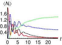
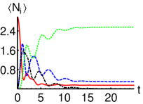
Figure 1: Time evolution of $\langle N_{i}\rangle$ for $m=0$ (red), $m=1$ (blue dashed), $m=2$ (green dotted) and $\langle N_{ph}\rangle$ (black dot-dashed) with $t$ in unit of $1/g$. Left: $N=2$, $\kappa=0.2g,\epsilon=0.3$. Right: $N=3$, $\kappa=0.3g,\epsilon=0.5$.

II.2 $N=3$ system

In this case we cannot directly use the eq.(2) which applies only for $N$ even. The equation $S^{-}|\psi\rangle=0$, where $|\psi\rangle$ is a generic three-atom state, is satisfied by the subradiant state

$$|sr\rangle_{1} = \frac{1}{\sqrt{1+4\epsilon^{2}}}(|0,2,1\rangle-2\epsilon|1,0,2\rangle)$$ (8)

Fig.1 (bottom) shows the time evolution of the populations $\langle N_{i}\rangle$ with $i=0,1,2$ and $\langle N\rangle$ for fixed values of $\epsilon$ and $\kappa$, obtained solving Eq.(3) with initial condition $\varrho_{i}=|3,0,0,0\rangle\langle 3,0,0,0|$. As in the $N=2$ case the mean occupation number of every atomic mode saturates to non-zero values and, asymptotically, the only atomic states surviving are the subradiant state $|sr\rangle_{1}$ and the ground state $|sr\rangle_{0}=|0,0,3\rangle$. Hence also in this case we can write the reduced steady-state density operator in the form (4). Fig.2 (bottom) shows $P_{1}$ vs $t$ and Fig.3 (top) vs $\epsilon$ for a particular choice of $\kappa$. There are some important differences and analogies with the $N=2$ case. First we note that this time $P_{1}$ vanishes for $\epsilon=0$, whereas in the $N=2$ case it has a maximum and is equal to unity. This is a consequence of the fact that the two-atom subradiant state (5) contains the state $|0,2,0\rangle$ which is the ground state for $\epsilon=0$ (only the $m=0\rightarrow m=1$ transition can take place). On the contrary, for $N=3$ the steady-state density operator does not contain the state $|0,3,0\rangle$ which is the three-atom analogue; moreover, it is a linear superposition of states with $n_{2}\neq 0$ so, if the second transition is forbidden, it is impossible to populate these states observing subradiance. Secondly, whereas for $N=2$ $P_{1}$ decreases increasing $\epsilon$ and vanishes for $\epsilon=1$, for $N=3$ $P_{1}$ increases, it reaches a maximum around $\epsilon\approx 0.5$ and decreases again falling off to zero for $\epsilon=1$. For $\epsilon>1$ the behavior of the two plots is quite similar.

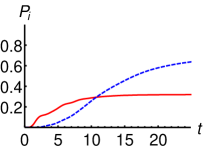
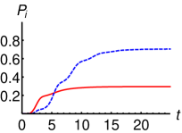
Figure 2: Time evolution of $P_{0}$ (blue dotted) and $P_{1}$ (red) with $t$ in unit of $1/g$. Left: $N=2$, $\kappa=0.2g,\epsilon=0.3$; Right: $N=3$, $\kappa=0.3g,\epsilon=0.5$.

II.3 Large $N$ and p-degeneracy

Let us consider now the $N\gg 1$. In Piovella the following relation linking the $p$-index and $\epsilon$ has been given:

$$p =\frac{N}{2}\left(\frac{1-2\epsilon^{2}}{1-\epsilon^{2}}\right)\qquad 0\leq\epsilon\leq 1/\sqrt{3}$$ (9)

$$p =N\left(\frac{1-\epsilon^{2}}{1+\epsilon^{2}}\right)^{2}\quad 1/\sqrt{3}\leq\epsilon\leq 1+\sqrt{2}$$ (10)

Let us pay more attention to formulas (10). For $1/\sqrt{3}\leq\epsilon\leq\sqrt{3}$ it is easy to prove that they exist two different values of $\epsilon$ corresponding to the same value of $p$ (except for $\epsilon=1$ yielding $p=0$ i.e. the ground state). This means that, once $p$ is fixed, the two subradiant states $|sr\rangle_{p(\epsilon_{0})},|sr\rangle_{p(\epsilon_{1})}$ are both acceptable, provided that they are actually different states. Now, let us assume that, for a fixed $p$, it is possible to build the following two states:

$$|\psi^{(\pm)}_{p}\rangle=\frac{1}{\sqrt{2}}(|sr\rangle_{p(\epsilon_{0})}\pm|sr\rangle_{p(\epsilon_{1})}).$$ (11)

It is straightforward to show that the two following states are orthonormal

$$|\phi^{(\pm)}_{p}\rangle=\frac{1}{\sqrt{1\pm\alpha}}|\psi^{(\pm)}_{p}\rangle$$ (12)

where $\alpha=\,_{p(\epsilon_{0})}\langle sr|sr\rangle_{p(\epsilon_{1})}=\,_{p(\epsilon_{1})}\langle sr|sr\rangle_{p(\epsilon_{0})}\in\mathbb{R}$. We can compute the total kinetic energy of the condensate and also the energy difference between these two states $|\Delta_{p}|=|E_{p}^{(+)}(\epsilon)-E_{p}^{(-)}(\epsilon)|$ which turns out to be

$$|\Delta_{p}|= \bigg{|}\frac{4(2N-2p-2[\bar{k}(\epsilon_{0}(p))+\bar{k}(\epsilon_{1}(p))])}{\sqrt{2(1+\alpha)}}-$$ (13)

$$\frac{2[\bar{k}(\epsilon_{0}(p))+\bar{k}(\epsilon_{1}(p))]}{\sqrt{2(1-\alpha)}}\bigg{|}$$

where

$$\bar{k}(\epsilon_{j}(p))= \frac{p!(N-p-1)!}{2\epsilon_{j}^{2}(N-p)!(p-1)!}\times$$

$$\frac{{{}_{2}}F_{1}(1-p,3/2;1+p-N;\epsilon_{j}^{-2})}{{{}_{2}}F_{1}(-p,1/2;p-N;\epsilon_{j}^{-2})}.$$

Since this parameter depends on $\epsilon$, in principle it should be possible to distinguish between the two states (12). More interesting, by applying an external potential coupling these two states, we could realize a fictitious two-level system where the many-body states $|\phi^{(\pm)}_{p}\rangle$ play the role of the logical-basis states $|0\rangle,|1\rangle$. A similar system has been proposed in Keitel for a $\Lambda$ configuration.

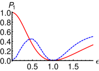
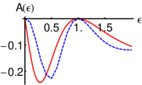
Figure 3: Left: steady state probability as a function of $\epsilon$ for $N=2$ (red) and $N=3$ (blue dashed). Right: negative eigenvalue of the partially transposed state as a function of $\epsilon$ for $N=2$ (red) and $N=3$ (blue dashed). In the $N=3$ case we have set $\kappa=0.8g$.

III Entanglement properties

In this section we address the entanglement properties of the state (4) either regarded as made of three bosonic modes or, upon considering the selection rule induced by the constraint on the number of atoms, as a finite dimensional one. Generally speaking, there are several classes of entanglement in a tripartite quantum system, from genuine tripartite entanglement to full separability passing through bipartite separability, which are defined on the basis of all possible groupings of the three parties tre . Our primary goal is to establish whether the stationary state is fully inseparable and if it is possible to quantify the amount of entanglement.

At first, we notice that our system consists of three atomic modes for which, being the atomic ensemble made of a finite and fixed number of atoms, only a finite number of quanta per mode is permitted from a minimum of $n_{i}=0$ up to a maximum of $n_{i}=N$. This physical constraint corresponds to a geometrical constraint which identifies a subspace $\mathcal{S}$ of $\mathcal{H}_{a}=\mathcal{H}_{0}\otimes\mathcal{H}_{1}\otimes\mathcal{H}_{2}$ defined as

$$\mathcal{S}=\left\{\varrho\in\mathcal{H}\ :\sum_{i=0}^{2}\langle N_{i}\rangle=N\right\}\>.$$

Hence, being $\mathcal{S}$ a finite dimension subspace, we can make use of the PPT (Positive Partial Transposition) criterion for discrete-variable quantum systems. In fact, PPT condition is sufficient to establish entanglement of a state and, as we will see, it is enough to show that $\varrho_{s}$ is genuinely tripartite entangled. Partially transposing with respect to a given party corresponds to a specific grouping of two parties with respect to the third: for example when we partial-transpose with respect to the $m=0$ mode we are grouping together the $m=1$ and $m=2$ modes with respect to $m=0$. Suppose we have partial-transposed with respect to $m=0$, obtaining $\varrho_{s}^{T_{0}}$ and let the eigenvalues of $\varrho_{s}^{T_{0}}$ be $\{\lambda_{k}^{(0)}\}$. If it exists at least one $k$ such that $\lambda_{k}<0$ we can conclude that $\varrho_{s}\neq\sum_{j}p_{j}\,\varrho_{j}^{0}\otimes\varrho_{j}^{12}$. If the positivity condition is violated for $\varrho_{s}^{T_{1}}$ and $\varrho_{s}^{T_{2}}$ too we can state that $\varrho_{s}$ is genuinely tripartite entangled. We start with the $N=2$ case and we take the reduced density operator $\textrm{Tr}_{ph}[\varrho_{s}]$ where $\varrho_{s}$ is given by eq.(4) with $P_{1}$ given by eq.(7). The $\mathcal{S}$ subspace is spanned by six Fock states: $|2,0,0\rangle,|0,2,0\rangle,|0,0,2\rangle,|1,1,0\rangle,|1,0,1\rangle,|0,1,1\rangle$. If we compute the eigenvalues of every $\varrho_{s}^{T_{j}}$ with $j=0,1,2$ we find that it always exists a negative eigenvalue $A_{2}(\epsilon)$

$$A_{2}(\epsilon) =-\frac{\sqrt{2}}{2}\frac{\epsilon(\epsilon^{2}-1)^{2}}{(\frac{1}{2}+\epsilon^{2})^{2}(2+\epsilon^{2})}$$

$$=-\frac{\epsilon^{2}(2\epsilon^{2}+3)^{2}+2}{4\sqrt{2}(\epsilon^{2}-1)^{2}}\langle N_{0}\rangle\langle N_{1}\rangle$$ (14)

where the expression on the second line provides a link between the negative eigenvalue, which directly quantifies the amount of entanglement, and a couple of moments which are, at least in principle, amenable to direct measurements.

In the $N=3$ case $\mathcal{S}$ is spanned by the following ten states: $|3,0,0\rangle$, $|0,3,0\rangle$, $|0,0,3\rangle$, $|2,1,0\rangle$, $|2,0,1\rangle$, $|0,1,2\rangle$, $|0,2,1\rangle$, $|1,0,2\rangle$, $|1,2,0\rangle$, $|1,1,1\rangle$ and the PPT condition is still quite simple to employ to establish tripartite entanglement. On the other hand, for $N=3$ we have not been able to give an analytical expression for $P_{1}$ and therefore we resort numerical evaluation of the eigenvalues. As in the previous case we find a negative eigenvalue $A_{3}(\epsilon)$ which turns out to be always the same for every possible partial transposition and for any value of $\epsilon$. This means that also the three-atom $\varrho_{s}$ is genuinely tripartite entangled. Fig.3 (bottom) shows the behavior of $A_{N}(\epsilon)$ both for $N=2$ and $N=3$. The behavior is qualitatively the same for both cases. The eigenvalues decrease from zero and reach a minimum after which they start to increase. As we should expect they vanish for $\epsilon=1$ and after this they start to decrease again.

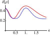
Figure 4: Up: $\delta[\varrho]$ for $N=50$ vs. $\epsilon$ accounting for relations (9)-(10). Bottom: $\delta[\varrho]$ for $N=2$ (red) and $N=3$ (blue dashed); in this second case we have set $\kappa=0.8g$.

III.1 Continuous variable description

Let us now investigate the entanglement properties of our system as a continuous variable one Wal09 , i.e. taking into account that we are dealing with three bosonic modes describing the number of atoms within a given state (for instance momentum state). To this aim we start by reviewing few facts about the description of a multimode continuous variable system GSI . Upon introducing the canonical operators $q_{j}=(c_{j}+c_{j}^{\dagger})/\sqrt{2}$ and $p_{j}=i(c_{j}^{\dagger}-c_{j})/\sqrt{2}$ in terms of the single-mode operators $c_{j}$, $j=0,1,2$ we may write the vector of operators $\boldsymbol{R}=(q_{1},p_{1},q_{2},p_{2},q_{3},p_{3})^{T}$. The so-called vector of mean values $\boldsymbol{X}=\boldsymbol{X}[\varrho]$ and covariance matrix (CM) $\boldsymbol{\sigma}=\boldsymbol{\sigma}[\varrho]$ of a quantum state $\varrho$ have components $X_{j}=\langle R_{j}\rangle$ and $R\sigma_{jk}=\frac{1}{2}\langle\{R_{j},R_{k}\}\rangle-\langle R_{j}\rangle\langle R_{j}\rangle$ where $\langle O\rangle=\textrm{Tr}[\varrho\,O]$ and $\{A,B\}=AB+BA$ denotes the anticommutator. The characteristic function $\chi[\varrho](\boldsymbol{\lambda})=\textrm{Tr}[\varrho\,D(\boldsymbol{\lambda})]$ is defined in terms of the multimode displacement operator $D(\boldsymbol{\lambda})=\otimes_{j=1}^{n}D(\lambda_{j})$, with $\boldsymbol{\lambda}=(\lambda_{1},\cdots,\lambda_{n})^{T}$, $\lambda_{j}\in\mathbb{C}$ and $D(\lambda_{j})=\exp\{\lambda_{j}c_{j}^{\dagger}-\lambda_{j}^{*}c_{j}\}$. A quantum state $\varrho_{G}$ is referred to as a Gaussian state if its characteristic function has the Gaussian form $\chi[\varrho_{G}](\boldsymbol{\Lambda})=\exp\left\{-\frac{1}{2}\boldsymbol{\Lambda}^{T}\boldsymbol{\sigma}\boldsymbol{\Lambda}+\boldsymbol{X}^{T}\boldsymbol{\Omega}\boldsymbol{\Lambda}\right\}$ where $\boldsymbol{\Lambda}$ is the real vector $\boldsymbol{\Lambda}=(\mathfrak{Re}\lambda_{1},\mathfrak{Im}\lambda_{1},\cdots,\mathfrak{Re}\lambda_{n},\mathfrak{Im}\lambda_{n})$ and $\boldsymbol{\Omega}$ is the symplectic matrix $\boldsymbol{\Omega}=i\oplus_{j=1}^{n}\sigma_{2}$, $\sigma_{2}$ being the $y$ Pauli matrix. Gaussian states are thus completely characterized by their mean values vector and their covariance matrix. For bipartite Gaussian states, the PPT condition is necessary and sufficient for separability Sim , and it may be rewritten in terms of the CM, which uniquely determines the entanglement properties of the state under investigation. A mode of a Gaussian state is separable from the others iff $\Lambda_{j}\boldsymbol{\sigma}\Lambda_{j}+\frac{i}{2}\boldsymbol{\Omega}\geq 0$, where $\Lambda_{j}$ is a diagonal matrix implementing the partial transposition at the level of CM, i.e. inverting the sign of the $j$-th momentum. In our case $\Lambda_{1}=\hbox{Diag}(1,-1,1,1,1,1)$, $\Lambda_{2}=\hbox{Diag}(1,1,1,-1,1,1)$, $\Lambda_{3}=\hbox{Diag}(1,1,1,1,1,-1)$. When we have a non Gaussian state the violation of the above condition is still a sufficient condition for entanglement, whereas the necessary part is lost.

Let us start by focusing attention on a $N$-atom pure subradiant state (2). The density operator is $\varrho_{p}=|sr\rangle_{pp}\langle sr|$ and the only non-vanishing terms of the CM $\boldsymbol{\sigma}[\varrho_{p}]$ are the diagonal ones, which are reported in appendix A. This fact is a direct consequence of two selection rules affecting the geometrical form of subradiant states: the first one is the conservation of the number of atoms and the second one is the presence of the $k$-index in every Fock component of $|sr\rangle_{p}$. As a matter of fact, the CM $\boldsymbol{\sigma}[\varrho_{p}]$ satisfies the three separability conditions $\Lambda_{j}\boldsymbol{\sigma}\Lambda_{j}+\frac{i}{2}\boldsymbol{\Omega}\geq 0$, $j=1,2,3$ and therefore we have no information about the entanglement properties of $\varrho_{p}$, i.e. we cannot use the PPT condition translated to continuous-variable systems to analyze and quantify entanglement. On the other hand, we know from the previous analysis that $\varrho_{p}$ is genuinely tripartite entangled state and this suggests that it should be far from being a Gaussian state. Indeed, the characteristic function is given by a Gaussian modulated by Laguerre polynomials and thus shows a distinctive nonGaussian shape.

In the following we will evaluate quantitatively the nonGaussianity of the subradiant states upon the use of the nonGaussianity (nonG) measure introduced in NG1 , which is defined as

$$\delta[\varrho]=\frac{D_{HS}^{2}[\varrho,\tau]}{\mu_{\varrho}}=\frac{\mu_{\varrho}+\mu_{\tau}-2\kappa_{\varrho\tau}}{2\mu_{\varrho}}$$ (15)

where $D_{HS}[\varrho,\tau]$ denote Hilbert-Schmidt distance between the state $\varrho$ under scrutiny and its reference Gaussian state $\tau$, i.e. a Gaussian state with the same mean value $\boldsymbol{X}[\tau]=\boldsymbol{X}[\varrho]$ and CM $\boldsymbol{\sigma}[\tau]=\boldsymbol{\sigma}[\varrho]$, $\mu_{\varrho}=\textrm{Tr}[\varrho^{2}]$ is the purity of $\varrho$, and $\kappa_{\varrho\tau}=\textrm{Tr}[\varrho\,\tau]$ is the overlap between $\varrho$ and $\tau$. The nonG measure $\delta[\varrho]$ possesses all the properties for a good measure of the non-Gaussian character and, in particular, $\delta[\varrho]=0$ iff $\varrho$ is a Gaussian state. For the pure subradiant states $\varrho_{p}=|sr\rangle_{pp}\langle sr|$ the reference Gaussian state has the form $\tau=\nu_{0}\otimes\nu_{1}\otimes\nu_{2}$ where $\nu_{j}=(1-y_{j})\sum_{s}y_{j}^{s}|s\rangle\langle s|$, $y_{j}=N_{j}/(1+N_{j})$ is a (Gaussian) thermal state with $N_{j}$ average thermal photons. For a three-mode thermal state we have $\sigma_{11}=\sigma_{22}=\frac{1}{2}(N_{0}+\frac{1}{2})$, $\sigma_{33}=\sigma_{44}=\frac{1}{2}(N_{1}+\frac{1}{2})$, $\sigma_{55}=\sigma_{66}=\frac{1}{2}(N_{2}+\frac{1}{2})$. Since for a subradiant state the average occupation numbers are given by $N_{0}=p-\langle k\rangle_{p}$, $N_{1}=2\langle k\rangle_{p}$, $N_{2}=N-p-\langle k\rangle_{p}$ we have, after some calculations, that the non-Gaussianity of $\varrho_{p}$ is given by

$$\delta[\varrho_{p}] =\frac{1}{2}+\frac{1}{2}\prod_{j=0}^{2}\frac{1-y_{j}}{1+y_{j}}-|C_{p}|^{2}\prod_{j=0}^{2}(1-y_{j})$$

$$\times\sum_{k=0}^{p}\beta_{k}^{2}\,y_{0}^{p-k}\,y_{1}^{2k}\,y_{2}^{N-p-k}$$ (16)

For a large number of atoms $N\gg 1$ the nonGaussianity of $\delta[\varrho_{p}]$ may be evaluated upon exploiting the Eq. (9)(10) i.e. the relation between $p$ and $\epsilon$. In practice, every value of $\epsilon$ corresponds to a single $p$ and in turn to the pure subradiant state $\varrho_{p}$. In Fig.4 (top) we show the behavior of the nonGaussianity $\delta[\varrho_{p}]$ for $N=50$ and $0\leq\epsilon\leq 1+\sqrt{2}$. As it is apparent from the plot, the subradiant states are always non-Gaussian and the value of $\delta$ is almost constant. For $N=2,3$ it is possible to evaluate explicitly the non-gaussianity for the stationary state (4). Since the number of atoms is small $p$ and $\epsilon$ are independent one another and we are not allowed to use relations (9)-(10). For $N=2,3$ we have the ground state, $\varrho_{0}$, and a single subradiant state, $\varrho_{1}$, and the nonGaussianity may be expressed as

$$\delta[\varrho_{s}]=P_{1}(P_{1}-1)+\frac{1+\mu_{\tau}}{2}-(1-P_{1})\kappa_{\varrho_{0}\tau}-P_{1}\kappa_{\varrho_{1}\tau}\>.$$

The reference Gaussian state is again a three-mode thermal state, as it can be easily demonstrated by noticing that the CM of $\varrho_{s}$ is the convex combination of those corresponding to $\varrho_{0}$ and $\varrho_{1}$ i.e. $\boldsymbol{\sigma}[\varrho_{s}]=P_{1}\boldsymbol{\sigma}[\varrho_{1}]+(1-P_{1})\boldsymbol{\sigma}[\varrho_{0}]=P_{1}$. $P_{1}$ is given by eq.(7) for $N=2$ and it may be evaluated numerically for $N=3$. The overlaps are given in appendix B. The behaviour of the nonGaussianity $\delta[\varrho_{s}]$ as a function of $\epsilon$ for $N=2,3$ is shown in Fig. 4 (bottom). Notice that the behaviour of $\delta[\varrho_{s}]$ does not show a strict correlation to that of the negative eigenvalue $A(\epsilon)$ and thus we cannot use nonGaussianity to assess quantitatively the failure of CV PPT condition in detecting stationary entanglement in our system.

IV Conclusions

In this paper we have considered a systems made of $N$ two-level ultracold bosonic atoms in a ring cavity where subradiance appears in the bad cavity limit. We provided a full quantum description of the dynamics and have shown the appearance of stationary entanglement among atoms. We have evaluated the amount of steady state entanglement for $N=2$ and $N=3$ atoms as quantified by the negativity of the partially transposed density matrix. We have also investigated the entanglement properties of the systems as a continuous variable one and have shown that it is not possible to detect entanglement due to the nonGaussian character of subradiant states. It is important to notice that the life time of experimentally demonstrated entangled states is generally limited, due to their fragility under decoherence and dissipation. Therefore, in order to decrease dissipation and decoherence, strict isolation from the environment is usually considered. On the contrary, in our system, the action of the coupling to the environment drives it into a steady entangled state, which is robust with respect to the interaction parameters. Our results pave the way for entanglement characterization entch of subradiant states and suggest further investigations for large number of atoms.

Appendix A CM of the subradiant state

The covariance matrix of the subradiant state $\varrho_{p}=|sr\rangle_{pp}\langle sr|$ is diagonal. The nonzero matrix elements may be expressed as

$$\sigma_{11} =\sigma_{22}=\frac{|C_{p}|^{2}}{2}\sum_{k=0}^{p}\beta_{k}^{2}\left(p-k+\frac{1}{2}\right)$$ (17)

$$=\frac{1}{2}\left(p-\langle k\rangle_{p}-\frac{1}{2}\right)$$

$$\sigma_{33} =\sigma_{44}=\frac{|C_{p}|^{2}}{4}\sum_{k=0}^{p}\beta_{k}^{2}\left(4k+1\right)$$ (18)

$$=\langle k\rangle_{p}+\frac{1}{4}$$

$$\sigma_{55} =\sigma_{66}=\frac{|C_{p}|^{2}}{2}\sum_{k=0}^{p}\beta_{k}^{2}\left(N-p-k+\frac{1}{2}\right)$$ (19)

$$=\frac{1}{2}\left(N-p-\langle k\rangle_{p}+\frac{1}{2}\right)$$

where we have defined

$$\beta_{k}=\left(-\frac{1}{2\epsilon}\right)^{k}\left(\frac{1}{k!}\right)\sqrt{\frac{(2k)!(N-p-k)!}{(p-k)!}}$$

and $\langle k\rangle_{p}=|C_{p}|^{2}\sum_{k=0}^{p}\beta_{k}^{2}k$ is the mean value of $k$ for the $p$-subradiant state.

Appendix B Overlaps

The overlaps $\kappa_{\varrho_{j}\tau}^{(N)}$ between the states $\varrho_{j}$ and their reference Gaussian states for $N$ atoms, which appears in the expression of the nonGaussianity $\delta[\varrho_{s}]$ are given by

$$\kappa^{(2)}_{\varrho_{0},\tau} =\kappa^{(3)}_{\varrho_{0},\tau}=y_{2}^{2}\,\prod_{j=0}^{2}\frac{1-y_{j}}{1+y_{j}}$$

$$\kappa^{(2)}_{\varrho_{1},\tau} =\frac{y_{1}^{2}+2\epsilon^{2}y_{0}\,y_{2}}{1+2\epsilon^{2}}\prod_{j=0}^{2}\frac{1-y_{j}}{1+y_{j}}$$

$$\kappa^{(3)}_{\varrho_{1},\tau} =\frac{y_{2}\left(y_{1}^{2}+4\epsilon^{2}y_{0}\,y_{2}\right)}{1+4\epsilon^{2}}\prod_{j=0}^{2}\frac{1-y_{j}}{1+y_{j}}\>.$$ (20)

References

- (1) R.M. Dicke, Phys. Rev. 93, 439 (1954).
- (2) M.Gross and S. Haroche, Phys. Rep. 93, 301 (1982).
- (3) W.H. Zurek, Prog. Theor. Phys. 89, 281 (1993).
- (4) P. Fo ldi, A. Czirja k, and M.G. Benedict, Phys. Rev. A 63,033807 (2001).
- (5) D.A. Lidar, I.L. Chuang, and K.B. Whaley, Phys. Rev. Lett. 81, 2594 (1998).
- (6) M. B. Plenio, S. F. Huelga, A. Beige, and P.L. Knight, Phys. Rev. A 59, 2468 (1999).
- (7) A. Beige, D. Braun, B. Tregenna, and P.L. Knight, Phys. Rev. Lett. 85, 1762 (2000).
- (8) D. Pavolini, A. Crubellier, P. Pillet, L. Cabaret, and S. Liberman, Phys. Rev. Lett. 54, 1917 (1985).
- (9) A. Crubellier, S. Liberman, D. Pavolini, and P. Pillet, J. Phys. B: At. Mol. Phys. 18, 3811 (1985).
- (10) A. Crubellier, and D. Pavolini, J. Phys. B 19, 2109 (1986).
- (11) A. Crubellier, J. Phys. B 20, 971 (1987).
- (12) A. Crubellier, and D. Pavolini, J. Phys. B 20, 1451 (1987).
- (13) M.M. Cola, D. Bigerni, N. Piovella, Phys. Rev. A 79 53622 (2009).
- (14) S. Slama, G. Krenz, S. Bux, C. Zimmermann, Ph.W. Courteille, Phys. Rev. A 75, 063620 (2007).
- (15) J. Klinner, M. Lindholdt, B. Nagorny, and A. Hemmerich, Phys. Rev. Lett. 96, 023002 (2006).
- (16) M. M. Cola, N. Piovella, M. G. A. Paris, Phys. Rev. A 70, 043809 (2004).
- (17) C. A. Muschik, E. S. Polzik, J. I. Cirac, preprint arXiv:1007.2209
- (18) R. Bonifacio, P. Schwendimann, and F. Haake, Phys. Rev. A 4, 302 (1971).
- (19) C. Keitel, M. O. Scully, and G. S ussmann, Phys. Rev. A 45, 3242 (1992).
- (20) G. Giedke, B. Kraus, M. Lewenstein, and J. I. Cirac, Phys. Rev. A 64, 052303 (2001).
- (21) R. M. Gomes et al, Proc. Nat. Ac. Sciences 106, 21517 (2009).
- (22) V. D’Auria et al., Phys. Rev. Lett. 102, 020502 (2009).
- (23) A. Ferraro et al., Gaussian States in Quantum Information, (Bibliopolis, Napoli, 2005); G. Adesso et al., J. Phys. A 40, 7821 (2007); S. L. Braunstein et al., Rev. Mod. Phys. 77,513 (2005);
- (24) R. Simon, Phys. Rev. Lett. 84, 2726 (2000).
- (25) M. G. Genoni, M. G. A. Paris, K. Banaszek Phys. Rev. A 76, 042327 (2007).
- (26) M. Genoni, P. Giorda, M. G. A. Paris, Phys. Rev. A 78, 032303 (2008); G. Brida, I. Degiovanni, A. Florio, M. Genovese, P. Giorda, A. Meda, M. G. Paris, A. Shurupov, Phys. Rev. Lett. 104, 100501 (2010).