Adapting to the Shifting Intent of Search Queries

Abstract

Search engines today present results that are often oblivious to abrupt shifts in intent. For example, the query ‘independence day’ usually refers to a US holiday, but the intent of this query abruptly changed during the release of a major film by that name. While no studies exactly quantify the magnitude of intent-shifting traffic, studies suggest that news events, seasonal topics, pop culture, etc account for 50% of all search queries. This paper shows that the signals a search engine receives can be used to both determine that a shift in intent has happened, as well as find a result that is now more relevant. We present a meta-algorithm that marries a classifier with a bandit algorithm to achieve regret that depends logarithmically on the number of query impressions, under certain assumptions. We provide strong evidence that this regret is close to the best achievable. Finally, via a series of experiments, we demonstrate that our algorithm outperforms prior approaches, particularly as the amount of intent-shifting traffic increases.

1 Introduction

Search engines typically use a ranking function to order results. The function scores a document by the extent to which it matches the query, and documents are ordered according to this score. Usually, this function is fixed in the sense that it does not change from one query to another and also does not change over time.

Intuitively, a query is “intent-shifting” if the most desired search result(s) change over time. More concretely, a query’s intent has shifted if the click distribution over search results at some time differs from the click distribution at a later time. For the query ‘tomato’ on the heels of a tomato salmonella outbreak, the probability a user clicks on a news story describing the outbreak increases while the probability a user clicks on the Wikipedia entry for tomatoes rapidly decreases. There are studies that suggest that queries likely to be intent-shifting — such as pop culture, news events, trends, and seasonal topics queries — constitute roughly half of the search queries that a search engine receives [pew].

The goal of this paper is to devise an algorithm that quickly adapts search results to shifts in user intent. Ideally, for every query and every point in time, we would like to display the search result that users are most likely to click. Since traditional ranking features like PageRank [pagerank] change slowly over time, and may be misleading if user intent has shifted very recently, we want to use just the observed click behavior of users to decide which search results to display.

There are many signals a search engine can use to detect when the intent of a query shifts. Query features such as as volume, abandonment rate, reformulation rate, occurrence in news articles, and the age of matching documents can all be used to build a classifier which, given a query, determines whether the intent has shifted. We refer to these features as the context, and an occassion when a shift in intent occurs as an event.

One major challenge in building an event classifier is obtaining training data. For most query and date combinations (e.g. ‘tomato, 06/09/2008’), it will be difficult even for a human labeler to recall in hindsight whether an event related to the query occurred on that date. In this paper, we propose a novel solution that learns from unlabeled contexts and user click activity.

Contributions. We describe a new algorithm that leverages the information contained in contexts, provided that such information is sufficiently rich. Specifically, we assume that there exists a deterministic oracle (unknown to the algorithm) which inputs the context and outputs a correct binary prediction of whether an event has occurred in the current round. To simulate such an oracle, we use a classification algorithm. However, we do not assume that we have a priori labeled samples to train such a classifier. Instead, we generate the labels ourselves.

Our algorithm is in fact a meta-algorithm that combines a bandit algorithm designed for the event-free setting with an online classification algorithm. The classifier uses the contexts to predict when events occur, and the bandit algorithm “starts over” on positive predictions. The bandit algorithm provides feedback to the classifier by checking, soon after each of the classifier’s positive predictions, whether the optimal search result actually changed. In such a setup, one needs to overcome several technical hurdles, e.g. ensure that the feedback is not “contaminated” by events in the past and in the near future. We design the whole triad — the bandit algorithm, the classifier, and the meta-algorithm — so as to obtain strong provable guarantees. Our bandit subroutine — a novel version of algorithm ucb1 from [bandits-ucb1] which additionally provides high-confidence estimates on the suboptimality of arms — may be of independent interest.

For suitable choices of the bandit and classifier subroutines, the regret incurred by our meta-algorithm is (under certain mild assumptions) at most $O(k+d_{\mathcal{F}})(\frac{n}{\Delta}\log T)$, where $k$ is the number of events, $d_{\mathcal{F}}$ is a certain measure of the complexity of the concept class $\mathcal{F}$ used by the classifier, $n$ is the number of relevant search results, $\Delta$ is the “minimum suboptimality” of any search result (defined formally in Section 3), and $T$ is the total number of impressions. This regret bound has a very weak dependence on $T$, which is highly desirable for search engines that receive much traffic.

The context turns out to be crucial for achieving logarithmic dependence on $T$. Indeed, we show that any bandit algorithm that ignores context suffers regret $\Omega(\sqrt{T})$, even when there is only one event. Unlike many lower bounds for bandit problems, our lower bound holds even when $\Delta$ is a constant independent of $T$. We also show that assuming a logarithmic dependence on $T$, the dependence on $k$ and $d_{\mathcal{F}}$ is essentially optimal.

For empirical evaluation, we ideally need access to the traffic of a real search engine so that search results can be adapted based on real-time click activity. Since we did not have access to live traffic, we instead conduct a series of synthetic experiments. The experiments show that if there are no events then the well-studied ucb1 algorithm [bandits-ucb1] performs the best. However, when many different queries experience events, the performance of our algorithm significantly outperforms prior methods.

2 Related Work

While there has been a substantial amount of work on ranking algorithms [rankboost, ranknet, ranksvm, orderthings, listwise], all of these results assume that there is a fixed ranking function to learn, not one that shifts over time. Online bandit algorithms (see [CesaBL-book] for background) have been considered in the context of ranking. For instance, Radlinski et al [RBA-icml08] showed how to compose several instantiations of a bandit algorithm to produce a ranked list of search results. Pandey et al [yahoo-bandits-icml07] showed that bandit algorithms can be effective in serving advertisements to search engine users. These approaches also assume a stationary inference problem.

Although no existing bandit algorithms are specifically designed for our problem setting, there are two well-known algorithms that we compare against in this paper. The ucb1 algorithm [bandits-ucb1] assumes fixed click probabilities and has regret at most $O(\frac{n}{\Delta}\log T)$. The exp3.s algorithm [bandits-exp3] assumes that click probabilities can change on every round and has regret at most $O(k\sqrt{nT\log(nT)})$ for arbitrary $p_{t}$’s. Note that the dependence of exp3.s on $T$ is substantially stronger.

The “contextual bandits” problem setting [Wang-sideMAB05, yahoo-bandits07, Hazan-colt07, contextual, kakade] is similar to ours. A key difference is that the context received in each round is assumed to contain information about the identity of an optimal result $i^{*}_{t}$, a considerably stronger assumption than we make. Our context includes only side information such as volume of the query, but we never actually receive information about the identity of the optimal result.

A different approach is to build a statistical model of user click behavior. This approach has been applied to the problem of serving news articles on the web. Diaz [diaz] used a regularized logistic model to determine when to surface news results for a query. Agarwal et al [agarwalchen] used several models, including a dynamic linear growth curve model.

There has also been work on detecting bursts in data streams. For example, Kleinberg [bursty] describes a state-based model for inferring stages of burstiness. The goal of our work is not to detect bursts, but rather to predict shifts in intent.

In a recent concurrent and independent work, Yu et al [Yu-icml09] studied bandit problems with “piecewise-stationary” distributions, a notion that closely resembles our definition of events. However, they make different assumptions than we do about the information a bandit algorithm can observe. Expressed in the language of our problem setting, they assume that from time-to-time a bandit algorithm receives information about how users would have responded to search results that are never actually displayed. For our setting, this assumption is clearly inappropriate.

3 Problem Formulation and Preliminaries

We view the problem of deciding which search results to display in response to user click behavior as a bandit problem, a well-known type of sequential decision problem. For a given query $q$, the task is to determine, at each round $t\in\{1,\ldots,T\}$ that $q$ is issued by a user to our search engine, a single result $i_{t}\in\{1,\ldots,n\}$ to display. This result is clicked by the user with probability $p_{t}(i_{t})$. A bandit algorithm $\mathcal{A}$ chooses $i_{t}$ using only observed information from previous rounds, i.e., all previously displayed results and received clicks. The performance of an algorithm $\mathcal{A}$ is measured by its regret: $R_{\mathcal{A}}(T)\triangleq E\left[\sum_{t=1}^{T}p_{t}(i^{*}_{t})-p_{t}(i_{t})\right]$, where an optimal result $i^{*}_{t}\in\arg\max_{i}p_{t}(i)$ is one with maximum click probability, and the expectation is taken over the randomness in the clicks and the internal randomization of the algorithm. Note our unusually strong definition of regret: we are competing against the best result on every round.

We call an event any round $t$ where $p_{t-1}\neq p_{t}$. It is reasonable to assume that the number of events $k\ll T$, since we believe that abrupt shifts in user intent are relatively rare. Most existing bandit algorithms make no attempt to predict when events will occur, and consequently suffer regret $\Omega(\sqrt{T})$. On the other hand, a typical search engine receives many signals that can be used to predict events, such as bursts in query reformulation, average age of retrieved document, etc.

We assume that our bandit algorithm receives a context $x_{t}\in\mathcal{X}$ at each round $t$, and that there exists a function $f\in\mathcal{F}$, in some known concept class $\mathcal{F}$, such that $f(x_{t})=+1$ if an event occurs at round $t$, and $f(x_{t})=-1$ otherwise. In other words, $f$ is an event oracle. The tractability of $\mathcal{F}$ will be characterized by a number $d_{\mathcal{F}}$ called the diameter of $\mathcal{F}$, detailed in Section LABEL:sec:safe. At each round $t$, an eventful bandit algorithm must choose a result $i_{t}$ using only observed information from previous rounds, i.e., all previously displayed results and received clicks, plus all contexts up to round $t$.

In order to develop an efficient eventful bandit algorithm, we make an additional key assumption: At least one optimal result before an event is significantly suboptimal after the event. More precisely, we assume there exists a minimum shift $\epsilon_{S}>0$ such that, whenever an event occurs at round $t$, we have $p_{t}(i^{*}_{t-1})<p_{t}(i^{*}_{t})-\epsilon_{S}$ for at least one previously optimal search result $i^{*}_{t-1}$. For our problem setting, this assumption is relatively mild: the events we are interested in tend to have a rather dramatic effect on the optimal search results. Moreover, our bounds are parameterized by $\Delta=\min_{t}\min_{i\neq i^{*}_{t}}p_{t}(i^{*}_{t})-p_{t}(i)$, the minimum suboptimality of any suboptimal result.

We summarize the notation in Table 1.

Table 1: Notation

$\mathcal{X}$ universe of contexts $x_{t}\in\mathcal{X}$ context in round $t$ $\mathcal{F}$ concept class $f\in\mathcal{F}$ concept $d_{\mathcal{F}}$ diameter of $\mathcal{F}$

$k$ number of events $n$ number of arms $T$ time horizon $\epsilon_{S}$ min shift of an event $\Delta$ min suboptimality of an arm

Let $S$ be the set of all contexts which correspond to an event. When the classifier receives a context $x$ and predicts a “positive”, this prediction is called a true positive if $x\in S$, and a false positive otherwise. Likewise, when the classifier predicts a “negative”, the prediction is called a true negative if $x\not\in S$, and a false negative otherwise. The sample $(x,l)$ is correctly labeled if $l=(x\in S)$.

4 Bandit with Classifier

Our algorithm is called bwc, or “Bandit with Classifier”. Ideally, we would like to use a bandit algorithm for the event-free setting, such as ucb1, and restart it every time there is an event. Since we do not have an oracle to tell whether an event has happened, we use a classifier which looks at the current context and makes a binary prediction. As we mentioned in the introduction, we assume that a priori there are no labeled samples to train such a classifier, so we need to generate the labels ourselves. The high-level idea is to restart the bandit algorithm every time the classifier predicts an event, and use subsequent rounds to generate feedback (labeled samples) to train the classifier. Thus, we have a feedback loop between the bandit algorithm and a classifier, in which the latter provides predictions and the former verifies whether they are correct, see Figure 1.

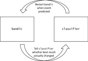
Figure 1: A high-level picture of the operation of the bwc algorithm, depicting the feedback loop between the two main subroutines, bandit and classifier.

So what prevents us from simply combining an off-the-shelf bandit algorithm with an off-the-shelf classifier? The central challenge is how to define the feedback. Let us outline several hurdles that we need to overcome here. A single false negative prediction will cause bwc to miss an event, which may result in a very high regret (since it may take the bandit algorithm a very long time to adjust). Incorrectly labeled samples may contaminate the classifier, perhaps even permanently. To generate a label for a given sample, one needs to compare the state right before the current round with the state right after, in a conclusive way. Both states are not known to the algorithm a priori, and can only be learned probabilistically via exploration. A particular challenge is to ensure that such exploration is not contaminated by events in the past rounds, as well as by events that happen soon after the current round. Moreover, this exploration is generally too expensive to perform upon negative predictions — indeed, the whole point of bwc is that in the absence of an event the bandit algorithm converges to the best arm and (essentially) keeps playing it — so the classifier receives labels only upon the positive predictions.

4.1 The meta-algorithm

We will present our algorithm in a modular way, as a meta-algorithm which uses the following two components: classifier and bandit. In each round, classifier inputs a context $x_{t}$ and outputs a “positive” or “negative” prediction of whether an event has happened in this round. Also, it may input labeled samples of the form $(x,l)$, where $x$ is a context and $l$ is a boolean label, which it uses for training. Algorithm bandit is a bandit algorithm that is tuned for the event-free runs.

As described above, we further require bandit to provide feedback to the classifier about whether the best result has actually changed. The standard bandit framework does not immediately provide us with estimates from which such feedback can be obtained. Therefore we require bandit to provide the following additional functionality: after each round $t$ of execution, it outputs a pair $(G^{+},G^{-})$ of subsets of arms; we call this pair the $t$-th round guess. The meaning of $G^{+}$ and $G^{-}$ is that they are algorithm’s estimates for, respectively, the sets of all optimal and (at least) $\epsilon_{S}$-suboptimal arms. We use $(G^{+},G^{-})$ to predict whether an event has happened between two runs of bandit. The idea is that any such event causes some arm from $G^{+}$ of the first run to migrate to $G^{-}$ of the second run. Accordingly, we generate a negative label if $G^{+}_{i}\cap G^{-}_{j}=\emptyset$, where $i$ and $j$ refers to the first and the second run, respectively (see Line 10 of Algorithm 1).

We formalize our assumptions on classifier and bandit as follows:

Definition 1.

classifier is safe for a given concept class if, given only correctly labeled samples, it never outputs a false negative. bandit is called $(L,\epsilon)$-testable, for some $L\in\mathbb{N}$ and $\epsilon\in(0,1)$, if the following holds. Consider an event-free run of bandit, and let $(G^{+},G^{-})$ be its $L$-th round guess. Then with probability at least $1-T^{-2}$, each optimal arm lies in $G^{+}$ but not in $G^{-}$, and any arm that is at least $\epsilon$-suboptimal lies in $G^{-}$ but not in $G^{+}$. 

We will discuss efficient implementations of a safe classifier and a $(L,\epsilon_{S})$-testable bandit in Sections LABEL:sec:safe and Section LABEL:sec:UCB, respectively. For bandit, we build on a standard algorithm ucb1 [bandits-ucb1]; as it turns out, making it $(L,\epsilon_{S})$-testable requires a significantly extended analysis.

For correctness, we require bandit to be $(L,\epsilon_{S})$-testable, where $\epsilon_{S}$ is the minimum shift. The performance of bandit is quantified via its event-free regret, i.e. regret on the event-free runs. Likewise, for correctness we need classifier to be safe, and we quantify its performance via the following property, termed FP-complexity, which refers to the maximum number of false positives.

Definition 2.

Given a concept class $\mathcal{F}$, the FP-complexity of classifier is the maximum possible number of false positives it can make in an online prediction game where in each round, an adversary selects a sample, classifier makes a prediction, and then (in some rounds) receives a correct label. Specifically, classifier receives a correct label if and only if the prediction is a false positive. The maximum is taken over all event oracles $f\in\mathcal{F}$ and all possible sequences of samples.

Now we are ready to present our meta-algorithm, called bwc. It runs in phases of two alternating types: odd phases are called “testing” phases, and even phases are called “adapting” phases. The first round of phase $j$ is denoted $t_{j}$. In each phase we run a fresh instance of bandit. Each testing phase lasts for $L$ rounds, where $L$ is a parameter. Each adapting phase $j$ ends as soon as classifier predicts “positive”; the round $t$ when this happens is round $t_{j+1}$. Phase $j$ is called full if it lasts at least $L$ rounds. For a full phase $j$, let $(G^{+}_{j},G^{-}_{j})$ be the $L$-th round guess in this phase. After each testing phase $j$, we generate a boolean prediction $l$ of whether there was an event in the first round thereof. Specifically, letting $i$ be the most recent full phase before phase $j$, we set $l_{t_{j}}=\texttt{false}$ if and only if $G^{+}_{i}\cap G^{-}_{j}=\emptyset$. If $l_{t_{j}}$ is false, the labeled sample $(x_{t_{j}},l_{t_{j}})$ is fed back to the classifier. Note that classifier never receives true-labeled samples. Pseudocode for bwc is given in Algorithm 1.

Disregarding the interleaved testing phases for the moment, bwc restarts bandit whenever classifier predicts “positive”, optimistically assuming that the prediction is correct. By our assumption that events cause some optimal arm to become significantly suboptimal (see Section 3), a correct prediction should result in $G^{+}_{i}\cap G^{-}_{j}\neq\emptyset$, where $i$ is a phase before the putative event, and $j$ is a phase after it. We use this condition in Line 10 of the pseudocode to generate the label. However, to ensure that the estimates $G_{i}$ and $G_{j}$ are reliable, we require that phases $i$ and $j$ are full. And to ensure that the full phases closest to a putative event are not too far from it, we interleave a full testing phase every other phase.

Algorithm 1 Meta-algorithm bwc (“Bandit with Classifier”)

1:  Given: Parameter $L$, a $(L,\epsilon_{S})$-testable bandit, and a safe classifier.

2:  for phase $j=1,2,\,\ldots\;$ do

3:     Initialize bandit. Let $t_{j}$ be current round.

4:     if $j$ is odd then

5:        {testing phase}

6:        for round $t=t_{j}\;\ldots\;t_{j}+L$ do

7:           Select arm $i_{t}$ according to bandit.

8:           Observe click w.p. $p_{t}(i_{t})$ and update bandit.

9:        Let $i$ be the most recent full phase before phase $j$.

10:        If $G^{+}_{i}\cap G^{-}_{j}=\emptyset$      {label is false}

11:             Let $l_{t_{j}}=$ false and pass training example $(x_{t_{j}},l_{t_{j}})$ to classifier.

12:     else

13:        {adapting phase}

14:        for round $t=t_{j},\,t_{j}+1,\,\ldots\;$ do

15:           Select arm $i_{t}$ according to bandit.

16:           Observe click w.p. $p_{t}(i_{t})$ and update bandit; pass context $x_{t}$ to classifier.

17:           if classifier predicts “positive” then

18:              Terminate inner for loop.

4.2 Provable guarantees

We present provable guarantees for bwc in a modular way, in terms of FP-complexity, event-free regret, and the number of events. This is the main technical result in the paper.

Theorem 1.

Consider an instance of the eventful bandit problem with number of rounds $T$, $n$ arms, $k$ events and minimum shift $\epsilon_{S}$; assume that any two events are at least $2L$ rounds apart. Consider algorithm bwc with parameter $L$ and components classifier and bandit that are, respectively, safe and $(L,\epsilon_{S})$-testable. Suppose the event-free regret of bandit is bounded from above by a concave function $R_{0}(\cdot)$. Then the regret of bwc is

$$R_{\textsc{bwc}}(T)\leq(2k+d_{\operatorname{FP}})\,R_{0}\left(\tfrac{T}{2k+d_{\operatorname{FP}}}\right)+(k+d_{\operatorname{FP}})\,R_{0}(L)+kL,$$ (1)

where $d_{\operatorname{FP}}$ is the FP-complexity of classifier.