Quadrupole collective inertia in nuclear fission: cranking approximation

Abstract

Collective mass tensor derived from the cranking approximation to the adiabatic time-dependent Hartree-Fock-Bogoliubov (ATDHFB) approach is compared with that obtained in the Gaussian Overlap Approximation (GOA) to the generator coordinate method. Illustrative calculations are carried out for one-dimensional quadrupole fission pathways in ²⁵⁶Fm. It is shown that the collective mass exhibits strong variations with the quadrupole collective coordinate. These variations are related to the changes in the intrinsic shell structure. The differences between collective inertia obtained in cranking and perturbative cranking approximations to ATDHFB, and within GOA, are discussed.

I Introduction

Microscopic understanding of nuclear collective dynamics is a long-term goal of low-energy nuclear theory. Large amplitude collective motion (LACM), as seen in fission and fusion, provides a particularly important challenge. Those phenomena can be understood in terms of many-body tunneling involving the mixing of mean fields with different symmetries. We have yet to obtain a microscopic understanding of LACM that is comparable to what we have for ground states, excited states, and response functions.

For heavy, complex nuclei, the theoretical tool of choice is the self-consistent nuclear density functional theory (DFT) [Rin80]; [Ben03]. The advantage of DFT is that, while treating the nucleus as a many-body system of fermions, it provides an avenue for identifying the essential collective degrees of freedom and provides an excellent starting point for time-dependent extensions. The time-dependent Hartree-Fock-Bogoliubov (TDHFB) theory appears, in principle, to provide a proper theoretical framework to describe the LACM. However, the main drawback of TDHFB, when applied to fission, is its inability to describe the quantum-mechanical motion under the collective barrier.

On the other hand, the adiabatic approximation to TDHFB (ATDHFB) has been successfully applied to the LACM [Bar78]; [Kri74]; [Bri76]; [Dob81]; [Gru82]; [Hee82]; [Gia80a]; [Gia80b]; [Yul99]; [Lib99]. The main assumption behind ATDHFB, well fulfilled in the context of spontaneous fission, is that the collective motion of the system is slow compared to the single-particle motion of individual nucleons [Rin80]; [Naz93c]. According to the path formulation of the fission problem [Ska08], ATDHFB provides the best framework to tackle the problem of nuclear dynamics under the barrier. Another advantage of ATDHFB is that it provides a connection between the microscopic many-body theory and phenomenological models based on collective shape variables.

The main theoretical input for an estimate of fission half-lives is collective inertia (mass tensor) and collective potential. ATDHFB provides the best framework to calculate mass tensor [Ska08]. However, in most applications, various approximations are adopted. In the commonly used cranking expression, for instance, the derivatives with respect to collective coordinates (i.e., collective momenta) are evaluated using the perturbation theory, and the Thouless-Valatin self-consistent terms yielding time-odd fields are neglected. The resulting collective masses are known to be too small [Dob81]; [Yul99]; hence it is imperative to go beyond the perturbative cranking treatment.

In the self-consistent investigations of Ref. [Yul99], based on the Gogny energy density functional, collective masses were calculated by explicitly evaluating the collective-coordinate derivatives appearing in the ATDHFB mass expression. The resulting collective mass obtained in such an approach turned out to exhibit appreciable variations along the collective path, suppressed in the perturbative cranking treatment. Furthermore, they noted that ATDHFB cranking mass could be an order of magnitude greater than the perturbative cranking mass. As noted in Ref. [Yul99], the enhanced masses obtained in the improved analysis can significantly impact the calculated fission lifetimes.

The main goal of this work is to investigate the ATDHFB cranking mass using the nuclear DFT approach with Skyrme energy functionals. The paper is organized as follows. Section II summarizes the basic ATDHFB expressions for collective inertia obtained in Ref. [Dob81]. The approximate cranking, perturbative cranking, and Gaussian Overlap Approximation (GOA) formulations are given in Sec. III. The illustrative examples of calculations are contained in Sec. IV, where the results are presented for ²⁵⁶Fm. Finally, the main results are given in Sec. V.

II ATDHFB Theory

This section contains a brief derivation of the collective mass tensor in the ATDHFB framework. Although some of the expressions are well documented in the literature [Rin80]; [Dob81], we repeat them here for the sake of completeness with particular attention paid to various approximations involved.

II.1 Summary of HFB

We begin with the HFB approach. In what follows, we use the same notation as in Ref. [Dob96fw]. The HFB formalism can be conveniently expressed in terms of the generalized density matrix, ${\cal R}$, defined as

$${\cal R}=\Bigg(\begin{array}[]{cc}\rho&\kappa\\ -\kappa^{\ast}&1-\rho^{\ast}\end{array}\Bigg)\,\,\,\,,$$ (1)

where $\rho$ and $\kappa$ are the particle and pairing densities and ${\cal R}^{2}={\cal R}$. The energy variation results in the HFB equation

$$[{\cal W},{\cal R}]=0\,\,\,,$$ (2)

which can be written as a non-linear eigenvalue problem:

$${\cal W}\left(\begin{array}[]{cc}A&B^{\ast}\\ B&A^{\ast}\end{array}\right)=\left(\begin{array}[]{cc}A&B^{\ast}\\ B&A^{\ast}\end{array}\right)\left(\begin{array}[]{cc}E&0\\ 0&-E\end{array}\right)\,\,\,,$$ (3)

where

$${\cal W}= \left(\begin{array}[]{cc}h-\lambda&\Delta\\ -\Delta^{\ast}&-h^{\ast}+\lambda\end{array}\right)\,\,\,,$$

$E$ is a diagonal matrix of quasiparticle energies $E_{\mu}$, $\lambda$ is the chemical potential, and matrices $h$ and $\Delta$ are the particle-hole and pairing mean-field potentials [Rin80], respectively.

For the sake of comparison with the commonly used BCS formalism, it is quite useful to write the HFB equations in the canonical representation. The single-particle canonical wave function $|\mu\rangle$ can be expanded in the original single-particle (harmonic oscillator) basis $|n\rangle$ as

$$|\mu\rangle=\sum_{n}~D_{n\mu}~|n\rangle,$$ (7)

where the unitary transformation $D$ is obtained by diagonalizing the density matrix $\rho$. In the canonical basis, the HFB wave function is given in a BCS-like form:

$$\breve{A}_{\mu\nu} = u_{\mu}\delta_{\mu\nu}\,\,\,,\,\,\,\breve{B}_{\mu\nu}=s_{\bar{\mu}}^{\ast}v_{\mu}\delta_{{\bar{\mu}}\nu},$$ (8)

$$u_{\mu} = u_{\bar{\mu}}=u_{\mu}^{\ast}\,\,\,,\,\,\,v_{\mu}=v_{\bar{\mu}}=v_{\mu}^{\ast},$$ (9)

where the phase $s_{\mu}$, for the time-even quasiparticle vacuum considered here, is defined through the time-inversion of the single-particle states

$$\hat{T}|\mu\rangle=s_{\mu}|\bar{\mu}\rangle\,\,\,,\,\,\,s_{\bar{\mu}}=-s_{\mu}\,\,\,.$$ (10)

In Eq. (8) and in the following, the quantities in the canonical basis are denoted by symbols with breve accents [Dob96fw].

The HFB energy matrix $\breve{E}$ in the canonical basis is non-diagonal and is given by

$$\breve{E}_{\mu\nu}=\xi^{+}_{\mu\nu}~(\breve{h}-\lambda)_{\mu\nu}-\eta^{+}_{\mu\nu}~\breve{\Delta}_{\mu\bar{\nu}}~s_{\bar{\nu}}^{\ast}\,\,\,,$$ (11)

where

$$\eta^{\pm}_{\mu\nu}=u_{\mu}v_{\nu}\pm u_{\nu}v_{\mu}\quad{\rm and}\quad\xi^{\pm}_{\mu\nu}=u_{\mu}u_{\nu}\mp v_{\mu}v_{\nu}\,.$$ (12)

The diagonal matrix elements of the matrix $\breve{E}_{\mu\nu}$ can be written as [Rin80]; [Dob96fw]:

$$\breve{E}_{\mu}\equiv\breve{E}_{\mu\mu}=\sqrt{(\breve{h}_{\mu\mu}-\lambda)^{2}+\breve{\Delta}_{\mu\bar{\mu}}^{2}}\,\,\,.$$ (13)

Even though the above equation resembles the BCS expression for quasiparticle energy, it involves $\breve{h}_{\mu\mu}$ and $\breve{\Delta}_{\mu\bar{\mu}}$, which are respectively obtained by transforming the HFB particle-hole and the pairing fields to the canonical basis via the transformation (7). It is only in the BCS approximation that these quantities can be associated with single-particle energies and the pairing gap.

II.2 Summary of ATDHFB

The ATDHFB approach is an approximation to the time-dependent HFB theory, wherein it is assumed that the collective velocity of the system is small compared to the average single-particle velocity of the nucleons. The generalized HFB density matrix is expanded around the quasi-stationary HFB solution ${\cal R}_{0}$ up to quadratic terms in the collective momentum:

$${\cal R}={\cal R}_{0}+{\cal R}_{1}+{\cal R}_{2}\,,$$ (14)

with ${\cal R}_{1}$ being time-odd and ${\cal R}_{0}$ and ${\cal R}_{2}$ time-even densities. The corresponding expansion for the HFB Hamiltonian reads

$${\cal W}={\cal W}_{0}+{\cal W}_{1}+{\cal W}_{2}.$$ (15)

Employing the density expansion (14), the HFB energy can be separated into the collective kinetic and the potential parts. In terms of the density expansion (14), the kinetic energy is given by

$${\cal K} = \frac{1}{2}{\rm Tr}({\cal W}_{0}{\cal R}_{2})+\frac{1}{4}{\rm Tr}({\cal W}_{1}{\cal R}_{1})$$ (16)

$$= \frac{i}{4}{\rm Tr}\left({\dot{\cal R}_{0}}[{\cal R}_{0},{\cal R}_{1}]\right)-\frac{1}{2}\left([{\cal R}_{2},{\cal R}_{0}][{\cal W}_{0},{\cal R}_{0}]\right).$$

In the usual ATDHFB treatment, the second term involving ${\cal R}_{2}$ is neglected, and the kinetic energy can be written in the familiar form:

$${\cal K}=\frac{1}{2}{\dot{q}}^{2}{\cal M}\,,$$ (17)

where the collective mass is given by

$${\cal M} = \frac{i}{2{\dot{q}}^{2}}{\rm Tr}\biggr({\dot{\cal R}_{0}}[{\cal R}_{0},{\cal R}_{1}]\biggr)$$ (18)

$$= \frac{i}{2{\dot{q}}}{\rm Tr}\biggr(\frac{\partial{\cal R}_{0}}{\partial q}[{\cal R}_{0},{\cal R}_{1}]\biggr).$$ (19)

The trace in the above expression can easily be evaluated in the quasiparticle basis. To this end, one can utilize the ATDHFB equation [Bar78]; [Kri74]; [Bri76]; [Dob81]

$$i{\dot{\cal R}_{0}}=[{\cal W}_{0},{\cal R}_{1}]+[{\cal W}_{1},{\cal R}_{0}]\,.$$ (20)

In the quasiparticle basis, the matrices ${\cal R}_{0},{\cal W}_{0},{\cal W}_{1},{\cal R}_{1}$, and ${\dot{\cal R}_{0}}$ are represented by the matrices ${\cal G},{\cal E}_{0},{\cal E}_{1},{\cal Z}$, and ${\cal F}$, respectively:

$${\cal R}_{0} = {\cal A}{\cal G}{\cal A}^{\dagger}\,,$$ (21)

$${\cal W}_{0} = {\cal A}{\cal E}_{0}{\cal A}^{\dagger}\,,$$ (22)

$${\cal W}_{1} = {\cal A}{\cal E}_{1}{\cal A}^{\dagger}\,,$$ (23)

$${\cal R}_{1} = {\cal A}{\cal Z}{\cal A}^{\dagger}\,,$$ (24)

$${\dot{\cal R}_{0}} = {\cal A}{\cal F}{\cal A}^{\dagger}\,,$$ (25)

where

$${\cal A}=\left(\begin{array}[]{cc}A&B^{\ast}\\ B&A^{\ast}\end{array}\right)$$ (26)

is the matrix of the Bogolyubov transformation, and

$${\cal G}=\left(\begin{array}[]{cc}0&0\\ 0&1\end{array}\right)\quad,{\rm}\quad{\cal E}_{0}=\left(\begin{array}[]{cc}E&0\\ 0&-E\end{array}\right).$$ (27)

ATDHFB equation (20) can now be written in the quasiparticle basis as

$$i{\cal F}=[{\cal E}_{0},{\cal Z}]+[{\cal E}_{1}\,,{\cal G}]\,.$$ (28)

This $2\times 2$ matrix equation is, in fact, equivalent [Dob81] to the following equation,

$$iF=E~Z+Z~E+E_{1}\,\,\,,$$ (29)

where the antisymmetric matrices $F$, $Z$, and $E_{1}$ are related to ${\cal F}$, ${\cal Z}$, and ${\cal E}_{1}$:

$${\cal F}=\left(\begin{array}[]{cc}0&F\\ -F^{\ast}&0\end{array}\right)\quad \quad{\cal Z}=\left(\begin{array}[]{cc}0&Z\\ -Z^{\ast}&0\end{array}\right)$$ ,

$${}[{\cal E}_{1}\,,{\cal G}] = \left(\begin{array}[]{cc}0&E_{1}\\ -E_{1}^{\ast}&0\end{array}\right).$$

In the case of several collective coordinates $\{q_{i}\}$, the ATDHFB equation (20) must be solved for each coordinate,

$$i{\dot{q}}_{i}\frac{\partial{\cal R}_{0}}{\partial q_{i}}=[{\cal W}_{0},{\cal R}_{1}^{i}]+[{\cal W}_{1}^{i},{\cal R}_{0}]\,,$$ (38)

and the collective mass tensor becomes:

$${\cal M}_{ij}=\frac{i}{2\dot{q}_{j}}{\rm Tr}\biggr(\frac{\partial{\cal R}_{0}}{\partial q_{i}}[{\cal R}_{0},{\cal R}_{1}^{j}]\biggr).$$ (39)

Then, in terms of the corresponding matrices $F^{i}$ and $Z^{j}$, the collective mass tensor is given by

$${\cal M}_{ij}=\frac{i}{2{\dot{q}_{i}}{\dot{q}_{j}}}{\rm Tr}\biggr(F^{i\ast}Z^{j}-F^{i}Z^{j\ast}\biggr).$$ (40)

The expression (40) for the mass tensor contains the matrix $Z^{i}$, which is associated with time-odd density matrix ${\cal R}_{1}^{i}$ and can, in principle, be obtained by solving the HFB equations with time-odd fields. The time-odd fields have been incorporated in mass-tensor calculations only in a limited number of cases. For instance, in Ref. [Gia80b], time-odd fields have been included in the HF study with a constraint of cylindrical symmetry. The time-odd fields have also been incorporated in the HFB study in an approximate iterative scheme with the collective path based on the Woods-Saxon potential [Dob81].

III Approximations to ATDHFB

This section contains the summary of various commonly used approximations to the exact ATDHFB expression (40).

III.1 Cranking approximation

In most of the studies, the time-odd interaction matrix $E_{1}$ appearing in Eq. (29) is neglected. In the following, this approximation will be referred to as the cranking approximation (ATDHFB-C). In the absence of the term involving $E_{1}$, the $Z$-matrix can be easily obtained in the quasiparticle basis from the equation:

$$-iF^{i}_{\mu\nu}=(E_{\mu}+E_{\nu}){Z}^{i}_{\mu\nu}\,\,\,$$ (41)

and the collective cranking mass tensor is given by:

$${\cal M}^{C}_{ij}=\frac{1}{2{\dot{q}_{i}}{\dot{q}_{j}}}\sum_{\mu\nu}\frac{\left(F^{i\ast}_{\mu\nu}F^{j}_{\mu\nu}+F^{i}_{\mu\nu}F^{j\ast}_{\mu\nu}\right)}{E_{\mu}+E_{\nu}}.$$ (42)

It should be noted that Eq. (41) is diagonal in the quasiparticle basis and not in the canonical basis. The essential input to the ATDHFB-C mass tensor (42) is the matrix $F$. In the following, $F$ is evaluated in both canonical and quasiparticle basis.

III.1.1 Canonical basis

To begin with, Eq. (25) can be written explicitly in terms of the HFB eigenvectors:

$${\dot{\cal R}_{0}}={\dot{q}}\frac{\partial}{\partial q}\Bigg(\begin{array}[]{cc}\rho_{0}&\kappa_{0}\\ -\kappa_{0}^{\ast}&1-\rho_{0}^{\ast}\end{array}\Bigg)=$$

$$=\left(\begin{array}[]{cc}AFB^{T}-B^{\ast}F^{\ast}A^{\dagger}&AFA^{T}-B^{\ast}F^{\ast}B^{\dagger}\\ BFB^{T}-A^{\ast}F^{\ast}A^{\dagger}&BFA^{T}-A^{\ast}F^{\ast}B^{\dagger}\end{array}\right).$$

Evaluating the matrix elements of (III.1.1) in the canonical basis, we obtain

$$\breve{F}^{i}_{\mu\bar{\nu}}=\frac{s_{\bar{\nu}}}{(u_{\mu}v_{\nu}+v_{\mu}u_{\nu})}{\dot{q}_{i}}\biggr(\frac{\partial\rho_{0}}{\partial q_{i}}\biggr)_{\mu\nu}\,.$$ (49)

By differentiating the HFB equation $[{\cal W}_{0},{\cal R}_{0}]=0$ with respect to $q_{i}$, the derivative of the density matrix in (49) can be expressed in terms of the derivatives of the particle-hole and the pairing mean-fields. The resulting 2$\times$2 matrix equation is

$$\bigg[{\cal A}^{\dagger}{\dot{q}_{i}}\frac{\partial{\cal W}_{0}}{\partial q_{i}}{\cal A},{\cal G}\bigg]+\bigg[{\cal E}_{0},{\cal F}\bigg]=0.$$ (50)

By employing the properties of $h$ and $\Delta$ with respect to time reversal, we obtain

$$\bigg(\frac{\partial h^{\ast}}{\partial q_{i}}\bigg)_{\mu\nu} = s^{\ast}_{\mu}s_{\nu}\bigg(\frac{\partial h}{\partial q_{i}}\bigg)_{\bar{\mu}\bar{\nu}}\,\,\,,$$ (51)

$$\bigg(\frac{\partial\Delta^{\ast}}{\partial q_{i}}\bigg)_{\mu\nu} = s^{\ast}_{\mu}s^{\ast}_{\nu}\bigg(\frac{\partial\Delta}{\partial q_{i}}\bigg)_{\bar{\mu}\bar{\nu}},$$ (52)

and by approximating the HFB energy matrix in the canonical basis by its diagonal matrix elements,

$$\breve{E}_{\mu\nu}\approx\delta_{\mu\nu}\breve{E}_{\mu},$$ (53)

one arrives at an approximate “BCS-equivalent” expression for the matrix elements of $F$ in the canonical basis:

$$\breve{F}^{i}_{\mu\nu}\approx\frac{-\dot{q}_{i}}{\breve{E}_{\mu}+\breve{E}_{\nu}}\left[s_{\nu}\eta^{+}_{\mu\nu}(\breve{h}^{i}-\lambda^{i})_{\mu\bar{\nu}}+\xi^{+}_{\mu\nu}(\breve{\Delta}^{i})_{\mu\nu}\right],$$ (54)

where $x^{i}\equiv\partial x/\partial q_{i}$ with $x=\breve{h}$, $\breve{\Delta}$, or $\lambda$. In the following, the results obtained by using this approximation will be called ATDHFB-C^c.

Using relations (53) and (54), the collective mass tensor (42) can now be expressed in terms of the derivatives of the mean-field potentials with respect to the collective coordinates $q_{i}$ and BCS-like quasiparticle energies (13),

$${\cal M}^{C^{\rm c}}_{ij}\approx\frac{1}{2{\dot{q}_{i}}{\dot{q}_{j}}}\sum_{\mu\nu}\frac{\left(\breve{F}^{i\ast}_{\mu\nu}\breve{F}^{j}_{\mu\nu}+\breve{F}^{i}_{\mu\nu}\breve{F}^{j\ast}_{\mu\nu}\right)}{\breve{E}_{\mu}+\breve{E}_{\nu}}.$$ (55)

In the one-dimensional case, the resulting expression agrees with that of Ref. [Yul99].

III.1.2 Quasiparticle basis

In order to obtain the expression for matrix $F$ in the quasiparticle basis, we invert Eq. (25) and write the matrix expression for ${\cal F}={\cal A}^{\dagger}{\dot{\cal R}}_{0}{\cal A}$

$${\cal F}=\left(\begin{array}[]{cc}A^{\dagger}{\dot{\rho}}_{0}A+A^{\dagger}{\dot{\kappa}}_{0}B-B^{\dagger}{\dot{\kappa}}_{0}^{\ast}A-B^{\dagger}{\dot{\rho}}_{0}^{\ast}B&\,\,\,A^{\dagger}{\dot{\rho}}_{0}B^{\ast}+A^{\dagger}{\dot{\kappa}}_{0}A^{\ast}-B^{\dagger}{\dot{\kappa}}_{0}^{\ast}B^{\ast}-B^{\dagger}{\dot{\rho}}_{0}^{\ast}A^{\ast}\\ B^{T}{\dot{\rho}}_{0}A+B^{T}{\dot{\kappa}}_{0}B-A^{T}{\dot{\kappa}}_{0}^{\ast}A-A^{T}{\dot{\rho}}_{0}^{\ast}B&\,\,\,B^{T}{\dot{\rho}}_{0}B^{\ast}+B^{T}{\dot{\kappa}}_{0}A^{\ast}-A^{T}{\dot{\kappa}}_{0}^{\ast}B^{\ast}-A^{T}{\dot{\rho}}_{0}^{\ast}A^{\ast}\end{array}\right)\,\,\,.$$ (56)

Elements (1,1) and (2,2) of ${\cal F}$ vanish because ${\cal R}_{0}$ is projective, ${\cal R}_{0}^{2}={\cal R}_{0}$. Equating the above expression with Eq. (II.2), we obtain

$$-F^{\ast}=B^{T}{\dot{\rho}}_{0}A+B^{T}{\dot{\kappa}}_{0}B-A^{T}{\dot{\kappa}}_{0}^{\ast}A-A^{T}{\dot{\rho}}_{0}^{\ast}B\,\,\,.$$ (57)

In the following, we evaluate the above expression in the simplex basis, as the mean-field analysis has been performed by imposing this symmetry. In this basis, the HFB wave function has the following structure

$$B=\left(\begin{array}[]{cc}B_{+}&0\\ 0&B_{-}\end{array}\right)\,\,\,{\rm and}\,\,\,A=\left(\begin{array}[]{cc}0&A_{+}\\ A_{-}&0\end{array}\right)\,\,.$$ (58)

The density matrices acquire the following forms in the simplex basis

$$\rho=\left(\begin{array}[]{cc}B_{+}^{\ast}B_{+}^{T}&0\\ 0&B_{-}^{\ast}B_{-}^{T}\end{array}\right) = \left(\begin{array}[]{cc}\rho_{+}&0\\ 0&\rho_{-}\end{array}\right)\,\,\,,$$

$$\kappa=\left(\begin{array}[]{cc}0&B_{+}^{\ast}A_{-}^{T}\\ B_{-}^{\ast}A_{+}^{T}&0\end{array}\right) = \left(\begin{array}[]{cc}0&\kappa_{+}\\ \kappa_{-}&0\end{array}\right)\,\,\,.$$

The simplex structure of various terms in Eq. (57) is given by

$$B^{T}{\dot{\rho}}_{0}A = \left(\begin{array}[]{cc}0&B^{T}_{+}{\dot{\rho}}_{0+}A_{+}\\ B^{T}_{-}{\dot{\rho}}_{0-}A_{-}&0\end{array}\right)\,\,\,,$$

$$A^{T}{\dot{\rho}}^{\ast}_{0}B = \left(\begin{array}[]{cc}0&A^{T}_{-}{\dot{\rho}}_{0-}^{\ast}B_{-}\\ A^{T}_{+}{\dot{\rho}}_{0^{+}}^{\ast}B_{+}&0\end{array}\right)\,\,\,,$$

$$B^{T}{\dot{\kappa}}_{0}B = \left(\begin{array}[]{cc}0&B^{T}_{+}{\dot{\kappa}}_{0+}B_{-}\\ B^{T}_{-}{\dot{\kappa}}_{0-}B_{+}&0\end{array}\right)\,\,\,,$$

$$A^{T}{\dot{\kappa}}_{0}^{\ast}A = \left(\begin{array}[]{cc}0&A^{T}_{-}{\dot{\kappa}}_{0-}^{\ast}A_{+}\\ A^{T}_{+}{\dot{\kappa}}_{0+}^{\ast}A_{-}&0\end{array}\right)\,\,\,.$$

This yields:

$$-F^{\ast} = \left(\begin{array}[]{cc}0&F_{+}\\ F_{-}&0\end{array}\right),$$

where

$$F_{+} = B^{T}_{+}{\dot{\rho}}_{0+}A_{+}-A^{T}_{-}{\dot{\rho}}_{0-}^{\ast}B_{-}$$ (84)

$$+ B^{T}_{+}{\dot{\kappa}}_{0+}B_{-}-A^{T}_{-}{\dot{\kappa}}_{0-}^{\ast}A_{+},$$

$$F_{-} = B^{T}_{-}{\dot{\rho}}_{0-}A_{-}-A^{T}_{+}{\dot{\rho}}_{0+}^{\ast}B_{+}$$ (85)

$$+ B^{T}_{-}{\dot{\kappa}}_{0-}B_{+}-A^{T}_{+}{\dot{\kappa}}_{0+}^{\ast}A_{-}.$$

Since $F$ is antisymmetric, we have obviously $F_{+}^{T}=-F_{-}$, which is fulfilled explicitly provided $\kappa_{+}^{T}=-\kappa_{-}$.

III.1.3 Calculation of derivatives

The collective mass involves either derivatives of the density matrices or the mean-field potentials. It should be stressed that these derivatives must be calculated in the original single-particle basis $|n\rangle$ as the canonical basis (7) varies with $\{q_{i}\}$. In the following, we show how to evaluate the collective derivatives in the one-dimensional case of single collective coordinate, the quadrupole deformation $q$. To this end, we approximate the derivative of the density operator $\rho$ or $\kappa$ at a deformation point $q=q_{0}$ by means of the Lagrange three-point formula for unequally spaced points $q_{0}-\delta q$, $q_{0}$, and $q_{0}+\delta q^{\prime}$ [Gia80b]; [Yul99]; [Abr70]:

$$\biggr(\frac{\partial\rho}{\partial q}\biggr)_{q=q_{0}} \approx \frac{-\delta q^{\prime}}{\delta q(\delta q+\delta q^{\prime})}\rho(q_{0}-\delta q)+\frac{\delta q-\delta q^{\prime}}{\delta q\,\delta q^{\prime}}\rho(q_{0})$$ (86)

$$+\frac{\delta q}{\delta q^{\prime}(\delta q+\delta q^{\prime})}\rho(q_{0}+\delta q^{\prime}).$$

The reason for the use of unequally spaced grid in Eq. (86) is purely numerical: the constrained HFB equations cannot be precisely solved at a requested deformation point $q$.

The corresponding matrix element in the canonical basis can be expressed through the matrices $D_{n\nu}$ of the canonical transformation (7):

$$\bigg(\frac{\partial\rho}{\partial q}\bigg)_{\mu\nu}\!\!\! \approx \!\!\!\frac{-\delta q^{\prime}}{\delta q(\delta q+\delta q^{\prime})}\sum_{n_{1}n_{2}}D^{\ast}_{n_{1}\mu}(\rho(q_{0}-\delta q))_{n_{1}n_{2}}D_{n_{2}\nu}$$ (87)

$$+ \!\!\!\frac{\delta q-\delta q^{\prime}}{\delta q\,\delta q^{\prime}}v^{2}_{\mu}\delta_{\mu\nu}$$

$$+ \!\!\!\frac{\delta q}{\delta q^{\prime}(\delta q+\delta q^{\prime})}\sum_{n_{1}n_{2}}D^{\ast}_{n_{1}\mu}(\rho(q_{0}+\delta q^{\prime}))_{n_{1}n_{2}}D_{n_{2}\nu}.$$

It should be noted that the canonical matrix $D_{n\nu}$ in the above expression corresponds to the deformation point, $q_{0}$, at which the mass is evaluated. Furthermore, as mentioned above, the density matrices at the three deformation points in (86) need to be calculated using the single-particle basis $|n\rangle$ with the same basis deformation.

III.2 Perturbative cranking approximation

The perturbative cranking approximation (ATDHFB-C^p) has been widely used for the evaluation of the collective mass tensor. In this approximation, apart from neglecting the time-odd interaction terms in the ATDHFB equation and off-diagonal matrix elements of the HFB energy matrix (53), the derivatives are not evaluated explicitly but are obtained using a perturbative approach. A complete description of the perturbative cranking model as applied to the nuclear fission process can be found in Refs. [Bel59]; [Bes61]; [Nil69]; [Sob69]; [Bra72].

The perturbative cranking expression for the mass tensor is obtained by approximating the mean-field derivatives in Eq. (49) by canonical-basis expressions. For instance, the matrix element of $h^{i}$ can be approximated by

$$\langle\nu|h^{i}|\mu\rangle\approx(\breve{h}_{\mu}-\breve{h}_{\nu})\langle\nu|\partial_{i}\mu\rangle,$$ (88)

for $\mu\neq\nu$ which, together with

$$\langle\mu|{h}^{i}|\mu\rangle\approx\partial_{i}\breve{h}_{\mu} = \breve{h}^{i}_{\mu},$$ (89)

$$\partial_{i}\breve{\Delta}_{\mu} = \breve{\Delta}^{i}_{\mu},$$ (90)

for $\breve{h}_{\mu}\equiv\breve{h}_{\mu\mu}$ and $\breve{\Delta}_{\mu}\equiv-\breve{\Delta}_{\mu\bar{\mu}}s_{\bar{\mu}}^{*}$, leads to the following expression for the cranking mass tensor

$${\cal M}^{C^{\rm p}}_{ij}\approx\sum_{\mu\neq\nu}\frac{\langle\mu|h^{i}|\nu\rangle\langle\nu|h^{j}|\mu\rangle}{(\breve{h}_{\mu}-\breve{h}_{\nu})^{2}(\breve{E}_{\mu}+\breve{E}_{\nu})}(\eta^{-}_{\mu\nu})^{2}+\sum_{\mu}\frac{F_{\mu}^{i}F_{\mu}^{j}}{2\breve{E}_{\mu}}$$ (91)

where

$$F_{\mu}^{i}\equiv F_{\mu\bar{\mu}}^{i}=-\frac{1}{2\breve{E}_{\mu}^{2}}[\breve{\Delta}_{\mu}(\breve{h}_{\mu}^{i}-\lambda^{i})-(\breve{h}_{\mu}-\lambda)\breve{\Delta}_{\mu}^{i}].$$ (92)

Assuming a weak state dependence of $\breve{\Delta}_{\mu}$ [Sie03], neglecting the derivatives of $\Delta$ and $\lambda$ [Bra72], and using the identity

$$\frac{\eta^{-}_{\mu\nu}}{\eta^{+}_{\mu\nu}}=\frac{(\breve{h}_{\mu}-\lambda)\breve{\Delta}_{\nu}-(\breve{h}_{\nu}-\lambda)\breve{\Delta}_{\mu}}{\breve{E}_{\mu}\breve{\Delta}_{\nu}+\breve{E}_{\nu}\breve{\Delta}_{\mu}},$$ (93)

one arrives at the following perturbative cranking mass tensor:

$${\cal M}^{C^{\rm p}}_{ij}\approx\sum_{\mu\nu}\frac{\langle\mu|h^{i}|\nu\rangle\langle\nu|h^{j}|\mu\rangle}{(\breve{E}_{\mu}+\breve{E}_{\nu})^{3}}(\eta^{+}_{\mu\nu})^{2},$$ (94)

where the sums run over the whole set of canonical states. This expression resembles the standard cranking expression for the collective mass tensor [Bel59]; [Bes61]; [Sob69]; [Bra72] originally derived for a phenomenological mean field $h$.

III.3 Gaussian overlap approximation

To compare cranking expressions with those obtained within the GOA, it is convenient to introduce the $\cal S$ matrices [Sta89a]:

$${\cal S}_{ij}^{(K)}=\sum_{\mu,\nu}\frac{\langle\mu|h^{i}|\nu\rangle\langle\nu|h^{j}|\mu\rangle}{(\breve{E}_{\mu}+\breve{E}_{\nu})^{K}}(\eta^{+}_{\mu\nu})^{2}.$$ (95)

It is immediately seen that for the mass tensor of Eq. (94) one has ${\cal M}^{C}={\cal S}^{(3)}$. In the case of GOA, also assuming weak state dependence of pairing and neglecting the derivatives of $\lambda$ and $\Delta_{\mu\bar{\mu}}$, one obtains [Goz85]; [Sta89a]

$${\cal M}^{\rm GOA}={\cal S}^{(2)}\left[{\cal S}^{(1)}\right]^{-1}{\cal S}^{(2)}.$$ (96)

Evaluating the matrix elements of $h^{i}$ entering Eq. (95) perturbatively, one can express ${\cal S}$ explicitly through the matrix elements of the constraining field operators $\hat{Q}_{i}$:

$${\cal S}^{(K)}=\frac{1}{4}\left[{M}^{(1)}\right]^{-1}{M}^{(K)}\left[{M}^{(1)}\right]^{-1},$$ (97)

where the energy-weighted moments ${M}^{(K)}$ are given by

$$M^{(K)}_{ij}=\sum_{\mu\nu}\frac{\langle\mu|\hat{Q}_{i}|\nu\rangle\langle\nu|\hat{Q}_{j}^{\dagger}|\mu\rangle}{(\breve{E}_{\mu}+\breve{E}_{\nu})^{K}}(\eta_{\mu\nu}^{+})^{2}.$$ (98)

III.4 Treatment of proton and neutron contributions

The above expressions for the mass tensor are valid for one kind of fermions only. In the case of the cranking approximation, the total mass tensor is a sum of neutron and proton contributions:

$${\cal M}^{C}_{\rm total}={\cal M}^{C}_{\rm n}+{\cal M}^{C}_{\rm p}.$$ (99)

In the GOA, however, the total inverse inertia $({\cal M}^{\rm GOA}_{\rm total})^{-1}$ for a composite system is given as a sum of proton and neutron inverse covariant inertia tensors [Goz85]:

$$({\cal M}^{\rm GOA}_{\rm total})^{-1}=({\cal M}^{\rm GOA}_{n})^{-1}+({\cal M}^{\rm GOA}_{p})^{-1}.$$ (100)

IV Results

The illustrative calculations were performed for the nucleus ²⁵⁶Fm by using the SkM^∗ energy density functional [Bar82] in the particle-hole (ph) channel. In the particle-particle (pp) channel we employed the density-dependent pairing interaction in the mixed variant of Refs. [Dob01c]; [Dob02c]:

$$V_{\tau}(\vec{r})=V_{\tau 0}\left(1-\rho(\vec{r})/2\rho_{0}\right)\delta(\vec{r})\,,$$ (101)

where $\tau=n,p$ and $\rho_{0}=0.16\,$fm^-1. To test the accuracy of various approximations, we carried out both HF+BCS and HFB calculations. The pairing interaction strengths, which were adjusted to reproduce the neutron and proton ground-state pairing gaps in ²⁵²Fm, are (in $\mbox{MeV fm}^{3}$):

$$V_{n0}=-372.0\,,\quad V_{p0}=-438.0\,.$$ (102)

The fission pathways were studied in the previous Ref. [Sta09] using the SkM^∗-HF-BCS approach with the seniority pairing interaction. It has been found that the SkM^∗ energy density functional favors the asymmetric fission pathway in ²⁵⁶Fm, and our HFB results are consistent with this result. The one-dimensional collective pathway, determined by the axial quadrupole moment $q=Q_{20}$, was obtained by means of the HFB solver HFODD [Dob09e].

Figure 1: (Color online) The quadrupole mass parameter (top: total; middle: neutron contribution; bottom: proton contribution) along the fission pathway of ²⁵⁶Fm calculated in SkM^∗+HF+BCS as a function of the mass quadrupole moment. The ATDBCS-C results (triangles) are compared with those obtained in the perturbative cranking approximation (ATDBCS-C^p, circles) and Gaussian overlap approximation (ATDBCS^GOA, diamonds). See text for details.

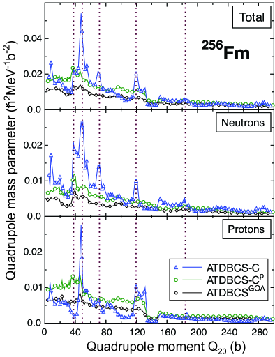
Using the self-consistent solutions along the fission pathway, we calculate the collective quadrupole mass parameter using various approximations described in Sec. III. First, we discuss results obtained within the HF+BCS formalism (dubbed ATDBCS). Figure 1 compares the results of the non-perturbative cranking approach (ATDBCS-C) with the perturbative cranking approximation (ATDBCS-C^p) and Gaussian overlap approximation (ATDBCS^GOA). In ATDBCS-C the derivatives of the density matrices and the mean-field potentials have been obtained using the Lagrange formula, which requires the knowledge of self-consistent solutions in several neighboring deformation points. We have evaluated the density matrices for quadrupole deformations ranging from $Q_{20}$= 0 to 320 b in steps of 1 b. The derivatives were obtained by using the 3-point Lagrange formula (87), and also the 5-point Lagrange formula [Abr70]. The results for collective mass obtained with 3-point and 5-point expressions differ only in the third decimal place; hence, in the following, we shall stick to the 3-point Lagrange formula. It needs to be stressed that – in order to guarantee consistent labeling of canonical states – the underlying single-particle basis should be identical for all three points in Eq. (87) involved in the derivative evaluation. This has been achieved by performing HF+BCS calculations using the same basis deformation for all neighboring points.

As seen in Fig. 1, the total ATDBCS-C mass exhibits a rather irregular behavior characterized by the presence of several sharp maxima. Some of these peak-like structures, although considerably suppressed, also show up in ATDBCS-C^p and ATDBCS^GOA.

Figure 2: (Color online) Total HF+BCS energy $E_{\rm tot}$ (top), pairing energies $E_{\rm pp}$ (total, proton, and neutron; middle), and the HF energy $E_{\rm ph}$ (bottom) calculated along the fission pathway for ²⁵⁶Fm. The borders between different self-consistent configurations are marked by vertical solid lines. The dotted lines mark positions of peaks in the collective ATDBCS-C mass parameter of Fig. 1.

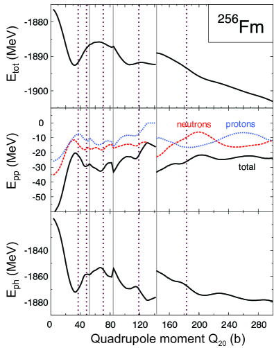
To unravel the origin of the peak structures in the collective mass, the total energy of ²⁵⁶Fm is depicted in Fig. 2, together with corresponding pairing-energy $(E_{\rm pp})$ and HF energy $(E_{\rm ph})$ contributions. The one-dimensional total energy curve shows several discontinuities due to intersections of close-lying energy sheets (surfaces) with very different mean fields. The corresponding pathways can in fact be well separated when studied in more than one dimension of the collective manifold [Sta09]. The diabatic jumps between various energy sheets have been disregarded when computing the collective inertia shown in Fig. 1. Indeed, in such cases the adiabatic theory is unable to provide a meaningful result for the collective mass.

There are also configuration changes within each pathway. Because of pairing correlations, these changes are adiabatic in character [Neg89a]; [Naz93c]. Still, they manifest themselves in the collective inertias through the appearance of peaks [Gri71a]; [Sch80a]; [Arv88]. Figures 1 and 2 nicely illustrate this point: the peaks in the collective ATDBCS-C mass parameter appear in the regions of large local variations in $E_{\rm pp}$ and $E_{\rm ph}$ that are indicative of changes in the shell structure with elongation. (We note that the local variations in the total energy are much weaker than those in pairing and HF energies, due to the well-known anticorrelation between pairing and HF energies, clearly seen in Fig. 2.)

Two general conclusions can be drawn from the results of Fig. 1. First, the ATDBCS-C^p and ATDBCS^GOA inertia show fairly similar behavior, with the ATDBCS-C^p mass being systematically larger. Second, the exact treatment of derivative terms in ATDBCS-C gives rise to less adiabatic behavior in the corresponding collective mass.

The results obtained within the HFB framework are presented in Fig. 3. The results obtained in the canonical approximation ATDHFB-C^c (55), perturbative treatment of derivatives ATDHFB-C^p (91), and ATDHFB^GOA (96) were obtained by using the canonical HFB wave functions and employing the diagonal (“equivalent BCS”) ansatz. The ATDHFB-C calculations (42) were carried out in the full quasiparticle basis.

Figure 3: (Color online) The quadrupole mass parameter (top: total; middle: neutron contribution; bottom: proton contribution) along the fission pathway of ²⁵⁶Fm calculated in SkM^∗+HFB as a function of the mass quadrupole moment. The ATDHFB-C results (triangles) are compared with those obtained in the canonical approximation (ATDHFB-C^c, squares), perturbative cranking approximation (ATDHFB-C^p, dots), and Gaussian overlap approximation (ATDHFB^GOA, diamonds). See text for details.

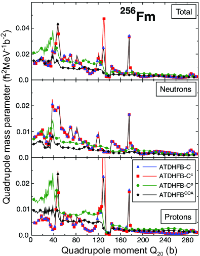
The most interesting finding is that the collective mass in ATDHFB-C is very close to that obtained in ATDHFB-C^c. Similar to the HF-BCS case, the ATDHFB-C^p and ATDHFB^GOA results follow each other with the ATDHFB-C^p mass being systematically larger. Again, the exact treatment of derivatives gives rise to less adiabatic behavior of collective mass that manifests itself through the presence of peaks.

In Ref. [Yul99], the quadrupole collective mass was evaluated in the canonical basis and exhibited a singular behavior at certain deformation points. The primary reason for this singularity is due to the pairing collapse at certain deformations that results in unphysical phase transition and the presence of unavoided level crossings. In our work, the peak structures are present at nonzero pairing and are related to the shell structure changes along the fission pathways.

In order to highlight the differences between HFB and BCS treatments, Fig. 4 shows the quadrupole masses obtained in these approaches in the region of the ground-state minimum and the inner fission barrier of ²⁵⁶Fm ($Q_{20}\in[20,100]$). This region plays a crucial role in the evaluation of fission half-lives. It is evident from Fig. 4 that the non-perturbative cranking masses ATDBCS-C and ATDHFB-C have very similar behavior. On the other hand, the masses calculated in the perturbative approximations, ATDBCS-C^p and ATDHFB-C^p, are quite different for $Q_{20}<40$. Furthermore, in this region, the perturbative masses appear to be quite large as compared to the cranking values.

Figure 4: (Color online) Similar as in Fig. 3 except for ATDHFB-C (filled triangles), ATDBCS-C (open triangles), ATDHFB-C^p (dots), and ATDBCS-C^p (circles) in the narrower region of 20 b $\leq$$Q_{20}$$\leq$100 b.

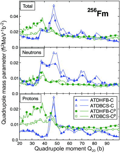
The high-frequency fluctuations of collective mass can be traced back to the imperfect numerical convergence of HFB calculations. In the present work, we assumed the accuracy of 0.001 MeV for the total energy. This results in an uncertainty of about 0.002 $\hbar^{2}$/(MeV b²) in the collective inertia. If required, the precision of these calculations can be increased at the expense of an appreciably higher CPU time.

V Summary

The primary motivation of the present work has been to assess various approximations to the collective mass for fission. The collective mass plays a crucial role in determining the adiabatic collective motion of the nucleus and strongly impacts predicted half-lives. In the majority of previous studies, cranking approximation to collective mass has been employed, in which the time-odd fields are ignored and the collective momenta (i.e., derivatives with respect to collective coordinates) needed in the evaluation of the ATDHFB mass are calculated using the perturbation theory.

In our study, we performed the full ATDHFB cranking treatment of quadrupole inertia. The numerical evaluation of the derivatives appearing in ATDHFB mass expression poses a serious computational challenge as the accurate self-consistent HFB solutions need to be obtained at several neighboring points around every deformation along the fission pathway. By comparing three- and five-point approximations, we conclude that the three-point Lagrange formula provides a reasonable description of collective derivatives.

The main conclusions of this work can be summarized as follows.

• The collective masses obtained in non-perturbative treatment of derivatives show more variations due to shell structure changes along the fission path as compared to the perturbative approximation and GOA.

• The collective mass in full ATDHFB-C is very close to that obtained in ATDHFB-C^c and ATDBCS-C. This means that the diagonal approximation (53) for the HFB energy matrix is a very reasonable one.

• The ATDHFB-C^p and ATDHFB^GOA inertias exhibit very similar pattern, with the ATDHFB-C^p mass being systematically larger. A similar conclusion has been reached for the HF+BCS case.

• The main difference between HFB and HF+BCS calculations shows up in the perturbative treatment: the collective masses calculated in ATDBCS-C^p and ATDHFB-C^p are sometimes fairly different.

• Considering the differences between exact cranking results and ATDHFB-C^p and ATDHFB^GOA variants, we conclude that the perturbative treatment of derivatives cannot be justified.

The present work deals with the cranking approximation to ATDHFB in which only time-even mean fields have been kept when evaluating the collective inertia. The discussion of the full ATDHFB treatment, including the time-odd response that is expected to play a significant role in the description of collective dynamics [Mat10], will be the subject of a forthcoming study.