A generalized Monte Carlo loop algorithm for frustrated Ising models

Abstract

We introduce a Generalized Loop Move (GLM) update for Monte Carlo simulations of frustrated Ising models on two-dimensional lattices with bond-sharing plaquettes. The GLM updates are designed to enhance Monte Carlo sampling efficiency when the system’s low-energy states consist of an extensive number of degenerate or near-degenerate spin configurations, separated by large energy barriers to single spin flips. Through implementation on several frustrated Ising models, we demonstrate the effectiveness of the GLM updates in cases where both degenerate and near-degenerate sets of configurations are favored at low temperatures. The GLM update’s potential to be straightforwardly extended to different lattices and spin interactions allow it to be readily adopted on many other frustrated Ising models of physical relevance.

I Introduction

Monte Carlo (MC) simulations are among the most ubiquitous computational tools used in statistical physics and material science. Modern MC methods, evolved from the original Metropolis method of the 1950s Metropolis et al. (1953), have become increasingly sophisticated with the advent of cluster moves, histogram reweighting methods, parallel tempering, and other technical advances Liu (2001). This sophistication, coupled with the continuing increase in available computing power, allows MC methods to simulate classical and quantum statistical mechanical systems of a level of complexity unimaginable even a decade ago. Indeed, the remarkable growth in the size of systems accessible to MC simulations is owed as much to the advancement of algorithm technology as it is to the increase in available raw CPU power through Moore’s law Moore (1965).

Lattice magnetic systems offer some of the greatest challenges to MC practitioners. In fact, it was realized early on that MC simulations of the ferromagnetic Ising model employing simple local updates (single spin flip (SSF) algorithms) suffer severe critical slowing down – a rapid increase in autocorrelation times – near a second-order phase transition. This stimulated work on non-local (cluster or collective-mode) algorithms, such as the well-known Swendsen-Wang Swendsen and Wang (1987) and Wolff Wolff (1989) algorithms. A different situation that also requires non-local updates is known to occur in broad classes of frustrated magnetic Ising models. Such models, typically identified by predominantly antiferromagnetic (AFM) or random interactions, can have disordered groundstates which consist of an extensive number of equal-energy (degenerate) spin configurations - such is famously the case for the triangular lattice Ising model with AFM interactions Wannier (1950); Houtappel (1950). In such models, simple SSF updates have the tendency to bring the configuration out of the degenerate manifold of groundstates, hence costing an energy proportional to the Ising interaction. At sufficiently low temperatures, the Metropolis algorithm will reject such moves, inhibiting ergodicity, which is the ability of the MC simulation to explore the entire degenerate manifold of states in reasonable (i.e. non-exponential) computing time.

This issue was recently brought to the forefront in the broad class of ice or vertex models Barkema and Newman (1998). Of largest interest are the so-called spin ice models Bramwell and Gingras (2001) – Ising models on a frustrated pyrochlore lattice, which are realized experimentally in some rare-earth titanate compounds. Ideal spin ice Ising models promote a disordered degenerate groundstate. However, it was found that weak perturbations, such as occur from long-range dipolar interactions, can energetically favor one or several configurations Melko et al. (2001). Exploration of different configurations contributing to the degenerate groundstate is thus a crucial task for MC simulations, and can only be achieved through loop updates Orendáč et al. (2007); Shinaoka and Motome (2010). The dynamics of loops in spin ice and related models are also intimately tied to important physical phenomena such as the Kasteleyn transition Jaubert et al. (2008), and the concept of fluctuations between topologically ordered ground-state sectors Jaubert et al. (2010). In addition, loop dynamics in MC simulations have become a crucial part of our understanding of aspects of experimental dynamics in real spin ice materials Orendáč et al. (2007).

Since the identification of loop algorithms is topical not only as a simulation technique but as a probe into the physics of materials, it is remarkable that generalized loop algorithms do not exist for broad classes of different frustrated models. Rather, each system typically needs to have an algorithm designed based on the particular constraints of its groundstate manifold. Such is the case for vertex models Barkema and Newman (1998), spin ice Orendáč et al. (2007); Shinaoka and Motome (2010) (and related corner-sharing triangle models such as the Ising kagome AFM), and recently the fully-frustrated honeycomb Ising model Andrews et al. (2009). In the present work, we address this shortcoming by introducing a generalized loop algorithm for a large class of frustrated Ising models with bond-sharing plaquettes.

The paper is organized as follows. In Section II, we outline a Generalized Loop Move (GLM) update in detail for a class of two-dimensional frustrated Ising models, illustrating the specific examples of the triangular lattice Ising AFM, and the fully-frustrated square and honeycomb lattice Ising models. We prove rigorously that the algorithm obeys detailed balance (Appendix A), and demonstrate explicitly that it reproduces the results expected in traditional MC simulations of these models (Section III.1). In Section III.2, we simulate extensions of the models, perturbed by weakening one bond per plaquette (an interaction that can arise experimentally in frustrated magnets when uniaxial pressure is applied Jaubert et al. (2010)). In this case, the GLM update vastly outperforms traditional single-spin flips in the exploration of the low temperature physics of the models, in particular in finding a unique ordered groundstate. As discussed in Section IV, GLM update will help open the way for the efficient simulation of a wide range of frustrated magnetic models in the future.

II Generalized loop algorithm for Ising models.

II.1 Ising models

We consider classical Ising models that have Hamiltonians of the general form

$$H=\sum_{\left<i,j\right>}J_{ij}\delta_{ij}S^{z}_{i}S^{z}_{j},$$ (1)

where spin variables $S^{z}_{i}$ can take the value of $\pm 1/2$. In this paper, we refer to unperturbed models as those with $J_{ij}$ equal to a constant $J>0$, while perturbed models (discussed in Section III.2) have some of the $J_{ij}=J^{\prime}\neq J$ (but still positive). The bond variables $\delta_{ij}$ are defined to have a value of either $+1$ (“AFM”) or $-1$ (“FM”) for each bond on the lattice. In a given spin configuration, a bond is referred to as satisfied if $\delta_{ij}S_{i}^{z}S_{j}^{z}<0$ and unsatisfied otherwise. An Ising model is referred to as frustrated if it is impossible for any spin configuration to satisfy all of the bonds on the lattice. We consider both perturbed and unperturbed versions of the following two-dimensional (2D) periodic lattice models in this paper (Fig 1):

1. The triangular lattice AFM, where all $\delta_{ij}=1$.

2. The fully frustrated square lattice.

3. The fully frustrated honeycomb lattice.

For the latter two lattices, uniform AFM interactions are unfrustrated; full frustration can be induced by enforcing the constraint that the product of the sign of the bond variables around each closed plaquette (square or hexagon) satisfies

$$\prod_{ij\in{\rm plaq}}\delta_{ij}=-1,$$ (2)

e.g. $\delta_{ij}=-1$ for one bond, and $\delta_{ij}=1$ for the rest. Since each plaquette is frustrated such interactions are called fully-frustrated (FF). Thus defined, the three frustrated Ising models that we are considering are known to have disordered groundstates with an extensive number of equal-energy configurations Wannier (1950); Houtappel (1950); Fisher (1961); Moessner and Sondhi (2001); Wolff and Zittartz (1982). The geometry of the FM and AFM bonds for each lattice is illustrated in Fig. 1.

II.2 Single-spin flips

It is common to study the finite temperature ($T$) and groundstate properties of such models using Markov Chain Metropolis Monte Carlo methods. Traditionally, single spin flip (SSF) updates are employed in the Monte Carlo algorithm; one simply attempts to flip a single spin (one at a time) by computing the corresponding change in energy ($\Delta E$) and then accepting the update with a Metropolis condition using probability:

$$P_{flip}=min(1,\>e^{-\frac{\Delta E}{T}})$$ (3)

In frustrated Ising models, many spin configurations are local energy minima, and most SSF attempts cost a large energy proportional to $J$. Based on Eq. (3), the probability of accepting such a SSF update decreases exponentially as the temperature decreases. Consequently, at $T\ll J$, once a SSF simulation has reached one of the local energy minima it is very unlikely for the simulation to accept any SSF updates. As a result, SSF updates tends to become “frozen” into one of the local energy minima at $T\ll J$ (i.e. ergodicity is lost).

One can observe that in these local energy minima, there are often groups of spins that could be flipped together without changing the number of unsatisfied bonds (and hence without significantly changing the energy of the system). Cluster algorithms take advantage of this observation to find and flip such groups of spins Barkema and Newman (1998).

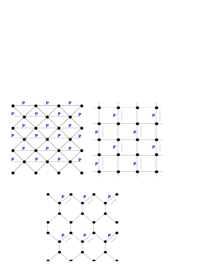
Figure 1: Frustrated Ising spin models: AFM triangle (top left), FF square (top right) and FF honeycomb (bottom). The single bonds represent AFM bonds, the double bonds represent FM bonds, and the perturbed (weakened) bonds in the perturbed Ising models are indicated by “P” (see Section III.2).

II.3 A Generalized Loop Move

Motivated by the above, we introduce a Generalized Loop Move Algorithm (GLM), designed to improve the sampling of equal (or nearly-equal) energy configurations near the groundstates of 2D periodic frustrated Ising models with bond sharing plaquettes. Like previous algorithms designed to work on specific Ising models Barkema and Newman (1998); Melko et al. (2001); Andrews et al. (2009), the algorithm works by identifying groups or clusters of spins that could be flipped together without changing the number of unsatisfied bonds, and then attempting to flip them according to a standard Metropolis update. In this way, no energy costs (proportional to $J$) are accrued, which as mentioned above can inhibit simulation dynamics at low temperatures.

To find these groups of spins, the GLM algorithm uses the concepts of dual graphs and matchings from graph theory. In this paper, dual graphs are defined in the usual graph theory sense. The dual nodes represent the faces/plaquettes in the original (“primal”) spin lattice, and the dual edges connect dual nodes which correspond to faces that share a bond in the primal spin system. See Fig. 2 for how the dual graphs are defined on the triangle, square and honeycomb lattices respectively. If we take a spin system and examine its dual graph, we can consider each dual edge to be inside a pseudo-matching whenever the corresponding bond in the primal spin lattice is unsatisfied. This pseudo-matching is not a matching in the rigorous graph theory sense. In a graph theory matching, each node can only be adjacent to at most one edge in the matching. On the other hand, in the pseudo-matching described in this paper, each dual node can be adjacent to multiple dual edges in the pseudo-matching. There are a few interesting properties to note about this pseudo-matching:

1. In any pseudo-matching that corresponds to a valid spin configuration, each dual node is adjacent to at least one dual edge in the pseudo-matching because each plaquette contains at least one unsatisfied bond in a fully frustrated Ising model.

2. Each plaquette in a fully frustrated Ising model always has an odd number of unsatisfied bonds. Consequently in any pseudo-matching that correspond to a valid spin configuration, each dual node is adjacent to an odd number of dual edges in the pseudo-matching.

3. Each valid ground-state spin configuration and its spin inverse corresponds to a unique pseudo-matching.

4. There is a bijective correspondence between pairs of valid spin configurations and their spin inverses with the minimal number of unsatisfied bonds (one per plaquette) and perfect matchings in the dual graph. A perfect matching is a matching where each node is adjacent to exactly one edge in the matching.

Given a spin configuration, the problem of finding another spin configuration with the same number of unsatisfied bonds is equivalent to finding a pseudo-matching in the dual graph with the same number of dual edges as the pseudo-matching corresponding to the original spin configuration. In graph theory, a basic strategy for finding a new matching, with the same number of edges as an existing matching, is to find an alternating cycle. Given some matching, an alternating cycle consists of edges that are alternatingly inside and outside the matching. For each edge in the alternating cycle, we can add it to the matching if it was not originally in the matching, and remove it from the matching otherwise, to get another matching of with the same number of edges. This operation is known as taking a symmetric difference between the matching and the alternating cycle. The same strategy can be used to find a new pseudo-matching with the same number of dual edges as an existing pseudo-matching. Thus, if we start with a spin configuration and want to find another with the same number of unsatisfied edges, we can consider its corresponding pseudo-matching, use an alternating cycle to find another pseudo-matching, and then map this back to a spin configuration. If we look at this series of actions from the perspective of the spin system, we have found a group of spins delineated by the alternating cycle in the dual graph that can be flipped without changing the number of unsatisfied bonds.

The motivation for looking at the dual graph of the spin system comes from the work by Bieche et. al. Bieche et al. (1980). In that work, the authors devised an algorithm that uses a modified dual graph of a spin system to find its groundstates. The algorithm takes the dual graph of the spin system and modifies it so that there is a bijective correspondence between perfect matchings in the modified dual graph and valid spin configurations. Weights are applied to each edge in the modified dual graph so that the weight of a perfect matching is equal to the energy of the corresponding spin configuration. Consequently, the problem of finding a groundstate in the spin system is transformed into the problem of finding a minimally weighted perfect matching in the dual graph, for which a polynomial time algorithm has been devised by Edmonds et. al. Edmonds (1965a, b). One anticipates that the GLM update, designed in this paper to operate on fully frustrated Ising models, could be extended to work on a broader class of frustrated Ising models by adapting it to use the modified dual graph described in Bieche’s paper.

II.4 Description of the Algorithm

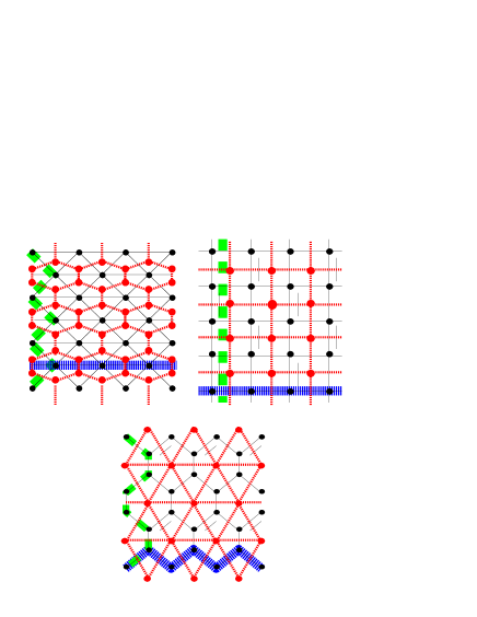
Figure 2: Ising spin models and the corresponding dual graphs: AFM triangle (top left), FF square (top right), and FF honeycomb (bottom). The solid black lines represent primal spin lattice and the thick dashed red lines represent the dual lattice. The dashed shading of primal lattice along the vertical axis represent the Vertical Reference Cut and the hashed shading of primal lattice along the horizontal axis represent the Horizontal Reference Cut.

Like previous loop and cluster algorithms, The Generalized Loop Move (GLM) is designed to supplement single spin flip (SSF) updates. Each iteration of the whole algorithm involves first attempting single spin flips on each spin in the lattice, and then attempting a fixed number of GLMs on the whole lattice. In this paper, we have chosen to perform $N/30$ GLM attempts after each SSF sweep (where $N$ is the number of spins in the lattice). In each GLM attempt, we try to identify a group of spins that can be flipped together without changing the number of unsatisfied bonds in the lattice, compute the probability with which we should accept the flip so as to maintain detailed balance, and then accept the flip according to this probability.

For ease of description, we divide the GLM algorithm into 3 subtasks: the Partition Finding subtask, the Loop Generating subtask and the Acceptance Probability Calculating subtask. The Partition Finding subtask describes how the algorithm finds a group of spins that can be flipped together without changing the number of unsatisfied bonds. The Loop Generating subtask describes how the algorithm finds cycles in the dual graph that are used by the Partition Finding subtask to identify the above-mentioned group of spins. Lastly, the Acceptance Probability Calculating subtask, as the name implies, describes how the algorithm calculates the acceptance probability with which we should accept suggested flips to maintain detailed balance.

To describe the algorithm precisely, we will first establish the following definitions and notations:

1. A bond between spin $i$ and spin $j$ is referred to as $B_{ij}$ and its value is denoted as $J_{ij}\delta_{ij}$ where $J_{ij}$ and $\delta_{ij}$ are defined as in Eq. (1); its dual is referred to as $\widehat{B_{ij}}$.

2. A set of dual edges is called a partition boundary if deleting all the bonds dual to these dual edges would divide the original lattice into two connected components.

3. A Horizontal Reference Cut refers to a specific set of bonds that wraps horizontally around the lattice; a Vertical Reference Cut similarly refers to a specific set of bonds that wraps vertically around the lattice. These reference cuts are used in the algorithm to determine whether a set of dual edges constitutes a partition boundary. The set of bonds chosen is arbitrary. See Fig. 2 for how the Horizontal and Vertical Reference Cuts are defined in this paper on the AFM triangle, FF square and FF honeycomb lattices respectively. Other choices of horizontal and vertical reference cuts that wrap horizontally or vertically around the lattice would work just as well.

4. A cycle is called a simple cycle if it does not intersect itself. If a simple cycle of dual edges in the dual lattice is dual to an even number of bonds in the Horizontal Reference Cut and an even number of bonds in the Vertical Reference Cut, then we refer to the cycle of dual edges as a closed loop. See Fig. 3 for an example of a closed loop. It can be shown that such a cycle of dual edges forms a partition boundary.

5. If a simple cycle of dual edges in the dual lattice is dual to an odd number of bonds in the Horizontal Reference Cut or an odd number of bonds in the Vertical Reference Cut, then we refer to the cycle of dual edges as a cut. See Fig. 3 for an example of a cut. It can be shown that such a cycle of dual edges does not form a partition boundary.

6. If the union of two non-intersecting cuts is dual to an even number of bonds in the Horizontal Reference Cut and an even number of bonds in the Vertical Reference Cut, then it is called a complementary union of cuts. See Fig. 3 for an example of a complementary union of cuts. It can be shown that such a union forms a partition boundary.

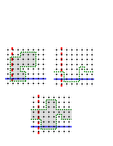
Figure 3: Types of cycles in the dual graph: closed loop (top left), cut (top right), complementary union of cuts (bottom). The dashed shading on the primal lattice along the vertical axis represents the Vertical Reference Cut and the hashed shading of primal lattice along the horizontal axis represents the Horizontal Reference Cut. The dashed green line on the dual graph represents the set of dual edges making up the cycle. The hash shaded area represents the spins enclosed by the Closed Loop or Complementary Union of Cuts.

II.5 Partition Finding Subtask

In the Partition Finding subtask, we try to find a partition boundary that is either a closed loop or a complementary union of cuts. Once we find such a partition boundary, we can use the Acceptance Probability Calculating subtask (Section II.7) to compute the probability with which we should flip all the spins in the smaller of the two partitions formed by the partition boundary so as to maintain detailed balance. Then we flip all the spins inside the smaller of the two partitions with the probability just computed. When all the spins in either partition are flipped, all the satisfied bonds dual to the partition boundary become unsatisfied, all the unsatisfied bonds dual to the partition boundary become satisfied and all other bonds remain unchanged. To ensure that the number of unsatisfied bonds remains unchanged when we flip all the spins inside the partition we want to choose a partition boundary that is dual to an equal number of satisfied and unsatisfied bonds. One way to satisfy this requirement is to choose a partition boundary that is alternatingly dual to satisfied and unsatisfied bonds. To find such a partition boundary, we use the Loop Generating subtask (Section II.6) to find a simple cycle in the dual lattice that is alternating dual to satisfied and unsatisfied bonds. This simple cycle may be a closed loop or a cut. If it is a closed loop, it forms a partition boundary and we have found the desired partition. If it is a cut, then we use the Loop Generating subtask to find a second cycle in the dual lattice. If the second cycle is another cut that does not intersect the first one and the union of the two cycles form a complementary union of cuts, then the union of two cuts forms a partition boundary and we have found the desired partition. If the second cycle does not meet the above requirements, then we abort the Generalized Loop Move. The reason why we want to find complementary unions of cuts is that in perturbed models at $T\ll J$, numerical results have shown that GLM using closed loops alone has a high probability of becoming frozen in a near-groundstate. On the other hand, GLM using a combination of closed loops and union of cuts can efficiently sample from the near-groundstates. It should be noted that when the algorithm finds a cut and then a closed loop, it is possible to discard the cut and keep the closed loop as a partition boundary.

II.6 Loop Generating Subtask

The Loop Generating subtask is designed to find simple cycles of dual edges that are alternatingly dual to satisfied and unsatisfied bonds for the Partition Finding subtask to use. The main idea is that we start at a random dual node in the dual lattice, choose in a random but weighted way one of the dual edges adjacent to the dual node, go to the other dual node adjacent to the dual edge, choose in a random but weighted way a dual edge adjacent to this dual node (we will choose among dual edges dual to satisfied bonds if the last dual edge is dual to an unsatisfied bond and vice versa) and continue this way until we revisit one of the dual nodes we have passed through earlier (i.e. until the string of dual edges ends in a simple cycle). This simple cycle is used by the Partition Finding subtask as described in Section II.5. More precisely, the algorithm can be described as follows:

1. Randomly choose a dual node. Call it $dualnode1$ and the set of dual edges adjacent to it $\widehat{E}$.

2. Randomly select one of the dual edges $\widehat{B_{ij}}$ in $\widehat{E}$. The selection should be completely random for unperturbed models or based on some weighting scheme that favors strong unsatisfied bonds and weak satisfied bonds for perturbed models. When the spins inside the partition are flipped, the bonds dual to the partition boundary are made satisfied if they were previously unsatisfied and unsatisfied if they were previously satisfied. So favoring strong unsatisfied bonds and weak satisfied bonds for inclusion in the cycle means favoring partitions that would decrease the energy of the system if flipped. This increases the likelihood of finding a partition that is energetically favored to be flipped at low temperatures. Numerical results show that a weighting scheme is particularly important for perturbed triangle and square lattices where a GLM algorithm which selects partition boundaries completely at random tends to fail to find partitions that are energetically favored to be flipped in a reasonable amount of time. The weighting scheme chosen by the authors of this paper is:

   $$W(\widehat{B_{ij}})=\begin{cases}e^{\alpha\beta[|J_{ij}|-mean_{\widehat{B_{ij}}\in\widehat{E}}(\{|J_{ij}|\})]}&\text{if $B_{ij}$ is unsatisfied},\\ e^{-\alpha\beta[|J_{ij}|-mean_{\widehat{B_{ij}}\in\widehat{E}}(\{|J_{ij}|\})]}&\text{if $B_{ij}$ is satisfied,}\end{cases}$$ (4)

   where $\beta={1}/{T}$ and $\alpha$ is an arbitrary parameter that affects how strongly the weighting scheme favors weak satisfied bonds and strong unsatisfied bonds . The authors chose $\alpha$ to be 5. Preliminary numerical results showed that an $\alpha$ of 1 did not sufficiently favor partitions that were energetically favored to be flipped. As a result, GLM with an $\alpha$ of 1 showed slow equilibration of thermodynamic data near the groundstate. Consequently, an $\alpha$ of 5 was tried and the thermodynamic data showed fast equilibration.

3. Add this dual edge to our chain of dual edges, go to the other dual node adjacent to this dual edge and repeat the following steps until we revisit a dual node we have already visited:

   1. Call the set of dual edges adjacent to the current dual node $\widehat{E}$

   2. Remove from $\widehat{E}$ all satisfied dual edges if the last dual edge added to our chain is satisfied; otherwise, remove all unsatisfied dual edges.

   3. Remove from $\widehat{E}$ all dual edges that would result in a simple cycle with an odd number of dual edges if selected .

   4. If $\widehat{E}$ is empty, then abort the Generalized Loop Move algorithm and leave the spin configuration unchanged.

   5. Randomly select a dual edge from $\widehat{E}$ based on a weighting scheme that favors dual edges dual to strong unsatisfied bonds or weak satisfied bonds. The author of this paper chose to use the weighting scheme defined by Eq. (4).

   6. Add the dual edge to the chain and go to the dual node on the other end of the dual edge.

4. Once we revisit a node, the simple cycle at the end of our chain of dual edges is the desired simple cycle that we will use in the Partition Finding subtask.

The computation time required to find a simple cycle through the algorithm described above is an important factor in the efficiency of the GLM algorithm. Numerical results concerning the amount of computation time required are discussed in Section III.

II.7 Acceptance Probability Calculating Subtask

Once the Partition Finding subtask generates a partition boundary in the dual graph, the Acceptance Probability Calculating subtask computes an acceptance probability with which the GLM algorithm should flip all the spins inside the smaller partition so as to maintain detailed balance. For ease of exposition, it is convenient to establish the following definitions and notations:

• Define a function $f$ on the set of dual edge chains that end in a simple cycle as follows: If $C=[e_{1\>}e_{2\>}...\>e_{\alpha}\>e_{\alpha+1}\>...\;e_{n-1}\>e_{n}]$ is a chain of dual edges that ends in a simple cycle $L=[e_{\alpha}\>e_{\alpha+1}\>...\;e_{n-1}\>e_{n}]$, then $f(C)=[e_{1\>}e_{2\>}...\>e_{n}\>e_{n-1}\;...\;e_{\alpha+1}\>e_{\alpha}]$. Essentially, $f$ takes a chain of dual edges that end in a simple cycle and reverses the order of dual edges that are part of the simple cycle (see Fig. 4). Note: $f(f(C))=C$.

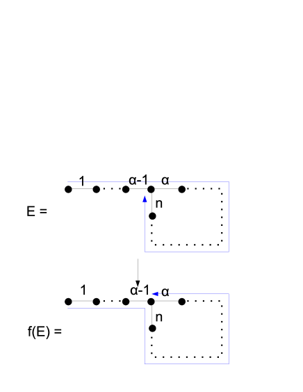
Figure 4: The function $f$ described in the text.

• Let $P_{select}(C,\>S)$ be the probability of the Loop Generating subtask selecting the dual edge chain $C$ under the spin configuration $S$.

• Denote the current spin configuration as $S_{1}$ and the spin configuration after flipping all the spins inside the smaller partition as $S_{2}$.

Then the acceptance probability is defined by the following expressions:

• If the Partition Finding subtask found a partition boundary that is a closed loop $L$ from a chain $C$, then:

  $$P_{accept}(C,\>S_{1})=min\left({1,\>e^{-\beta[E(S_{2})-E(S_{1})]}\frac{P_{select}(f(C),\>S_{2})}{P_{select}(C,\>S_{1})}}\right)$$ (5)

  In the unperturbed case where $E(S_{1})=E(S_{2})$, the expression simplifies to:

  $$P_{accept}(C,\>S_{1})=min\left({1,\>\frac{P_{select}(f(C),\>S_{2})}{P_{select}(C,\>S_{1})}}\right)$$ (6)

• If the Partition Finding subtask found a partition boundary that is a complementary union of cuts $L_{1}\cup L_{2}$ from chains $C_{1}$and $C_{2}$, then:

  $$P_{accept}((C_{1},C_{2}),\>S_{1})=min\left({1,\>e^{-\beta[E(S_{2})-E(S_{1})]}\frac{P_{select}(f(C_{1}),\>S_{2})P_{select}(f(C_{2}),\>S_{2})}{P_{select}(C_{1},\>S_{1})P_{select}(C_{2},\>S_{1})}}\right)$$ (7)

  In the unperturbed case where $E(S_{1})=E(S_{2})$, the expression simplifies to:

  $$P_{accept}((E_{1},E_{2}),\>S_{1})=min\left({1,\>\frac{P_{select}(f(C_{1}),\>S_{2})P_{select}(f(C_{2}),\>S_{2})}{P_{select}(C_{1},\>S_{1})P_{select}(C_{2},\>S_{1})}}\right)$$ (8)

The authors of this paper have chosen to compute $P_{select}(C,S_{1})$ and $P_{select}(f(C),S_{2})$ after a suitable partition boundary has been found.

A rigorous proof of detailed balance is included in Appendix A.

III Simulation results

In this section we examine some prototypical data from Monte Carlo simulations of three frustrated Ising models, using simulations with SSF and GLM updates. In section III.1, thermodynamic data for unperturbed Ising models is compared between simulations employing only SSF, and simulations using both SSF and GLM updates. Some GLM loop properties are characterized. In section III.2, we examine the performance of the GLM updates on the three perturbed Ising models, which are constructed to have a finite-$T$ phase transition to a ground state with a unique spin configuration. We demonstrate that GLM updates helps the simulation find the correct groundstate in cases where SSF updates fail.

III.1 Results on unperturbed models

Metropolis Monte Carlo simulations are performed on the three aforementioned Ising models: AFM triangular, FF square and FF honeycomb (Fig. 1). A typical run employs an annealing technique where the simulation is begun at a high temperature ($T$ = 0.5), and $T$ is gradually lowered through small steps until the system settled in its disordered degenerate groundstate. At each temperature, a fixed number of iterations of either SSF or a combination of SSF and GLM is applied and measurement estimators such as energy and magnetization are collected. Each annealing simulation is performed twice: once with SSF only, and once with a combination of SSF and GLM updates.

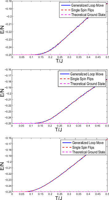
Figure 5: Energy per spin (E/N) for the AFM triangular lattice (top), FF square lattice (middle), and FF honeycomb lattice (bottom). The theoretical true groundstate energy per spin for each system is -0.25

The first numerical result we consider is the internal energy of the Ising models under an annealing simulation. As illustrated in Fig. 5, the internal energy measured as a function of temperature appears identical between SSF and GLM simulations, to within statistical error. This lends practical proof to the fact that the GLM updates are well behaved (do not disrupt detailed balance in the Monte Carlo procedure), and find the same degenerate manifold of states as the SSF updates alone. In addition to annealing simulations, we also tested the performance of SSF and GLM in quenched simulations where the entire simulation (including the warm-up or equilibriation) is run at a single temperature. We ran these single simulations at $T=0.05$, finding that for the case of the AFM triangular and FF square lattice Ising models, both SSF and GLM were able to find a groundstate configuration, the efficiency gain through GLM not being significant in this case. However, for the FF honeycomb lattice, SSF simulations tend to be noticeably slow in finding the disordered groundstate, a situation remedied by employing GLM updates. This difficulty for SSF alone to simulate the low-temperature thermodynamic behavior of the FF honeycomb lattice was also noted in the work by Andrews et. al. Andrews et al. (2009) where a cluster update specific to the FF honeycomb was proposed. In Andrew’s work, it was shown that in an annealing simulation, SSF alone tends to become frozen in one of the groundstates at low temperatures which is evident by the inability of the average magnetization to converge to zero (Fig. 3(c) of Ref. Andrews et al. (2009)). On the other hand, both the algorithm proposed in that paper and GLM can find the correct average magnetization through annealing or quenched simulations.

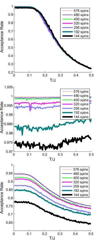
Figure 6: Acceptance Rate of GLM on the AFM triangular lattice (top), FF square lattice (middle), and FF honeycomb lattice (bottom).

A meaningful characterization of the low-temperature dynamics of the GLM updates can be determined via the study of the acceptance rate of the algorithm. We define the acceptance rate as the percentage of GLM attempts that result in successful group spin flips. The results are shown in Fig. 6. For the AFM triangular lattice, the acceptance rate increases as temperature decreases and appears independent of lattice size. For the FF square lattice, the acceptance rate is high across the whole temperature range and appears to approach 1 as lattice size increases. For the FF honeycomb lattice, the acceptance rate is high across the temperature range, increasing as the temperature decreases, and apparently increasing with lattice size. Most importantly, the fact that the acceptance rate is large (of order unity) in all cases, particularly for $T/J\leq 0.1$, suggests that the GLM updates are successful in exploring the manifold of degenerate configurations that contribute to the disordered groundstate. This is in direct contrast to an algorithm employing SSF updates only, which are known to have exponentially suppressed acceptance rates for $T\ll J$.

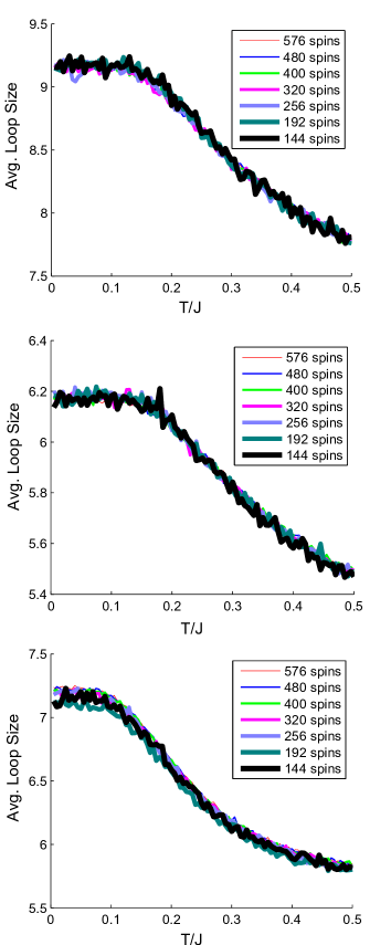
Figure 7: Loop Size for the AFM triangular lattice (top), FF square lattice (middle), and FF honeycomb lattice (bottom).

The average number of dual edges that the GLM algorithm encounters in each successful attempt of the GLM (which we will call chain size), and the average number of dual edges that form the partition boundary (which we will call loop size), provide a measure of the amount of work that the GLM algorithm needs to perform in each iteration. How these two values change with temperature and system size is of interest in determining the efficiency of the algorithm. As illustrated in Fig. 7, for unperturbed FF Ising models, the loop size is independent of lattice size, and increases slightly as temperature decreases. As illustrated in Fig. 8, for unperturbed FF Ising models, the chain size also appears to increase as temperature decreases. Chain size tends to increase with lattice size, however the rate of increase decreases with lattice size, so that the chain size appears to approach a limit as lattice size increases. The increase in chain size with lattice size for smaller systems is likely due to a finite-size effect, meaning that for large lattices both chain size and loop size will saturate. Therefore, the work performed in each GLM attempt is proportional to a fixed multiple of the work performed in each SSF on a single spin. This computational complexity of the GLM attempt is the motivation behind each GLM iteration consisting of one SSF sweep followed by a $N/30$ GLM attempts in this paper. In this way, the work performed in each GLM iteration is expected to be comparable to a fixed multiple of the work performed in a SSF sweep. More rigorous study is required to determine whether the computational complexity of each GLM iteration is a multiple of the work performed in a SSF sweep.

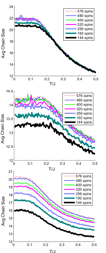
Figure 8: Chain Size for the AFM triangular lattice (top), FF square lattice (middle), and FF honeycomb lattice (bottom).

III.2 Results on perturbed models

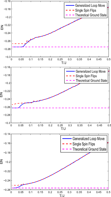
Figure 9: Energy per Spin for the Perturbed AFM triangular lattice (top), Perturbed FF square lattice (middle), and Perturbed FF honeycomb lattice (bottom).

We now explore the effect of anisotropy in the Ising interaction on the performance of the MC algorithm, with SSF and GLM updates. In the following, we define perturbed Ising models by weakening one bond per plaquette in Eq. (1), where two different strengths of $J_{ij}$ are used: $J$ and $J^{\prime}$. The location of weakened bonds are defined via the geometry illustrated in Fig. 1). The one weakened bond per plaquette has the strength $J^{\prime}/J=0.9$. In the AFM triangular case, $\delta_{ij}=1$ for all bonds, and weakened bonds are chosen arbitrarily to occur along the rows of the lattice; in the two FF models, the weakened bond is chosen to correspond to the FM bond with $\delta_{ij}=-1$ for simplicity. In each case, the degenerate manifold of groundstates is lifted resulting in two unique groundstates (related by spin inversion symmetry) where the unsatisfied bonds are placed uniquely at the perturbed bonds. This perturbation presents a greater difficulty for SSF MC algorithms to find the true groundstate. As illustrated in Fig. 9, SSF updates are unable to find the true groundstate energy in any of the three perturbed Ising models through an annealing procedure. GLM updates on the other hand are able to find the true groundstate through annealing (as well as in quenched simulations ran at a single $T\ll J$). It is interesting to note that at low temperatures, the internal energy curve for GLM is noticeably smoother than the internal energy curve for SSF alone. This suggests that GLM is able to converge to the equilibrium faster than SSF alone.

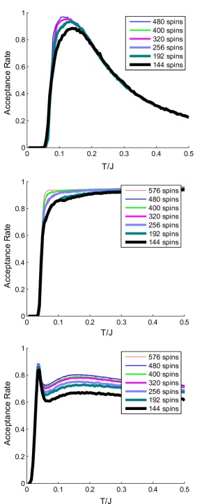
Figure 10: Acceptance Rate of GLM on the Perturbed AFM triangular lattice (top), Perturbed FF square lattice (middle), and Perturbed FF honeycomb lattice (bottom).

As can be seen in Figure 10, for the perturbed AFM triangular lattice model, the acceptance rate of GLM updates increases as the temperature decreases between $T=0.5$ and 0.1, and then sharply drops off to 0 below $T=0.1$. For the perturbed fully frustrated square and honeycomb lattices, the acceptance rate is moderately high and stable between $T=0.5$ and $T=0.05$ and sharply drops to 0 below $T=0.05$. This abrupt drop to zero corresponds to the finite-$T$ phase transition expected to occur in these models at a temperature proportional to the perturbed energy scale, which the GLM updates are able to find cleanly.

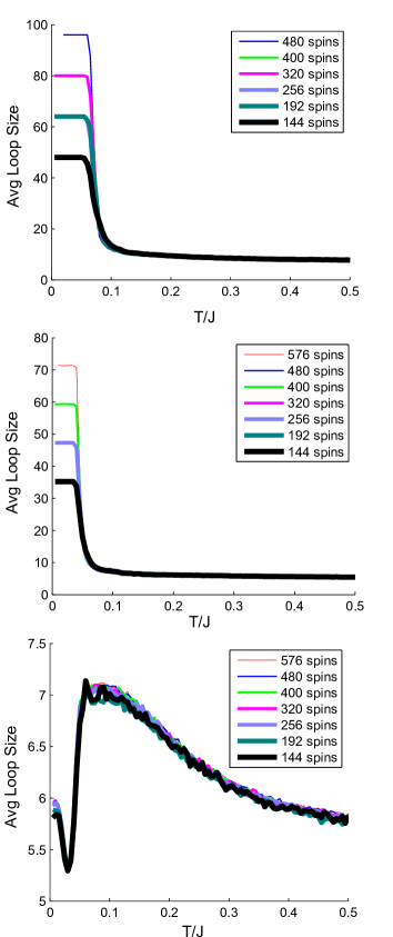
Figure 11: Loop Size for the Perturbed AFM triangular lattice (top), Perturbed FF square lattice (middle), and Perturbed FF honeycomb lattice (bottom).

In the case of perturbed Ising models, temperature has a significant effect on loop and chain size. As illustrated in Figure 11, for perturbed AFM triangle and FF Square lattices, at high temperatures ($T=0.5$ to 0.1) loop size appears independent of lattices size except at low temperatures (below the phase transition) where loop size appears to grow linearly with the shortest side of the lattice. This is expected based on observing GLM updates in action. For perturbed AFM triangle and FF square lattices at low temperatures, the GLM algorithm tends to encounter spin configurations where the only possible partition boundaries are those that wrap around the lattice. For the perturbed FF honeycomb lattice, loop size appears independent of lattice size regardless of temperature. This is also expected because, based on observation, the GLM algorithm tends to find local partition boundaries that do not grow with lattice size at all temperatures. As illustrated in Figure 12, chain size behaves similar to loop size with respect to lattice size and temperature. These results on loop size and chain size suggest that in the groundstate of some perturbed Ising models (such as AFM triangle and FF square) the amount of work the GLM algorithm needs to perform in each GLM attempt will grow linearly with size of the lattice at low temperatures. This suggests that the amount of work done in each GLM iteration (one SSF iteration followed by $x$ attempts of the GLM where $x=N/30$) will grow quadratically with system size at low temperatures. This expensive algorithm cost can be avoided in practical situations by recognizing it as a sign of the underlying long-range order of the system - extensive sampling by the GLM update is not necessary in such a case. Regardless, further simulation results are required to determine the computational complexity of the GLM update in this interesting case.

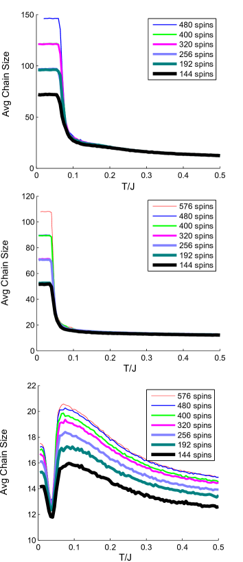
Figure 12: Chain Size for the Perturbed AFM triangular lattice (top), Perturbed FF square lattice (middle), and Perturbed FF honeycomb lattice (bottom).

IV Discussion

In this paper, we have presented a generalized loop move (GLM) update for a class of frustrated Ising models on two-dimensional lattices which are composed of bond-sharing plaquettes. The algorithm is designed to allow efficient Metropolis Monte Carlo updates in a degenerate or quasi-degenerate set of spin configurations that contribute to an extensive manifold of disordered low-energy states. We have thoroughly described the algorithm with the goal of making it easy to implement in a wide variety of models, and have provided a rigorous proof of detailed balance in the general case.

We implemented and tested the algorithm on three prototypical lattice models, the antiferromagnetic triangular-lattice Ising model, and the fully-frustrated square- and honeycomb-lattice Ising models. All three models admit a disordered, extensively-degenerate manifold of configurations in their unperturbed groundstate. The GLM update is demonstrated to complement traditional single spin-flip updates in allowing the simulation to find all configurations that contribute to the degenerate manifold at low temperatures. In contrast to single spin-flips, the GLM update is able to sample configurations in the degenerate subspace with a very high acceptance rate, which is independent of temperature for $T\ll J$. The GLM achieves this while maintaining a very efficient $\mathcal{O}(N)$ complexity for each $N$-site lattice.

Perturbing the models by weakening one bond per plaquette (triangle, square or hexagon) causes them to select a unique spin configuration in their groundstate. Although single spin-flip updates typically cannot find this unique state due to the large energy barriers associated with sampling the quasi-degenerate manifold of states, we have shown that the GLM updates are capable of finding the equilibrium groundstate in a highly efficient manner.

We expect that our current work in describing and characterizing the GLM updates will lead to their use in other frustrated Ising spin models of physical importance. The GLM update, as described in this paper, can be straight-forwardly generalized to work on other frustrated Ising models on two-dimensional lattices of bond-sharing plaquettes. This includes models where the exchange $J_{ij}$ is randomly frustrated, such as Edwards-Anderson spin glass models Bieche et al. (1980), which may facilitate the exploration of spin glass phases and phase transitions in a plethora of related models in the future. Finally, we expect that the GLM moves will be particularly useful in more realistic models of frustrated materials, where additional long-range interactions, local perturbations, or pressure-induced interaction anisotropy leads to the selection of a unique groundstate.

V Acknowledgments

We thank S. Inglis and Geoff Sanders for many useful discussions. This work was made possible by the facilities of the Shared Hierarchical Academic Research Computing Network (SHARCNET:www.sharcnet.ca) and Compute/Calcul Canada. Support was provided by NSERC of Canada.

Appendix A Proof of Detailed Balance

To prove detailed balance, we need to show that given any two spin configurations $S_{1}$ and $S_{2}$, the following equation is satisfied:

$$\Pi(S_{1})T(S_{1}\rightarrow S_{2})=\Pi(S_{2})T(S_{2}\rightarrow S_{1})$$ (9)

where $\Pi(S)$ denotes the Boltzmann probability of spin configuration $S$, and $T(S_{i}\rightarrow S_{j})$ denote the transition probability in the Generalized Loop Move algorithm from spin configuration $S_{i}$ to spin configuration $S_{j}$.

A.1 Preliminary notations and definitions:

For ease of exposition, it is convenient to establish the following notations and definitions:

• Let $\Gamma$ be the set of all possible dual edge chains that the Loop Generating subroutine can generate (i.e. $\Gamma$ is the set of dual edge chains that are alternatingly dual to satisfied and unsatisfied bonds and end in a simple cycle).

• Take any 2 spin configurations $S_{1}$ and $S_{2}$, and let:

  • $\Gamma_{1}=\{\gamma\in\Gamma|\>\gamma$ ends in a closed loop and flipping all the spins inside the closed loop takes the spin system from $S_{1}$ to $S_{2}\}$

  • $\Omega_{1}=\{$$(\gamma_{1},\gamma_{2})\in(\Gamma\times\Gamma)|$$\gamma_{1},\gamma_{2}$ ends in cuts $L_{1},\>L_{2}$ and flipping all the spins inside $L_{1}\cup L_{2}$ takes the spin system from $S_{1}$ to $S_{2}$}

  • $\Psi_{1}=\Gamma_{1}\cup\Omega_{1}$

  • $\Gamma_{2}=\{\gamma\in\Gamma|\>\gamma$ end in a closed loop and flipping all the spins inside the closed loop takes the spin system from $S_{2}$ to $S_{1}\}$

  • $\Omega_{2}=\{$$(\gamma_{1},\gamma_{2})\in(\Gamma\times\Gamma)|$$\gamma_{1},\gamma_{2}$ ends in cuts $L_{1},\>L_{2}$ and flipping all the spins inside $L_{1}\cup L_{2}$ takes the spin system from $S_{2}$ to $S_{1}$}

  • $\Psi_{2}=\Gamma_{2}\cup\Omega_{2}$

  • $\Psi_{1}^{{}^{\prime}}=\{\psi\in\Psi_{1}|\>P_{accept}(\psi,\>S_{1})>0\}$ where $P_{accept}$ is defined as in Equation 5 or 7

  • $\Psi_{2}^{{}^{\prime}}=\{\psi\in\Psi_{2}|\>P_{accept}(\psi,\>S_{2})>0\}$ where $P_{accept}$ is defined as in Equation 5 or 7

  • $\Psi_{1}^{{}^{\prime}}$ and $\Psi_{2}^{{}^{\prime}}$ are defined as above to facilitate the proof of detailed balance.

  • define $F$: $\Gamma\cup(\Gamma\times\Gamma)\rightarrow\Gamma\cup(\Gamma\times\Gamma)$ such that $F(\gamma)=f(\gamma)\;\forall\gamma\in\Gamma$ and $F((\gamma_{1},\gamma_{2}))=(f(\gamma_{1}),\>f(\gamma_{2}))\;\forall(\gamma_{1},\gamma_{2})\in(\Gamma\times\Gamma)$

  • Let $\tilde{F}$ be the restriction of $F$ to $\Psi_{1}^{{}^{\prime}}$

  For convenience, we will also define $P_{select}((\gamma_{1},\gamma_{2}),\>S)=P_{select}(\gamma_{1},\>S)P_{select}(\gamma_{2},\>S)\;\forall(\gamma_{1},\gamma_{2})\in(\Gamma\times\Gamma)$

  Note: $T(S_{i}\rightarrow S_{j})=\sum_{\psi\in\Psi_{i}^{{}^{\prime}}}P_{select}(\psi,\>S_{i})P_{accept}(\psi,\>S_{i})$, where $(i,\>j)=(1,\>2)$ or $(2,\>1)$

A.2 Proof of Detailed Balance

If we can prove the following 3 subclaims:

1. $\tilde{F}(\Psi_{1}^{{}^{\prime}})\subseteq\Psi_{2}^{{}^{\prime}}$ (this is used to prove subclaim 2).

2. $\tilde{F}$ is bijective between $\Psi_{1}^{{}^{\prime}}$ and $\Psi_{2}^{{}^{\prime}}$.

3. $\forall\psi\in\Psi^{{}^{\prime}}_{1},$ $\Pi(S_{1})P_{select}(\psi,\>S_{1})P_{accept}(\psi,\>S_{1})=\Pi(S_{2})P_{select}(\tilde{F}(\psi),\>S_{2})P_{accept}(\tilde{F}(\psi),\>S_{2})$.

Then, the proof for detailed balance follows naturally:

$${\displaystyle\Sigma_{\psi\in\Psi_{1}^{{}^{\prime}}}\Pi(S_{1})P_{select}(\psi,\>S_{1})P_{accept}(\psi,\>S_{1})=\Sigma_{\psi\in\Psi_{1}^{{}^{\prime}}}\Pi(S_{2})P_{select}(\tilde{F}(\psi),\>S_{2})P_{accept}(\tilde{F}(\psi),\>S_{2})}$$

by subclaim 3

$$\Rightarrow {\displaystyle\Sigma_{\psi\in\Psi_{1}^{{}^{\prime}}}\Pi(S_{1})P_{select}(\psi,\>S_{1})P_{accept}(\psi,\>S_{1})=\Sigma_{\delta\in\Psi_{2}^{{}^{\prime}}}\Pi(S_{2})P_{select}(\delta,\>S_{2})P_{accept}(\delta,\>S_{2})}$$

because $$\tilde{F} \Psi_{1}^{{}^{\prime}} \Psi_{2}^{{}^{\prime}}$$is bijective between and

$$\Rightarrow {\displaystyle\Pi(S_{1})\Sigma_{\psi\in\Psi_{1}^{{}^{\prime}}}P_{select}(\psi,\>S_{1})P_{accept}(\psi,\>S_{1})=\Pi(S_{2})\Sigma_{\delta\in\Psi_{2}^{{}^{\prime}}}P_{select}(\delta,\>S_{2})P_{accept}(\delta,\>S_{2})}$$

$$\Rightarrow \Pi(S_{1})T(S_{1}\rightarrow S_{2})=\Pi(S_{2})T(S_{2}\rightarrow S_{1})$$

A.3 Proof of subclaims

Subclaim 1: $\tilde{F}(\Psi_{1}^{{}^{\prime}})\subseteq\Psi_{2}^{{}^{\prime}}$

Take any $\psi\in\Psi_{1}^{{}^{\prime}}$, show that $\tilde{F}(\psi)\in\Psi_{2}^{{}^{\prime}}$

1. $\tilde{F}(\psi)\in\Psi_{2}$ because:

   1. $\psi\in\Psi_{1}$ implies $\psi$ ends in a closed loop or union of complementary cuts that forms a partition boundary around a group of spins that if flipped will take the spin configuration from $S_{1}$ to $S_{2}$. Therefore, $\tilde{F}(\psi)$ ends in a closed loop or union of complementary cuts that forms a partition boundary around the same group of spins, which if flipped will take the spin configuration from $S_{2}$ back to $S_{1}$

   2. and $P_{select}(\tilde{F}(\psi),\;S_{2})>0$ because

      $$\psi\epsilon\in\Psi_{1}^{{}^{\prime}} \Rightarrow P_{accept}(\psi,\>S_{1})>0$$

      $$\Rightarrow min(1,\;e^{-\beta[E(S_{2})-E(S_{1})]}\frac{P_{select}(\tilde{F}(\psi),\;S_{2})}{P_{select}(\psi,\;S_{1})})>0$$

      $$\Rightarrow P_{select}(\tilde{F}(\psi),\;S_{2})>0$$

2. $$P_{accept}(\tilde{F}(\psi),\;S_{2})=min(1,\;e^{-\beta[E(S_{2})-E(S_{1})]}\frac{P_{select}(\psi,\>S_{1})}{P_{select}(\tilde{F}(\psi),\>S_{2})})>0$$

   because $\psi\in\Psi_{1}^{{}^{\prime}}\subseteq\Psi_{1}\Rightarrow P_{select}(\psi,\>S_{1})>0$.

3. 1 & 2 $\Longrightarrow\tilde{F}(\psi)\in\Psi_{2}^{{}^{\prime}}$. Therefore, $\tilde{F}(\Psi_{1}^{{}^{\prime}})\subseteq\Psi_{2}^{{}^{\prime}}$

Subclaim 2: $\tilde{F}$ is bijective between $\Psi_{1}^{{}^{\prime}}$ and $\Psi_{2}^{{}^{\prime}}$

1. $\tilde{F}$ is injective because $\tilde{F}(\Psi_{1}^{{}^{\prime}})\subseteq\Psi_{2}^{{}^{\prime}}$ by subclaim 1 and take any $\psi_{1}$, $\psi_{2}$ $\in\Psi_{1}$, $\tilde{F}(\psi_{1})=\tilde{F}(\psi_{2})\Rightarrow\psi_{1}=\psi_{2}$ by definition of $f()$

2. $\tilde{F}$ is subjective because for any $\delta\in\Psi_{2}^{{}^{\prime}}$, $F(\delta)\in\Psi_{1}^{{}^{\prime}}$ by subclaim 1, and $\tilde{F}(F(\delta))=\delta$.

Subclaim 3: For any $\psi\in\Psi^{{}^{\prime}}_{1}$, show that $\Pi(S_{1})P_{select}(\psi,\>S_{1})P_{accept}(\psi,\>S_{1})=\Pi(S_{2})P_{select}(\tilde{F}(\psi),\>S_{2})P_{accept}(\tilde{F}(\psi),\>S_{2})$

Let $a=\Pi(S_{1})P_{select}(\psi,\>S_{1})$, and $b=\Pi(S_{2})P_{select}(\tilde{F}(\psi),\>S_{2})$. Then,

$$\Pi(S_{1})P_{select}(\psi,\>S_{1})P_{accept}(\psi,\>S_{1}) = \Pi(S_{1})P_{select}(\psi,\>S_{1})\min(1,\frac{\Pi(S_{2})}{\Pi(S_{1})}\frac{P_{select}(\tilde{F}(\psi),\>S_{2})}{P_{select}(\psi,\>S_{1})})$$

$$= a\>\min(1,\>\frac{b}{a})$$

$$= \min(a,\>b)$$

$$\Pi(S_{2})P_{select}(\tilde{F}(\psi),\>S_{2})P_{accept}(\tilde{F}(\psi),\>S_{2}) = \Pi(S_{2})P_{select}(\tilde{F(}\psi),\>S_{2})\min(1,\frac{\Pi(S_{1})}{\Pi(S_{2})}\frac{P_{select}(\psi,\>S_{1})}{P_{select}(\tilde{F}(\psi),\>S_{2})})$$

$$= b\>\min(1,\>\frac{a}{b})$$

$$= \min(a,\>b)$$

Therefore $\Pi(S_{1})P_{select}(\psi,\>S_{1})P_{accept}(\psi,\>S_{1})=\Pi(S_{2})P_{select}(\tilde{F}(\psi),\>S_{2})P_{accept}(\tilde{F}(\psi),\>S_{2})$

References

- Metropolis et al. (1953) N. Metropolis, A. W. Rosenbluth, M. N. Rosenbluth, A. H. Teller, and E. Teller, J. Chem. Phys. 21, 1087 (1953).
- Liu (2001) J. Liu, Monte Carlo Strategies in Scientific Computing (Springer, 2001).
- Moore (1965) G. E. Moore, Electronics 38, 8 (1965).
- Swendsen and Wang (1987) R. H. Swendsen and J.-S. Wang, Phys. Rev. Lett. 58, 86 (1987).
- Wolff (1989) U. Wolff, Phys. Rev. Lett. 62, 361 (1989).
- Wannier (1950) G. H. Wannier, Phys. Rev. 79, 357 (1950).
- Houtappel (1950) R. M. F. Houtappel, Physica 16, 425 (1950).
- Barkema and Newman (1998) G. T. Barkema and M. E. J. Newman, Phys. Rev. E 57, 1155 (1998).
- Bramwell and Gingras (2001) S. T. Bramwell and M. J. P. Gingras, Science 294, 1495 (2001).
- Melko et al. (2001) R. G. Melko, B. C. den Hertog, and M. J. P. Gingras, Phys. Rev. Lett. 87, 067203 (2001).
- Shinaoka and Motome (2010) H. Shinaoka and Y. Motome (2010), eprint arXiv:1006.4300.
- Orendáč et al. (2007) M. Orendáč, J. Hanko, E. Čižmár, A. Orendáová, M. Shirai, and S. T. Bramwell, Phys. Rev. B 75, 104425 (2007).
- Jaubert et al. (2008) L. D. C. Jaubert, J. T. Chalker, P. C. W. Holdsworth, and R. Moessner, Phys. Rev. Lett. 100, 067207 (2008).
- Jaubert et al. (2010) L. D. Jaubert, J. Chalker, P. C. Holdsworth, and R. Moessner, arXiv:1003.4896 (2010).
- Andrews et al. (2009) S. Andrews, H. De Sterck, S. Inglis, and R. G. Melko, Phys. Rev. E 79, 041127 (2009).
- Moessner and Sondhi (2001) R. Moessner and S. L. Sondhi, Phys. Rev. B 63, 224401 (2001).
- Fisher (1961) M. E. Fisher, Phys. Rev. 124, 1664 (1961).
- Wolff and Zittartz (1982) W. F. Wolff and J. Zittartz, Z. Phys. B 49, 129 (1982).
- Bieche et al. (1980) I. Bieche, R. Maynard, R. Rammal, and J. P. Uhry, Journal of Physics A 13, 2553 (1980).
- Edmonds (1965a) J. Edmonds, Can. J. Math. 17, 449 (1965a).
- Edmonds (1965b) J. Edmonds, J. Res. NBS. 69B, 125 (1965b).