Galactic foregrounds: Spatial fluctuations and a procedure of removal

Abstract

Present day cosmic microwave background (CMB) studies require more accurate removal of Galactic foreground emission. This removal becomes even more essential for CMB polarization measurements. In this paper, we consider a way of filtering out the diffuse Galactic fluctuations on the basis of their statistical properties, namely, the power-law spectra of fluctuations. We focus on the statistical properties of two major Galactic foregrounds that arise from magnetized turbulence, namely, diffuse synchrotron emission and thermal emission from dust and describe how their power laws change with the Galactic latitude. We attribute this change to the change of the geometry of the emission region and claim that the universality of the turbulence spectrum provides a new way of removing Galactic foregrounds. For the Galactic synchrotron emission, we mainly focus on the geometry of the synchrotron emitting regions, which will provide useful information for future polarized synchrotron emission studies. Our model calculation suggests that either a one-component extended halo model or a two-component model, an extended halo component (scale height $\gtrsim 1kpc$) plus a local component, can explain the observed angular spectrum of the synchrotron emission. For thermal emission from Galactic dust, we discuss general properties of a publicly available 94GHz total dust emission map and explain how we can obtain a polarized dust emission map. Based on a simple model calculation, we obtain the angular spectrum of the polarized dust emission. Our model calculation suggests that $C_{l}\propto l^{-11/3}$ for $l\gtrsim 1000$ and a shallower spectrum for $l\lesssim 1000$. We discuss and demonstrate how we can make use of our findings to remove Galactic foregrounds using a template of spatial fluctuations. In particular, we consider examples of spatial filtering of a foreground at small scales, when the separation into CMB signal and foregrounds is done at larger scales. We demonstrate that the new technique of spatial filtering of foregrounds may be promising for recovering the CMB signal in a situation when foregrounds are known at a scale different from the one under study. It can also improve filtering by combining measurements obtained at different scales.

1. Introduction

An important problem in the studies of the early universe with the CMB fluctuations is related to separating them from Galactic foregrounds. The techniques of removing foregrounds are rather elaborate, but in most cases they include using the frequency templates of foreground emission. This requires multi-frequency measurements, which are not always available. Moreover, some foregrounds, e.g. the so-called spinning dust (Draine & Lazarian 1998ab; Finkbeiner et al. 2002; Lazarian & Finkbeiner 2003), demonstrate rather complex frequency dependence. Due to the utmost importance of obtaining CMB signal free of contamination, it is essential to consider other ways to remove foregrounds. One way to do this is to take into account the known spatial properties of emission.

If a foreground has well-defined statistics of spatial fluctuations, one can devise techniques of removing the contribution of the foreground to the measured microwave signal (see §2). The issue in this case is whether foregrounds have well defined behavior in terms of their spatial statistics. Determining this with the available data is the first thrust of our present study which we pursue using the Galactic synchrotron and the Galactic dust emission data. The second thrust is devising possible ways of removing the foregrounds using the self-similarity of Galactic turbulence that gives rise to the foreground fluctuations.

This work continues our brief study in Cho & Lazarian (2002a, henceforth CL02) where we argued that the properties of Galactic foreground radiation can be explained on accepting that the interstellar medium (ISM) that provides the fluctuations is turbulent and therefore the spatial fluctuations of foregrounds inherit power-law spectra of the underlying magnetohydrodynamic (MHD) turbulence. Since that work, better understanding of the properties of the MHD turbulence has been achieved. For instance, it became clear that the spectrum of density in compressible MHD turbulence can be substantially shallower than the Kolmogorov spectrum that we assumed in CL02 (see Beresnyak, Lazarian & Cho 2005). Moreover, the search for alternative procedures of removing foregrounds became more essential with the attempts to measure the polarization of the CMB radiation, especially the enigmatic $B$-modes. The latter motivates choice of foregrounds that we deal with in the present paper. Synchrotron and dust emissions are the sources of the polarized contamination for the CMB polarization studies.

Diffuse Galactic synchrotron emission is an important polarized foreground source, the understanding of which is essential for CMB studies, especially, in the range of 10-100 GHz. It is known that the observed spectra of synchrotron emission and synchrotron polarization (see de Oliveira-Costa & Tegmark 1999 and references therein) reveal a range of power laws. The polarization of synchrotron emission traces magnetic fields and is perpendicular to the plane-of-sky magnetic field direction. Since the Galactic synchrotron emissivity is roughly proportional to the magnetic energy density, angular spectrum of synchrotron emission reflects statistics of magnetic field fluctuations in the Galaxy (see §A.1 for discussions).

Thermal emission from dust is also an important source of polarized foreground emission in the range of frequencies larger than 60 GHz. The emission gets polarized due to grain alignment (see Lazarian 2007 for a review). Therefore, polarization of dust, similar to synchrotron polarization, traces magnetic field fluctuations.

What is the cause of the magnetic field fluctuations? As magnetic field lines are twisted and bend by turbulent motions in the Galaxy it is natural to think of the turbulence as the origin of the magnetic field fluctuations. In fact, several earlier studies addressed the relation between turbulence and the diffuse synchrotron foreground radiation. Tegmark et al. (2000) suggested that the spectra may be relevant to Kolmogorov turbulence. Chepurnov (1999) and CL02 used different approaches, but both showed that the angular spectrum of synchrotron emission reveals Kolmogorov spectrum ($C_{l}\propto l^{-11/3}$) for large values of multipole $l$. However, they noted that the spectrum can be shallower than the Kolmogorov one for smaller values of multipole $l$, due to density stratification in the halo (Chepurnov 1999) or the Galactic disk geometry (CL02).

Recent research of compressible magnetized turbulence suggests that the fluctuations may not be necessarily Kolmogorov, to start with (see Beresnyak et al. 2005; Kowal & Lazarian 2007). Nevertheless, both observations and numerical studies confirm the power-law dependence of turbulence, even if the spectrum differs from the Kolmogorov one. This is also supported by theory, which states the self-similarity of turbulence. It is this self-similarity that gives us hope for a successful removal of foregrounds arising from turbulent interstellar media.

At the same time, it is known that the spatial spectral index of foregrounds measured for different Galactic latitudes may differ. If the reason for this is unknown, this may make the weeding out of foregrounds using spatial templates unreliable. CL02 identified these changes with the variations of the geometry of the emission region. Thus, for the same Galactic latitudes one should expect the same slope of the spatial spectrum of the fluctuations, which, for instance, allows one to extend the power-law spectrum of fluctuations measured for low spherical harmonics to higher spherical harmonics. Potentially, if the geometry of the emission region is known, this allows us to predict the expected changes of the index. In this paper we provide more support for the conjecture in CL02.

In this paper, we first present general properties and structure functions of a publicly available synchrotron foreground emission map. Then we investigate what kinds of Galactic halo structures can produce the observed structure function (and therefore angular spectrum), which will be useful for the study of polarized synchrotron foreground. We also present the properties of a publicly available model dust emission map. Dust emission is one of the most important sources of polarized foreground radiation. Therefore, measurement of angular power spectrum of such foreground is of great interest. Thus, we provide estimation of angular spectrum of polarized emission by foreground dust. This result is of great importance in view of recent interest to the CMB polarization. In §2 we explain a way of spatial removal of foreground emission and provide the summary of the expected scaling of foreground fluctuations arising from Galactic turbulence. In §3, we present statistical analysis of the Haslam map, which is dominated by diffuse Galactic synchrotron emission. In §4, we investigate polarized emission from thermal dust. In §5, we discuss how to utilize our knowledge to remove Galactic foregrounds. We provide the discussion of our results in §6 and the summary in §7. In Appendix, we review a simple model of the angular spectrum of synchrotron emission arising from MHD turbulence. In Appendix, we also present calculations of high-order structure functions of the synchrotron and the dust maps and we compare the results with those of turbulence.

2. Motivation: a new technique of foreground removal

2.1. Spatial Removal of Foregrounds

Let us illustrate a possible procedure of the removal of Galactic foregrounds from the CMB signal. The cosmic microwave signals consists of the CMB signal $I^{CMB}$ and foregrounds $I^{F}$. When we correlate the microwave signal at points “1” and “2”, we get

$$\langle(I^{CMB}_{1}+I^{F}_{1})(I^{CMB}_{2}+I^{F}_{2})\rangle=\langle I^{CMB}_{1}I^{CMB}_{2}\rangle+\langle I^{F}_{1}I^{F}_{2}\rangle,$$ (1)

where we assume $I^{CMB}$ and $I^{F}$ are uncorrelated. Therefore, the measured angular spectrum $C^{measured}_{l}$ is just the sum of $C^{CMB}_{l}$ and $C^{F}_{l}$ and we have

$$C^{CMB}_{l}=C^{measured}_{l}-C^{F}_{l}.$$ (2)

That is, if we know the angular spectrum of foregrounds $C^{F}_{l}$, we can obtain the CMB angular spectrum $C^{CMB}_{l}$.

How can one obtain $C^{F}_{l}$? The well tested way of doing this is to use multi-frequency measurements of the CMB + foreground emission and separate the two components using the frequency templates of foregrounds. This approach requires many measurements at different frequencies. In addition, for some foregrounds the frequency templates may be difficult to obtain. The so-called ”spinning dust” foreground introduced in Draine & Lazarian (1998ab) presents an example of such a difficult-to-remove foreground. We also mention that the measurements of foregrounds at different frequencies may have different spatial resolutions and the use of the maps with different resolutions may also present a problem.

In this paper we address a somewhat different problem, which in its extreme can be formulated in the following way. Imagine that we separated the foreground and the CMB signals at low resolution $l_{low}$ using the traditional multifrequency approach. Is it possible to use this information to remove the foreground contribution from $C^{measured}_{l}$ for $l>l_{low}$? For instance, the measurements of the Wilkinson Microwave Anisotropy Probe (WMAP) provide a high accuracy measure of $C^{F}_{l}$ over a limited range of scales. If we know $C^{F}_{l}$ as a function of $l_{low}$ at scales smaller than those measured by the WMAP, then one can extrapolate $C^{F}_{l}$ to $l>l_{low}$. These values of $C^{F}_{l}$ can be used to filter the microwave measurements from balloon-born experiments using the procedure given by Eq. (2). Note that the balloon-born experiments usually have higher spatial resolutions, but not enough frequency coverage to remove foregrounds using the frequency templates.

The key question is to what extend we can predict $C^{F}_{l}$ over a range of scales which is different from the range of scales at which $C^{F}_{l}$ was measured. The answer to this question is trivial if $C^{F}_{l}$ is a simple power law. While the actual spectra of foregrounds are more complex, in this paper we provide both theoretical arguments and the analysis of the foreground data which support the notion that $C^{F}_{l}$ can be successfully extended beyond the range of $l$ which is measured.

We should stress that the filtering above is different from the accepted techniques of foreground removal using frequency-dependent templates. The outcome of the latter procedures are maps of the foreground radiation and the CMB radiation. The filtering described above is of statistical nature. The result of it is $C^{CMB}_{l}$ rather than emission maps.

In view of above, it is important to determine to what extend the spatial properties of $C^{F}_{l}$ are predictable, in particular, explore to what extend the power-law approximation is applicable. This paper provides a study of spatial statistical properties of fluctuations of synchrotron and dust emission and relates those to the properties of the underlying turbulence. It also provides an example of the filtration procedure that we advocate.

Another important issue is to determine the reasons for the change of the power law behavior with latitude. This is what we study below for the synchrotron and dust foreground emissions. The ultimate goal of this research is to obtain models of Galactic foregrounds which provide a good fit for the foreground spatial spectrum at arbitrary scales and arbitrary latitudes. This paper is a step to constructing such a model.

2.2. Power-law behavior of interstellar turbulence

For the spatial removal procedure to work, we should understand the spatial spectra of foregrounds. Since the spatial fluctuations of foregrounds inherit the spectra of the underlying interstellar turbulence, we summarize the spectral behavior of interstellar turbulence.

It is generally accepted that the interstellar medium (ISM) is magnetized and turbulent (see reviews by Elmegreen & Scalo 2004 and McKee & Ostriker 2007). The so-called ”Big Power Law in the Sky” corresponding to the Kolmogorov-type turbulence was reported in Armstrong, Rickett, & Spangler (1995). Recently this law based on the measurements of the radio scintillations arising from electron density inhomogeneities has been extended to larger scales using the WHAM H_α fluctuations (Chepurnov & Lazarian 2010).

Spectra of magnetic turbulence has been studied using Faraday rotation measurements (see Haverkorn et al. 2008) and starlight polarization (Hildebrand et al. 2009). The interpretation of the results are more challenging in those cases.

Molecular and atomic spectral lines present a very promising way of studying turbulence. The interstellar lines are known to be Doppler-broadened due to turbulent motions. Obtaining spectra from Doppler-broadened lines is not trivial, however. A lot of research in this direction based on the use of the so-called ”velocity centroids”, which were the main tool to study velocity fluctuations, has been shown to produce erroneous results for supersonic turbulence (Lazarian & Esquivel 2003; Esquivel & Lazarian 2005; Esquivel et al. 2007). At the same time new techniques based on the theoretical description of the Position-Position-Velocity (PPV) data cubes, namely, the Velocity Channel Analysis (VCA) and the Velocity Coordinate Spectrum (VCS) have been developed (Lazarian & Pogosyan 2000, 2004, 2006, 2008), tested (see Stanimirovic & Lazarian 2001; Lazarian, Pogosyan, & Esquivel 2002; Esquivel et al. 2003; Chepurnov & Lazarian 2009; Padoan et al. 2006, 2009) and applied to the observational data to obtain the characteristics of the velocity turbulence (see Lazarian 2009 for a review).

VCA and the VCS techniques reveal that the velocities for interstellar turbulence may be somewhat steeper than the Kolmogorov one , while the density spectra of the fluctuations may be substantially more shallow than the spectrum of Kolmogorov fluctuations (see Padoan et al. 2006, 2009; Chepurnov et al. 2010). This agrees well with the numerical studies of the magnetized supersonic turbulence (Beresnyak, Lazarian & Cho 2005; Kowal, Lazarian & Beresnyak 2007; Kowal & Lazarian 2010). For the subsonic turbulence the spectrum of magnetized media gets the values close to the Kolmogorov index (see Goldreich & Sridhar 1995; Lazarian & Vishniac 1999; Cho & Vishniac 2000; Muller & Biskamp 2000; Maron & Goldreich 2001; Lithwick & Goldreich 2001; Cho, Lazarian & Vishniac 2002; Cho & Lazarian 2002b, 2003; Boldyrev 2006; Beresnyak & Lazarian 2006, 2009). In view of that we believe that the Kolmogorov spectrum can be used as a proxy of the underlying spectra of velocity and magnetic field, while a more cautious approach should be demonstrated to density in highly compressible environments, e.g. molecular clouds.

Below we shall show that the spectra of turbulence derived from the analysis of foreground is consistent with both the results of dedicated observations of turbulence as well as the theoretical expectation for the MHD turbulence.

2.3. Data Sets

We use the 408MHz Haslam all-sky map (Haslam et al. 1982) and a model 94GHz dust emission map that are available on the NASA’s LAMBDA website . Both maps were reprocessed for HEALPix (Górski et al. 2005) with nside=512 (7^′ resolution).

The original Haslam data were produced by merging several different data-sets. “The original data were processed in both the Fourier and spatial domains to mitigate baseline striping and strong point sources” (see the website for details). The angular resolution of the original Haslam map is $\sim 1^{\circ}$. Galactic diffuse synchrotron emission is the dominant source of emission at 408MHz.

The 94 GHz dust emission map is based on the work of Schlegel, Finkbeiner, & Davis (1998) and Finkbeiner, Davis, & Schlegel (1999). Schlegel et al. (1998) combined 100$\mu m$ maps of IRAS (Infrared Astronomy Satellite) and DIRBE (Diffuse Infrared Background Experiment on board the COBE satellite) and removed the zodiacal foreground and point sources to construct a full-sky map. Finkbeiner et al. (1999) extrapolated the 100$\mu m$ emission map and 100/240$\mu m$ flux ratio maps to sub-millimeter and microwave wavelengths. The 94 GHz dust map we used is identical to the two-component model 8 of Finkbeiner et al. (1999). The angular resolution of the 100-micron map is $\sim 6^{\prime}$ and that of the temperature correction derived from the 100/240-micron ratio map is $\sim 1^{\circ}$ (Finkbeiner et al. 1999), which corresponds to $l\sim 180^{\circ}/\theta^{\circ}\sim 180$.

3. Spatial statistics of Diffuse Galactic Synchrotron Emission

In this section, we analyze the Haslam 408MHz all-sky map, which is dominated by Galactic diffuse synchrotron emission. Our main goal is to explain the observed synchrotron angular spectrum using simple turbulence models. The result in this section will be useful for sophisticated modeling of polarized synchrotron emission.

3.1. General properties of diffuse Galactic synchrotron emission

In this section, we study synchrotron emission from the Galactic halo (i.e. $b\gtrsim 30^{\circ}$) and the Galactic disk (i.e. $|b|\leq 2^{\circ}$) separately. Our main goal is to see if statistics of synchrotron emission from the halo is consistent with turbulence models. When it comes to synchrotron emission from the Galactic disk, it is not easy to separate diffuse emission and emission from discrete sources. Therefore, we do not try to study turbulence in the Galactic disk. Instead, we will try to estimate which kind of emission is dominant in the Galactic disk.

There exist several models for the diffuse Galactic radio emission. Beuermann, Kanbach, & Berkhuijen (1985) showed that a two-component model, a thin disk embedded in a thick disk, can explain observed synchrotron latitude profile. They claimed that the equivalent width of the thick disk is about several kiloparsecs and thin disk has approximately the same equivalent width as the gas disk. They assumed that, in the direction perpendicular to the Galactic plane, the emissivity $\epsilon$ of each component follows

$$\epsilon(z)=\epsilon(0)sech^{b}(z/z_{0}),$$ (3)

where $z$ is the distance from the Galactic plane and $\epsilon(0)$, $b$, and $z_{0}$ are constants. The half-equivalent width of the disk, which is proportional to $z_{0}$, at the location of the Sun is $\sim 2$kpc.

Recently, several Galactic synchrotron emission models have been proposed in an effort to separate Galactic components from the WMAP polarization data (see, for example, Page et al. 2007; Sun et al. 2008; Miville-Deschenes et al. 2008; Waelkens et al. 2008). All the models mentioned above assume the existence of a thick disk component with a scale height equal to $1~{}kpc$. Sun et al. (2008) considered an additional local spherical component motivated by the local excess of the synchrotron emission that might be related to the “local bubble” (see, for example, Fuchs et al. 2008).

The detailed modeling of the Galactic synchrotron emission is beyond the scope of our paper. We will simply assume that there is a thick component with a scale height of $\sim 1$kpc. We will also assume that there could be an additional local spherical component. Then, in the following subsections, we will consider the relation between spectrum of 3-dimensional turbulence and the observed angular spectrum of synchrotron emission.

Figure 1.— Haslam 408MHz map. Left: Second-order angular structure function (for $b>30^{\circ}$) shows a slope of $\sim 1.2$, which is shallower than that of Kolmogorov turbulence (slope $=5/3$). Right: Structure function as a function of Galactic latitude. From bottom to top, the second-order angular structure functions are obtained for thin stripes ($|\Delta b|\leq 2^{\circ}$) along Galactic latitudes of $30^{\circ}$, $10^{\circ}$, and $0^{\circ}$.

3.2. Structure function of the 408MHz Haslam map

In Appendix, we discussed the relation between the 3D spatial MHD turbulence spectrum and the observed 2D angular spectrum of synchrotron emission (see Eq. [A11] for a quick summary). But, in Appendix we assumed that the emission arises from a spherical region filled with homogeneous turbulence. In this section, we will show that the modulation of synchrotron intensity of the emitting volume can also affect the observed angular spectrum of synchrotron emission.

Earlier studies showed that the angular spectrum 408-MHz Haslam map has a slope close to $-3$: $C_{l}\propto l^{-3}$ (Tegmark & Efstathiou 1996; Bouchet, Gispert, & Puget 1996). Recently La Porta et al. (2008) performed a comprehensive angular power spectrum analysis of all-sky total intensity maps at 408MHz and 1420MHz. They found that the slope is close to -3 for high Galactic latitude regions. Other results also show slopes close to -3. For example, using Rhodes/HartRAO data at 2326 MHz (Jonas, Baart, & Nicolson 1998), Giardino et al. (2001b) obtained a slope $\sim 2.92$ for high Galactic latitude regions with $|b|>20^{\circ}$. Giardino et al. (2001a) obtained a slope $\sim 3.15$ for high Galactic latitude regions with $|b|>20^{\circ}$ from the Reich & Reich (1986) survey at 1420 MHz. Bouchet & Gispert (1999) also obtained a slope $\sim l^{-3}$ spectrum from the 1420 MHz map.

In general, synchrotron emission from the Galactic disk makes it difficult to measure the angular spectrum of synchrotron emission from the Galactic halo. In order to avoid the contamination by the Galactic disk, one may mask out the low Galactic latitude regions. This can be done, for example, by setting all synchrotron intensity to zero for regions with $|b|<b_{cut}$. However, the angular spectrum obtained with the Galactic mask exhibits spurious oscillations. Moreover, the spectrum obtained with a mask may not be the true one because it is contaminated by the mask. In principle, one may correct such oscillations and estimate the true spectrum, using the convolution theorem: the Fourier coefficients (or, in this case, spherical harmonic coefficients) of the masked data are convolution of those of the true data and those of the mask. However, the practical implementation of the method is not simple.

Another approach is to estimate 2-point correlation function first and to extract the angular power spectrum from it (Szapudi et al. 2001; see also Eq. [10]). This method is free of artifacts caused by the mask. But the angular spectrum $C_{l}$ obtained in this way is, in general, noisy and it requires a lot of calculations to accurately measure the slope of the spectrum.

We are interested in the slope of the angular spectrum on small angular scales, which is the same as that of the underlying 3D spatial turbulence spectrum (see Appendix). Therefore, in this paper, we use yet another approach. We first calculate the second-order angular structure function:

$$D_{2}(\theta)=<|I({\bf e}_{1})-I({\bf e}_{2})|^{2}>,$$ (4)

where $I({\bf e})$ is the intensity of synchrotron emission, ${\bf e}_{1}$ and ${\bf e}_{2}$ are unit vectors along the lines of sight, $\theta$ is the angle between ${\bf e}_{1}$ and ${\bf e}_{2}$, and the angle brackets denote average taken over the observed region. Then, we extract the slope of the angular spectrum using the relation

$$D_{2}(\theta)\propto\theta^{m-2}\Leftrightarrow C_{l}\propto l^{-m}\Leftrightarrow E_{3D}\propto k^{-m}$$ (5)

for small angular scales (see §A.2).

We note that excessive care is required in the presence of white noise. In the presence of white noise, second-order structure function will be $D_{2}(\theta)=<|I({\bf e}_{1})+\delta_{1}-I({\bf e}_{2})-\delta_{2}|^{2}>=<|I({\bf e}_{1})-I({\bf e}_{2})|^{2}>+<|\delta_{1}-\delta_{2}|^{2}>,$ where $\delta_{1}$ and $\delta_{2}$ represent noise (Chepurnov, private communication). If the second term on the right ($<|\delta_{1}-\delta_{2}|^{2}>$) is sufficiently smaller than the first term on the right ($<|I({\bf e}_{1})-I({\bf e}_{2})|^{2}>$), we can ignore the noise. Otherwise, the noise can interfere accurate measurement of the slope. In the Haslam map, the level of the white noise seems to be negligible. The reason is as follows. Our measurements show that $D_{2}(0.015^{\circ})\sim 0.05$ in the Haslam map. This means that the $<|\delta_{1}-\delta_{2}|^{2}>$ term is no larger than 0.05, which is sufficiently smaller than values $D_{2}(\theta)$ shown in Fig. 1.

In the left panel of Fig. 1 we show the second-order structure function for the Galactic halo (i.e. $|b|>30^{\circ}$). The slope of the second-order structure function lies between those of two straight lines. The steeper line has a slope of 4/3 and the other one has a slope of 1. The actual measured slope is $\sim 1.2$. This result implies that the 3D turbulence spectrum is $E_{3D}(k)\propto k^{-3.2}$, which is shallower than the Kolmogorov spectrum $E_{3D}(k)\propto k^{-11/3}$.

Now a question arises: why is the slope shallower than that of Kolmogorov? Chepurnov (1999) provided a discussion of the effects of density stratification on the slope. He used a Gaussian disk model and semi-analytically showed that the slope of the angular spectrum can be shallower than that of Kolmogorov. In the next subsection, we present our understanding of the effect.

Figure 2.— Halo models with stratification. Upper plot: Exponentially stratified halo. We take $z_{0}(=r_{0})=1kpc$ and $L$ (=eddy size) $=100pc$. Lower plot: Two-component halo. We take $z_{1}(=r_{1})=1kpc$, $z_{2}(=r_{2})=100pc$, and $L$ (=eddy size) $=100pc$.

3.3. Model calculations

Below we take into account that the emission does depend on the distance from the Galactic plane. Synchrotron emission models (see previous subsection) assume either exponential ($e^{-z/z_{0}}$) or square of hyperbolic secant ($\mbox{sech}^{b}[z/z_{0}]$) law for synchrotron emissivity, where $z$ is the distance from the Galactic plane and $b$ is a constant. For simplicity, we assume the observer is at the center of a spherical halo. That is, the geometry is not plane-parallel, but spherical. In what follows, we use $r$, instead of $z$, to denote the distance to a point.

To illustrate the effects of this inhomogeneity, we test 3 models:

1. Homogeneous halo: Turbulence in halo, thus emissivity, is homogeneous. Turbulence has a sharp boundary at $d_{max}=1kpc$. The outer scale of turbulence is 100pc. Basically, this model is the same as the one we considered in §A.

2. Exponentially stratified halo: Emissivity shows an exponential decrease, $\epsilon(r)\propto e^{-r/r_{0}}$. We assume $r_{0}=1kpc$ and the halo truncates at $r=8kpc$. The outer scale of turbulence is 100pc. See Fig. 2.

3. Two-component halo: Emissivity decrease as $\epsilon(r)\propto\epsilon_{1}e^{-r/r_{1}}+\epsilon_{2}e^{-r/r_{2}}$, where $\epsilon_{2}=10\epsilon_{1}$, $r_{1}=1kpc$, and $r_{2}=100pc$. The halo truncates at $r=8kpc$. The outer scale of turbulence is 100pc. The second component mimics local enhancement of synchrotron emissivity. See Fig. 2.

Figure 3.— Model calculations. Three toy models for emissivity profiles in the Galactic halo are considered: homogeneous (solid line) halo, exponentially stratified halo (dotted line), and two-component exponential halo (dashed line). Left: Angular correlation functions. When angular separation is large, angular correlation functions follow the universal relation: $(\pi-\theta)/\sin\theta\sim 1/\theta$. Middle: Second-order structure functions. When angular separation is small, the slope of the homogeneous turbulence (solid line) is compatible with $5/3$. But those of stratified halo models are shallower. The two-component model (dashed line) shows a slope compatible with $-3$, if we measure average slope between $\theta\sim 0.5^{\circ}$ and $\sim 10^{\circ}$. Right: Angular spectra. All spectra are compatible with the 3D spatial turbulence spectrum of $l^{-11/3}$ for $l\gtrsim$ a few time 100. The stratified halo models show shallower slopes, if we naively attempt to fit it with a single power law and measure the resulting averaged slope between $l\sim 10$ and $\sim 200$. The homogeneous turbulence model also gives a shallower slope for these values of $l$. But, its spectrum shows a distinct break near $l\sim 50$.

We numerically calculate the angular correlation function $w(\theta)$ and the second-order structure $D_{2}(\theta)$ from

$$w(\theta)=\int dr_{1}\int dr_{2}~{}{\cal K}(|{\bf r}_{1}-{\bf r}_{2}|)\epsilon(r_{1})\epsilon(r_{2}),$$ (6)

$$D_{2}(\theta)\propto\overline{T}-w(\theta),$$ (7)

where $|{\bf r}_{1}-{\bf r}_{2}|=r_{1}^{2}+r_{2}^{2}-2r_{1}r_{2}\cos{\theta}$, $\epsilon(r)$ is the synchrotron emissivity, $\overline{T}=\lim_{\theta\rightarrow 0}w(\theta)$, and we use the spatial correlation function ${\cal K}(r)$ obtained from the relation:

$${\cal K}(r)\propto\int_{0}^{\infty}4\pi k^{2}E_{3D}(k)\frac{\sin kr}{kr}dk$$ (8)

where the spatial spectrum of emissivity $E_{1D}$ has the form:

$$E_{3D}(k)\propto\left\{\begin{array}[]{ll}\mbox{constant}&\mbox{if $k\leq k_{0}$}\\ (k/k_{0})^{-11/3}&\mbox{if $k\geq k_{0}$,}\end{array}\right.$$ (9)

which is the same as Kolmogorov spectrum for $k\geq k_{0}$ ($\sim 1/L$). The reason we use a constant spectrum for $k\leq k_{0}$ is explained in Appendix B (see also Chepurnov 1999). We obtain the angular spectrum from the relation:

$$C_{l}\propto\int P_{l}(\cos{\theta})K(\cos\theta)\ d(\cos\theta),$$ (10)

where $P_{l}$ is the Legendre polynomial.

In Fig. 3, we plot the calculation results. The angular correlation function $w(\theta)$ does not change much when $\theta$ is small, and follows $\sim(\pi-\theta)/\sin\theta\sim 1/\theta$ when $\theta$ is large. The critical angle is a few degrees for homogeneous model (thick solid curve) and single-component exponential model (dotted curve). As we discussed earlier, the critical angle for homogeneous turbulence is $\sim(L/d_{max})^{rad}\sim 6^{\circ}$, where $d_{max}$ ($=1kpc$ in our model) is the distance to the farthest eddy. In Fig. 3 (left panel) we clearly see that the slope of $w(\theta)$ changes near $\theta\sim 6^{\circ}$. The second-order structure function $D_{2}(\theta)$ also shows a change of slope near the same critical angle ($\theta\sim 6^{\circ}$). In single-component exponential model (dotted curve), the value of $d_{max}$ is not important. Instead, the scale height $z_{0}$ is a more important quantity, which is $1kpc$ in our model. In left and middle panels of Fig. 3, we observe that the single-component exponential model also show a change of slope near $\theta\sim$ a few degrees. Therefore, we can interpret that the critical angle for stratified turbulence is $\sim L/z_{0}$, instead of $\sim L/d_{max}$

Now, it is time to answer our earlier question of why the observed slope is shallower than that of Kolmogorov. Let us take a look at the right panel of Fig. 3. All 3 models show that the slope of $C_{l}$ is almost Kolmogorov one for $l\gtrsim 200>l_{cr}\sim\pi d_{max}/L\sim 30$. However, if we measure average slope of $c_{l}$ between $l=10$ and $200$, we obtain slopes shallower than Kolmogorov. The single-component model and the homogeneous model give similar average slopes around $-3$. However, the homogeneous model gives a more abrupt change of slope near $l\sim 30$. In fact, right panel of Fig. 3 shows a noticeable break near $l\sim 50$. The average slope of the two-component model gives more or less gradual change of the slope and the observed slope is very close to $-3$ for a broad range of multipoles $l$. It is difficult to tell which model is better because the models are highly simplified. Nevertheless, the two-component model looks the most promising, which is not so surprising because two-component model has more degree-of-freedom.

Note that, compared with the two-component model, the single-component model shows a more or less sudden change of slope near $l\sim l_{cr}\sim\pi z_{0}/L\sim 30$. Therefore, if the single-component model is correct, the scale height $z_{0}$ cannot be much larger than $\sim 10$ times the outer scale of turbulence $L$. If $z_{0}$ is much larger than $\sim 10L$, $l_{cr}$ becomes smaller and we will have almost Kolmogorov slope for $l\gtrsim 10$. We also note that it is possible that 3D spatial turbulence spectrum itself can be shallower than the Kolmogorov one. That is, it is possible that spectrum of ${\bf B}({\bf r})$, hence that of $B^{2}({\bf r})$, can be shallower than the Kolmogorov one. For example, some recent studies show that strong MHD turbulence can have a $\sim k^{-3.5}$ spectrum, rather than $k^{-11/3}$ (Maron & Goldreich 2001, Boldyrev 2005; Beresnyak & Lazarian 2006). If this is the case, the observed angular spectrum can be slightly shallower than the Kolmogorov for $l>l_{cr}$.

To summarize this subsection, our simple model calculations imply that $C_{l}$ will be very close to the underlying spectrum of magnetic turbulence for large values of $l$ ($l\gtrsim$ a few time 100). The corresponding spectral slope is expected to be close to the Kolmogorov one (see §3). For intermediate values of $l$ (e.g. $10<l<200$), the average slope is shallower than the Kolmogorov one. Thus our modeling shows the consistency of the observational spectra with the expectations. Studies of the observed spectra at higher $l$ may be useful for better testing of our predictions.

3.4. Synchrotron emission from Galactic disk

In right panel of Fig. 1 we show how the second-order structure function changes with Galactic latitude. The lower curve is the second-order angular structure function obtained from pixels in the range of $28^{\circ}\leq b\leq 32^{\circ}$. The middle and upper curves are the second-order angular structure functions obtained from pixels in the range of $8^{\circ}\leq b\leq 12^{\circ}$ and $-2^{\circ}\leq b\leq 2^{\circ}$, respectively. The middle and upper curves clearly show break of slopes near $\theta\sim 3^{\circ}$ and $\sim 1.5^{\circ}$, respectively. When the angular separation is larger than the angle of the break, the structure function becomes almost flat. As we move towards the Galactic plane, the sudden changes of slopes happen at smaller angles.

There are at least two possible causes for the break of slope. First, a geometric effect can cause it. As we discussed in the Appendix, change of slope occurs near $\theta_{c}\sim L/d_{max}$. As we move towards the Galactic plane, the distance to the farthest eddy, $d_{max}$, will increase. As a result, the critical angle $\theta_{c}\sim L/d_{max}$ will decrease. Therefore, we will have smaller $\theta_{c}$ towards the Galactic plane. This may be what we observe in the right panel of Fig. 1. Second, discrete synchrotron sources can cause flattening of the structure function on angular scales larger than their sizes. Although the map we use was reprocessed to remove strong point sources, there might be unremoved discrete sources. When filamentary discrete sources dominate synchrotron emission, the second-order structure function will be flat on scales larger than the typical width of the sources. In reality, both effects may work together.

In view of the variations of the spatial spectral slope of the synchrotron emission at low Galactic latitudes, the use of the foreground removal procedure discussed in §2 is more challenging for those latitudes. At the same time, the high-$l$ fluctuations corresponding high latitudes should be possible to remove reliably with the procedure in §2 due to the observed regular power-law behavior.

3.5. On the polarized synchrotron emission

Roughly speaking, the shape of the angular spectrum of polarized synchrotron emission will be similar to that of the total intensity at mm wavelengths. However, it is expected that at longer wavelengths, Faraday rotation and depolarization effects should cause flattening of the angular spectrum, which has been actually reported (see de Oliveira-Costa et al. 2003 and references therein). On the other hand, La Porta et al. (2006) analyzed the new DRAO 1.4GHz polarization survey and obtained angular power spectra with power-law slopes in the range $[-3.0,-2.5]$. More observations on the polarized synchrotron foreground emission can be found in Ponthieu et al. (2005), Giardino et al. (2002), Tucci et al. (2002), Baccigalupi et al. (2001). In this paper, we do not discuss the properties of the polarized synchrotron emission. Readers may refer to recent models about the polarized synchrotron emission (Page et al. 2007; Sun et al. 2008; Miville-Deschenes et al. 2008; Waelkens et al. 2008).

4. Polarized Emission from Dust

Polarized radiation from dust is an important component of Galactic foreground that strongly interferes with the intended CMB polarization measurements (see Lazarian & Prunet 2001). Therefore, the angular spectrum of the polarized radiation from the foreground dust is of great interest. One of the possible ways to estimate the polarized dust radiation at the microwave range is to measure star-light polarization and use the standard formulae (see, for example, Hildebrand et al. 1999) relating polarization at different wavelengths. This approach involves a number of assumptions the accuracy of which we analyze below. In this section, we describe how we can obtain a map of polarized dust emission using starlight polarization and we discuss the angular spectrum of the polarized foreground emission from thermal dust at the high Galactic latitude (say, $|b|\gtrsim 20^{\circ}$).

4.1. Properties of the 94GHz Dust Emission Map

Let us begin with a model dust emission map created by Finkbeiner et al. (1999), which is available at the NASA LAMBDA website (http://lambda.gsfc.nasa.gov/). As we will explain later in this section, we can derive a polarized intensity map from this kind of total intensity map.

We note that the difference between the dust emission and synchrotron emission (discussed in the previous section) is expected. The origin of synchrotron emission is related to cosmic ray electrons which are distributed within an extended magnetic halo (Ginzburg & Ptuskin 1976). At the same time, dust is expected to be localized mostly within the Galactic plane. In Fig. 4, we present statistical properties of the map. The map shows rough constancy of emission for high Galactic latitude region when multiplied by $\sin b$ (left panel of Fig. 4). The $\sin b$ factor also appears in the PDF: the $\sin b$ factor makes the PDF more symmetric (right panel of Fig. 4). Therefore it is natural to conclude that a disk component dominates the dust map.

As in the Haslam map, we do not try to obtain angular spectrum of dust emission map directly. Instead, we use the second-order structure function in order to reveal the angular spectrum on small angular scales. Indeed, the second-order structure function of the dust map (see §D) shows a slope of $\sim 0.6$, which corresponds to angular spectrum of $\sim l^{-2.6}$.

The slope of the angular power spectrum of the model dust emission map is very similar to that of the original FIR data. Schlegel et al. (1998) found a slope of $-2.5$ for the original FIR data. On the other hand, other researchers found slopes close to $-3$ from other observations (see Tegmark et al. 2000 and references therein; see also Masi et al. 2001).

Dust density fluctuations mostly arise from cold dense phases of interstellar medium (see Draine & Lazarian 1998 for a list of idealized ISM phases). There the turbulence is known to be supersonic, which is vividly revealed, for instance, by Doppler broadening of observed molecular lines from Giant Molecular Clouds (GMCs) (see McKee & Ostriker 2007). The shallow spectrum of density fluctuations is consistent with the numerical simulations of supersonic MHD turbulence in Beresnyak et al. (2005). The shallow spectrum was later also reported in supersonic hydro turbulence in Kim & Ryu (2005), which indicates that the effect is not radically changed by the magnetic field. The latter makes the conclusion about the shallow spectrum independent on the degree of the interstellar medium magnetization and sub-Alfvenic versus super-Alfvenic character of turbulence there. Thus we claims the observed spectra should be associated with the shallow spectra of underlying density fluctuations in the denser part of the interstellar medium. We predict that the shallow power law arising from density fluctuations extends from the scales of the turbulence energy injection to the dissipation scales. As a result, power-law extension of the observed data and the corresponding filtering using Eq. (2) is possible.

Figure 4.— Average dust emission intensity times $\sin b$. The 94GHz dust emission map has been used. Left: Latitude profile of averaged dust emission intensity time $\sin b$. Average value is roughly constant in high latitude region. The solid line represents the average taken over $360^{\circ}$. The dashed line and the dotted line depict average taken near the Galactic center ($-45^{\circ}\leq l_{Gal}\leq 45^{\circ}$) and the Galactic anti-center ($135^{\circ}\leq l_{Gal}\leq 225^{\circ}$), respectively. Right: PDF for $|b|>30^{\circ}$. PDF of dust intensity times $\sin b$ (dotted curve) shows a rough symmetry, but that of dust intensity (solid curve) does not.

Figure 5.— The ratio of $P_{em,mm}/P_{em,optical}$. Left: The polarization ratio vs. the axis ratio ($a_{2}/a_{1}$) of aligned oblate spheroidal grains. The polarization ratio shows only a weak dependence on the axis ratio. We assume that the grain are perfectly aligned with their long axes perpendicular to magnetic field, the grain size is 0.1$\mu$m, magnetic field is perpendicular to the line-of-sight, $\lambda_{optical}=0.5\mu$m, and $\lambda_{mm}=1000\mu$m. Right: The polarization ratio vs. the angle between magnetic field and the plane of the sky. We assume that the grain size is 0.1$\mu$m, the grain axis ratio is 1.5, $\lambda_{optical}=0.5\mu$m, and $\lambda_{mm}=1000\mu$m.

4.2. Map of polarized dust emission from starlight polarization

In general, it is advantageous to use all possible sources of information about foregrounds in order to improve their removal. In this section we discuss how the starlight polarization maps can be used to construct the maps of dust polarized emission. In principle, we can construct a polarized dust emission map at mm wavelengths ($I_{pol,mm}(l,b)$) from a dust total emission map ($I_{mm}(l,b)$) and a degree-of-polarization map ($P_{em,mm}(l,b)$) at mm wavelengths:

$$I_{pol,mm}(l,b)=P_{em,mm}(l,b)~{}I_{mm}(l,b),$$ (11)

where $(l,b)$ denotes the Galactic coordinate. However, neither $I_{pol,mm}(l,b)$ nor $I_{mm}(l,b)$ is directly available. Therefore, we need indirect methods to get $I_{pol,mm}(l,b)$ and $I_{mm}(l,b)$.

Obtaining a dust total emission map ($I_{mm}(l,b)$) is relatively easy because dust total emission maps at FIR wavelengths are already available from the IRAS and COBE/DIRBE observations. Using the relation

$$I_{mm}(l,b)=I_{100\mu m}(l,b)(1mm/100\mu m)^{-\beta},$$ (12)

where $1\lesssim\beta\lesssim 2$, one can easily obtain an emission map at mm wavelengths ($I_{mm}$) from the maps at 100 $\mu m$ or 240 $\mu m$. However, more sophisticated model dust emission maps at mm wavelengths already exist. For example, Finkbeiner et al. (1999) presented predicted full-sky maps of microwave emission from the diffuse interstellar dust using FIR emissions maps generated by Schlegel et al. (1998). In fact, the model dust emission map we analyzed in the previous section (§4.1) is one of the maps presented in Finkbeiner et al. (1999). Therefore, we can assume that the thermal dust emission map ($I_{mm}(l,b)$) is already available.

Obtaining a degree-of-polarization map at mm wavelengths ($P_{em,mm}(l,b)$) is relatively more complicated. We can use measurements of starlight polarization at optical wavelengths to get $P_{em,mm}(l,b)$. The basic idea is that the degree of polarization by emission at mm ($P_{em,mm}$) is related to that at optical wavelengths ($P_{em,optical}$), which in turn is related to the degree of polarization by absorption at optical wavelengths ($P_{abs,optical}$):

$$P_{abs,optical}\rightarrow P_{em,optical}\rightarrow P_{em,mm}.$$ (13)

We describe the relations in detail below.

When the optical depth is small, we have the following relation (see, for example, Hildebrand et al. 2000):

$$P_{em,opt}\approx-P_{abs,opt}/\tau,$$ (14)

where $P_{em,opt}$ is the degree of polarization by emission and $\tau$ is the optical depth (at optical wavelengths). We obtain polarization by emission at mm wavelengths ($P_{em,mm}$) using the relation

$$P_{em,mm}=P_{em,opt}\left[\frac{C_{max}-C_{min}}{C_{max}+C_{min}}\right]_{mm}/\left[\frac{C_{max}-C_{min}}{C_{max}+C_{min}}\right]_{opt},$$ (15)

where $C$’s are cross sections (of grains as projected on the sky) that depend on the geometrical shape (see, for example, the discussion in Hildebrand et al. 1999; see also Draine & Lee 1984) and dielectric function $\epsilon=\epsilon_{1}+i\epsilon_{2}$ (see Draine 1985) of grains.

For mm wavelengths, it is easy to calculate the ratio in Eq. (15) because the wavelength $\lambda$ is much greater than the grain size $a$ (i.e. $\lambda\gg 2\pi a$). In this case, if grains are oblate spheroids with $a_{1}<a_{2}=a_{3}$ and short axes ($a_{1}$) of grains are perfectly aligned in the plane of the sky, we have

$$C_{j}=\frac{2\pi V}{\lambda}\frac{\epsilon_{2}(\lambda)}{\left(L_{j}\left[\epsilon_{1}(\lambda)-1\right]+1\right)^{2}+\left[L_{j}\epsilon_{2}(\lambda)\right]^{2}},$$ (16)

where $L$ values are defined by

$$L_{1} = [(1+f^{2})/f^{2}][1-(1/f)\arctan f],$$

$$L_{2} = L_{3}=(1-L_{1})/2,$$

$$f^{2} = (a_{2}/a_{1})^{2}-1$$ (17)

(see, for example, Hildebrand et al. 1999).

However, for optical wavelengths, the condition $\lambda\gg 2\pi a$ is not always valid and, therefore, the expression in Eq. (16) returns only approximate values. For accurate evaluation of the cross sections, one should use numerical methods. Fortunately, several numerical codes are publicly available for such calculations (for example, DDSCAT package by Draine & Flatau 1994, 2008; ampld.lp.f by Mishchenko 2000). We use ampld.lp.f to calculate the ratio in Eq. (15). We assume that the grains are oblate spheroids, grain size is $0.1\mu$m, $\lambda_{optical}=0.5\mu$m, and $\lambda_{mm}=1000\mu$m. Left panel of Fig. 5 shows that the ratio is around $1.5$ when magnetic field is perpendicular to the line-of-sight. It also shows that the ratio of $P_{em,mm}/P_{em,optical}$ is almost independent of the grain axis ratio.

In this subsection, we described a simple way to obtain a polarized map at mm wavelengths. However, actual implementation of the method can be more complicated due to the following reasons. First, we used an assumption that the grains that produce optical absorption produce also microwave emission. But, this is not true in general (see Whittet et al. 2008). Second, the expressions in Eqs. (15) and (16) are valid when magnetic field direction is fixed and perpendicular to the line-of-sight and all grains are perfectly aligned with the magnetic field. If this is not the case, Eq. (15) will become $P_{em,mm}\propto P_{em,optical}$ with the constant of proportionality that depends on magnetic field structure and the degree of grain alignment. The effect of partial alignment is expected to be less important.

The effect of non-perpendicular magnetic field can be potentially important. We perform a numerical calculation using ampld.lp.f to evaluate the effect. We assume that the grains are oblate spheroids, grain size is $0.1\mu$m, $\lambda_{optical}=0.5\mu$m, and $\lambda_{mm}=1000\mu$m. Right panel of Fig. 5 shows that the polarization ratio drops from $\sim 1.5$ to $\sim 1.1$ when the angle (between magnetic field and the plane of the sky) changes from $90^{\circ}$ to $\sim 5^{\circ}$. Therefore, the effect is not very strong and can be potentially corrected for.

4.3. Angular spectrum of polarized emission from thermal dust

After we have constructed a map of the polarized emission from thermal dust, we can obtain the angular spectrum. However, if we are interested in only the shape of the angular spectrum, we do not need to construct the polarized thermal dust emission map. We can get the shape of the the angular spectrum directly from the starlight polarization map $P_{abs,optical}(l,b)$.

Eq. (11) tells us that $I_{pol,mm}$ is given by $P_{em,mm}$ times $I_{mm}$. From Eqs. (14) and (15), we have

$$I_{pol,mm} = P_{em,mm}~{}I_{mm}\propto P_{em,opt}~{}I_{mm}$$ (18)

$$\approx (P_{abs,opt}/\tau)~{}I_{mm}$$

$$\propto P_{abs,opt}.$$

Here we use the fact $\tau\propto I_{mm}$. Note that the constant of proportionality does not affects the shape of the angular spectrum if grain properties do not vary much in halo. Therefore, as to the power spectrum $c_{l}$ of $I_{pol,mm}$, we can use that of $P_{abs,optical}$:

$$C_{l}\mbox{~{}of $I_{pol,mm}$}\propto C_{l}\mbox{~{}of $P_{abs,opt}$}.$$ (19)

Once we know the angular spectrum of $P_{abs,optical}$, we can estimate the angular spectrum of $I_{pol,mm}$.

Angular spectrum of starlight polarization, $P_{abs,opt}$(l,b), is already available. Fosalba et al. (2002) obtained $C_{l}\sim l^{-1.5}$ for starlight polarization. The stars used for the calculation are at different distances from the observer and most of the stars are nearby stars. The sampled stars are mostly in the Galactic disk. CL02 reproduced the observed angular spectrum numerically using mixture of stars with a realistic distance distribution. CL02 also showed that the slope becomes shallower when only stars with a large fixed distance are used for the calculation. Therefore, it is clear that distance, or dust column density, to the stars is an important factor that determines the slope. We expect that, if we consider only the nearby stars with a fixed distance, the slope will be steeper. This means that, if we consider stars in the Galactic halo, the slope will be steeper.

The method described above requires measurements of polarization from many distant stars in the Galactic halo. Unfortunately, the number of stars outside the Galactic disk that can be used for this purpose are no more than a few thousands (Heiles 2000; see also discussions in Page et al. 2007; Dunkley et al. 2008). When more observations are available, accurate estimation of $I_{pol,mm}(l,b)$ (and $C_{l}$ of $P_{abs,optical}$) will be possible.

4.4. Model calculations for starlight polarization

We expect the fluctuations of the starlight polarization to arise primary from the fluctuations of magnetic fields. The latter are expected to have the spectral index close to the Kolmogorov one (see §3).

As we discussed in the previous subsection, the angular spectrum, $C_{l}$, of $P_{abs,optical}$ for the Galactic halo will be different from the observed $l^{-1.5}$ spectrum for mixture of stars with different distances in the Galactic disk. However, it is not clear exactly how the former is different from the latter. To deal with this problem we use numerical simulations again. We first generate two sets of magnetic field on a two-dimensional plane ($8192\times 8192$ grid points), using Kolmogorov three-dimensional spectra. Since we need $P_{abs,optical}$ for stars well above the Galactic disk, we assume the distance to stars is fixed in each model. We consider 3 models:

1. Case 1, Nearby stars in a homogeneous turbulent medium: We generate three (i.e. x,y, and z) components of magnetic field on a two-dimensional plane ($8192\times 8192$ grid points representing $400pc\times 400pc$), using the following Kolmogorov three-dimensional spectrum: $E_{3D}(k)\propto k^{-11/3}$ if $k>k_{0}$, where $k_{0}\sim 1/100~{}pc$. (The outer scale of turbulence is 100pc.) We assume the volume density of dust is homogeneous. All stars are at a fixed distance of $100pc$ from the observer.

2. Case 2, Distant stars in a homogeneous turbulent medium: We generate three (i.e. x,y, and z) components of magnetic field on a two-dimensional plane ($8192\times 8192$ grid points representing $4~{}kpc\times 4~{}kpc$), using the following Kolmogorov three-dimensional spectrum: $E_{3D}(k)\propto k^{-11/3}$ if $k>k_{0}$, where $k_{0}\sim 1/100~{}pc$. Other setups are the same as those of Case 1, but the distance to the stars is $2kpc$.

3. Case 3, Stars in a stratified medium: We use the magnetic field generated in Case 1. The volume density of dust shows a $sech^{2}(z)$ decrease: $\rho(r)=4\rho_{0}/[\exp(r/r_{0})+\exp(-r/r_{0})]^{2}$. We assume spherical geometry and $r_{0}=100pc$. The stars are at $r=200pc$ from the observer. The outer scale of turbulence is 100pc.

We assume that dust grains are oblate spheroids. In the presence of a magnetic field, some grains (especially large grains) are aligned with the magnetic field (see Lazarian 2007 for a review). Therefore, cross sections parallel to and perpendicular to the magnetic field are different. We assume that parallel cross section is $\sim$30% smaller than the perpendicular one. We use the following equations to follow changes of Stokes parameters along the path:

$$I^{-1}dI/ds = -\delta+\Delta\sigma Q/I,$$ (20)

$$d(Q/I)/ds = \Delta\sigma-\Delta\sigma(Q/I)^{2},$$ (21)

$$d(U/I)/ds = -\Delta\sigma(Q/I)(U/I)$$ (22)

(see Martin 1974 for original equations; see also Dolginov, Gnedin, & Silantev 1996), where $\delta=(\sigma_{1}+\sigma_{2})$, $\Delta\sigma=(\sigma_{1}-\sigma_{2})$, and

$$2\sigma_{1} = \sigma_{\perp},$$ (23)

$$2\sigma_{2} = \sigma_{\perp}-(\sigma_{\perp}-\sigma_{\|})\cos\gamma$$ (24)

(Lee & Draine 1985). Here $\sigma_{\perp}$ and $\sigma_{\|}$ are the extinction coefficients and $\gamma$ is the angle between the magnetic field and the plane of the sky. After we get the final values of Stokes parameters, we calculate the degree of polarization ($\sqrt{Q^{2}+U^{2}}/I$) and, then, the second-order angular structure function of the degree of polarization.

We show the result in Fig. 6. When all the stars are at the distance of 100$pc$ (Case 1), the spectrum is consistent with the Kolmogorov one for small $\theta$. The result for the stratified medium (Case 3) also shows a spectrum compatible with the Kolmogorov one for small $\theta$. When stars are far away (Case 2), the qualitative behavior is similar. However, if we measure average slope between $\theta=0.2^{\circ}$ and $20^{\circ}$, the result is different: the slope for Case 2 is substantially shallower. Note that $\theta=0.2^{\circ}$ and $20^{\circ}$ correspond to $l=1000$ and $10$, respectively. This means that, when we have distant stars only, the angular spectrum will be shallower than the Kolmogorov one. When we have a mixture of distant and nearby stars, we will have an angular spectrum that is steeper than the case of distant stars but shallower than the case of nearby stars, which implies the spectrum is shallower than Kolmogorov one. Therefore, it is not surprising that Fosalba et al. (2002) obtained a shallow spectrum of $\sim C_{l}\propto l^{-1.5}$ for a mixture of nearby and distant stars mostly in the Galactic disk. Flattening of spectrum (i.e. $C_{l}\propto l^{-\alpha}$ with $\alpha\approx 1.3$ $\sim$ $1.4$) for polarized FIR dust thermal emission is also observed in Prunet et al. (1998; see also Prunet & Lazarian 1999).

Note that the spectrum of the emission polarization for very large values of multipole $l$ is expected to be steeper than the spectrum of starlight polarization measured at small values of $l$ For instance, from our model calculations predict that we should see the Kolmogorov spectrum of polarized emission, rather than $\sim C_{l}\propto l^{-1.5}$. This difference must be taken into account if starlight polarization is used to filter the polarized microwave emission arising from dust. In fact, to do filtering one should either make a model of the magnetic field distribution based on the extended samples of stars throughout the Galactic volume or use only distant stars to get the spectrum of polarization similar to that expected at the microwave range.

There could be systematic errors in transforming from the starlight polarization spectrum to that of emission. One of such errors may arise from the variation of the direction of the mean magnetic field direction and the line of sight. We expect that, while the starlight polarization spectrum is relatively insensitive to the mean magnetic field direction, the emission spectrum shows a stronger dependence on it. Our preliminary calculations show that such a systematic error is small. We will pursue this possibility in the future.

Figure 6.— Model calculations for starlight polarization. Figures show the second-order angular structure functions (left) and the angular power spectra (right) for degree of polarization (right). Left: The second-order structure functions from model calculations. The structure function for nearby stars (thick solid line; $d=100$pc; Case 1 in the text) has a slope close to Kolmogorov one for $\theta\lesssim 0.2^{\circ}$ and slightly shallower spectrum for $0.2^{\circ}\lesssim\theta\lesssim 10^{\circ}$. The case for density stratification (dashed line; scale height $=100$pc; Case 3 in the text) shows also a similar slope. However, the case for far-away stars (dotted line; $d=1$kpc; Case 2 in the text) shows a substantially shallower slope for $\theta\gtrsim 0.1^{\circ}$. Right: The angular power spectra from model calculations. We take the shape of the spectrum from Section §4.4 and the amplitude from Page at al. (2007) result. We assume that the observed frequency is $94GHz$. Nearby stars (thick solid line) or stars in stratified medium (dashed line) show a slope flatter than the Kolmogorov when $l\lesssim 1000$. The second-order structure function on the left panel implies that $l(l+1)C_{l}\propto l^{-5/3}$ for $l>1000$. The straight dashed line for $l>1000$ is obtained this way. Note that $\theta=0.1^{\circ}$ corresponds to $l\sim 180^{\circ}/\theta^{\circ}\sim 1800$. We also show the polarized CMB ‘EE’ spectrum.

4.5. Comparison with the CMB polarization

On the right panel of Fig. 6, we plot angular power spectrum of star light polarization. As we mentioned earlier, the angular spectrum of the degree of starlight polarization should be similar to that of polarized thermal dust emission (see Eqs. [18] and [19]).

To obtain angular spectra, we use a Gauss-Legendre quadrature integration method as described in Szapudi et al. (2001). To be specific, we first generate magnetic fields from the 3 models we considered in the previous subsection. Then, we calculate angular correlation functions, $K(\cos\theta)$. Finally, we obtain the angular spectra using Eq. (10). Since $C_{l}$ obtained in this way is very noisy, we plot $C_{l}$ averaged over the multipole range $(l/1.09,1.09l)$. We do not show $C_{l}$ for $l>1000$ because it is too noisy even with the averaging process. The second-order structure function on the left panel of Fig. 6 implies that $l(l+1)C_{l}\propto l^{-5/3}$ for $l>1000$. The straight dashed line for $l>1000$ reflects this implication.

We normalize the spectra using the condition $\sum_{2}^{10}(l+1)C_{l}/2\pi=3(\mu K^{2})$ for the acse of stars in the stratified medium. This normalization is based on the values given in Page et al. (2007; their Eq. [25]). We assume that the observed band is W-band ($\nu=94GHz$).

The plot shows that the slopes for nearby stars (thick solid line) and stars in the stratified medium are shallower than that of the Kolmogorov spectrum for $l<1000$. This result is consistent with that obtained with the angular structure function. Note that the case of distant stars has much flatter spectrum for $l<1000$. We believe that our toy model for the stratified medium (Case 3) better represents the actual situation for polarized emission from thermal dust in the Galactic halo. Therefore, we expect that the polarized thermal emission from thermal dust in high-latitude Galactic halo has a spectrum slightly shallower than the Kolmogorov spectrum for $l<1000$. Our calculation do not tell us about the slopes for $l>1000$. However, judging from the behavior of the angular structure function for $\theta\lesssim 0.1^{\circ}$, we expect that $C_{l}\propto l^{-11/3}$ for $l>1000$ (see the straight dashed line for $l>1000$ on the right panel of Fig. 6; see also discussions in §6.4).

We also show the polarized CMB ‘EE’ spectrum in the Figure (data from CMBFAST online tool at http://lambda.gsfc.nasa.gov/). The Figure shows that the EE spectrum dominates polarized thermal dust emission from high-latitude Galactic halo for $l\gtrsim 100$. The EE spectrum is expected to be sub-dominant when $l>5000$.

5. Spatial filtering of foregrounds

A unifying theme of this study and that in CL02 is that the principal source of the foreground fluctuations is related to the MHD turbulence in the Galactic interstellar medium. Our analysis of the available observational data in both publications supports this conclusion. In this section we discuss how this insight into the origin of the foreground fluctuations can be used to remove the foregrounds.

5.1. Statistical properties of foregrounds

Removal of Galactic foregrounds has always been a major concern for CMB studies. The challenge is only going to increase substantially now, when CMB polarization studies are attempted.

The knowledge that foregrounds are not an arbitrary noise, but have well defined statistical properties in terms of their spatial power spectra is an important additional information that can be utilized to evaluate and eventually eliminate the foreground contribution.

Utilizing the information about underlying turbulence power spectrum is not straightforward, however. Our study shows that the observed power spectrum may depend on geometry of the emitting volume. Therefore, the detailed modeling of the foreground fluctuations should involve accounting for the geometry of the emitting volume.

The latter point stresses the synergy of Galactic foreground and CMB studies. Indeed, our fitting of the power spectra in Fig. 3 shows that on the basis of its variations we may distinguish between different models of the emitting turbulent volume. As soon as this achieved, one can predict, for instance the level of fluctuations that are expected from the foreground at the scales smaller than those studied.

While the previous statements are true in general terms, a number of special cases in which simpler analysis is applicable are available. For instance, a simplification that is expected at higher resolutions that are currently available, is that at sufficiently small scales the statistics should get independent of the large-scale distributions of the emitting matter. Moreover, simple power laws are expected and observed (see Figure 1) for the foregrounds at high Galactic latitudes. Therefore modeling of the distribution of the Galactic emission and the filtering of it using the approach in §3 are not necessarily interlocked problems.

5.2. Examples of filtering

We remind the reader that the approach in §3 requires first separating a particular component of a foreground over a range of scales, e.g. using the traditional technique of frequency templates, and then extending the spatial scaling of the foreground’s $C_{l}^{F}$ to higher $l$. Consider a few examples of utilizing this approach.

For instance, high resolution measurements of the South Pole Telescope (SPT) (see Lueker et al. 2009) and the Atacama Cosmology Telescope (ACT) (see Fowler et al. 2010) will provide measurements at high $l$, but will have limited frequency coverage to remove the foregrounds. Therefore, the spatial extrapolation of $C_{l}^{F}$ obtained with other low resolution experiments, which, however, provide good frequency coverage required for the $C_{l}^{F}$ identification may be advantageous.

Prior to the release of the Planck data, the extension of $C_{l}^{F}$ obtained, for instance, with the WMAP to higher $l$ may be useful for the foreground filtering for the suborbital missions. After the release of the Planck data, the studies of the advocated approach can still be useful. Consider, for instance, Fig. 6. If Planck measures the spatial spectrum up to $l=2000$, then for a higher resolution balloon mission one can evaluate the level of foreground contamination by extrapolating the expected foreground spectrum. Moreover, the study of the B-modes would require new experiments with higher sensitivity and the extrapolation procedure can be again useful.

5.3. Demonstration of filtering technique 1

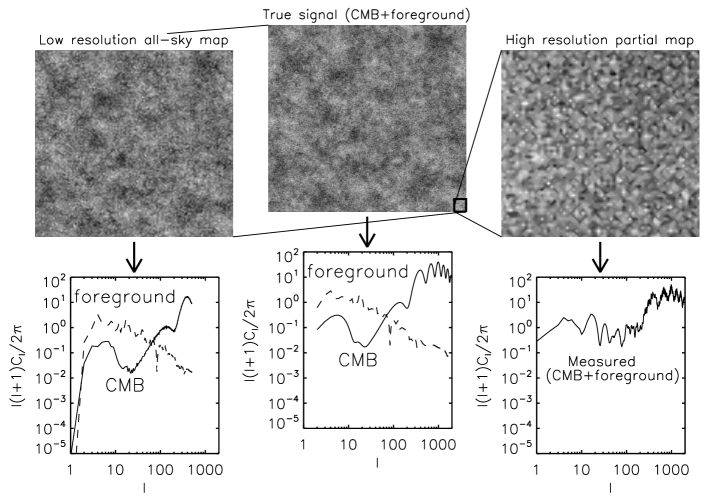
Figure 7.— Explanation of our filtering process. We use a Cartesian coordinate system for simplicity and assume there is only one foreground. Left panels: Low angular resolution all-sky map ($1024\times 1024$ pixels; $\Delta\theta\sim 21^{\prime}$). We generate the low resolution map by applying a circular top-hat filter on the data shown in the middle panels. The radius of the filter is 4 grid units, which is equivalent to $\sim 10.5^{\prime}$ The size of the resulting data file is $1024\times 1024$, the angular resolution of which corresponds to $\Delta\theta\sim 21^{\prime}$. We obtain the spectra in the lower-middle panel by direct Fourier transform. Middle panels: All-sky map of the CMB and the foreground signals and their angular spectra. We generate the map in the upper-middle panel using the spectra shown in lower-middle panel. The actual resolution of the map we use for the calculation is $8192\times 8192$. Right panels: High angular resolution partial-sky map ($128\times 128$ pixels; $\Delta\theta\sim 5.2^{\prime}$). This data file is from the low-right corner of the original $8192\times 8192$ data. We obtain this map by skipping every other point in each direction, so that the angular resolution of this data ($\Delta\theta\sim 5.2^{\prime}$) is twice worse than the original $8192\times 8192$ data, but 4 times better than the low-resolution data in middle panels. On the original data file (i.e. on the $8192\times 8192$ data), the region spans $256\times 256$ grid points. Therefore, the size of the partial-sky map is $128\times 128$. The angular size of map in the upper-right panel is $11^{\circ}\times 11^{\circ}$. The maps shown in this figure are degraded to reduce file size.

Figure 8.— Angular spectrum of CMB obtained from the filtering process. Top: The solid line is the spectrum obtained from the filtering process and the dotted line is the original CMB spectrum. Note that, since the high-resolution data span only $11^{\circ}\times 11^{\circ}$, the estimated angular spectrum for $l\lesssim 100$ is meaningless. Bottom: The solid line represents relative percentage error between the estimated CMB (solid curve) and the true CMB (dotted curve) spectra.

In this subsection, we demonstrate how the filtering process works. For simplicity we use a Cartesian coordinate system. For demonstration purposes, we consider the CMB EE spectrum (see the thin-solid line in Fig. 6b) and Galactic dust foreground for the case of stratified medium (see the dashed line in Fig. 6b).

Suppose that low-resolution all-sky maps are already available for many frequency channels. Let us assume the resolution of the maps is $\Delta\theta\sim 21^{\prime}$, which is similar to the WMAP resolution. Since there are many channels, one may use the usual filtering techniques to separate the CMB and the foreground signals. However, since we already know both the CMB and the foreground spectra in advance in this example, we do not follow the usual filtering techniques. Instead, we just assume that we already know the CMB and the foreground spectra for $l\lesssim 500$.

The ‘all-sky’ map in the upper-left panel of Figure 7 represents this low-resolution map. The map is defined on a grid of $1024\times 1024$ points. The angular resolution of the map is $\Delta\theta\sim 21^{\prime}$. We generate the map from a much higher-resolution all-sky map (see upper-middle panel), which has a dimension of $8196\times 8196$ in this example. When we obtain the low-resolution all-sky map from the much higher resolution all-sky map, we apply a circular top-hat beam pattern with radius $\sim 10.5^{\prime}$ to mimic actual observation. We calculate the spectra of the CMB and the foreground by direct Fourier transform of the low-resolution map data.

Then, suppose that we perform a high-resolution balloon experiment that can cover only part of the sky. In such balloon experiments, frequency channels are usually limited and removing foregrounds is a challenging task.

Here we show that, if we know the foreground spectrum, we can easily obtain the CMB spectrum from the balloon data. The upper-right panel of Figure 7 represents the high-resolution balloon data. The size of the data is $128\times 128$. The angular resolution is $\Delta\theta\sim 5.2^{\prime}$ and the map covers $11^{\circ}\times 11^{\circ}$ in the sky. We obtain the map by skipping every other point in each direction on low-right corner of the original map with $8192\times 8192$ points.

Our goal is to obtain the angular spectrum of the CMB signal using the balloon data. We first make the balloon data periodic by proper reflections and translations and obtain a periodic data on a grid of $4096\times 4096$ points. Then we multiply the data by a Gaussian profile of width $\sim 11^{\circ}$. The center of the Gaussian profile should locate near the center of the newly constructed $4096\times 4096$ pixel data and coincide with the center of a $128\times 128$ pixel original data. Then, we perform Fourier transform of the resulting data of size $4096\times 4096$. This way, we obtain an angular spectrum of the total (i.e. CMB+foreground) fluctuations.

Now, it is time to derive an angular spectrum of the foreground. We first take the angular spectrum from the low-resolution map, which is already available (see lower-left panel of Figure 7). The dashed curve is the foreground spectrum. The foreground spectrum is not defined for $l\gtrsim 500$. In principle, we know the foreground spectrum when we know geometry and turbulence spectrum. Here, we simply assume that the spectrum for $l\gtrsim 500$ is Kolmogorov. This way, we can construct the foreground spectrum for all values of $l$.

The remaining task is just subtraction: when we subtract the foreground spectrum from that of the total fluctuations, we can get the CMB spectrum. The solid curve in Figure 8 is the CMB spectrum obtained this way. The solid curve show a very good agreements with the original CMB spectrum used for generating the original all-sky data on a grid of $8192\times 8192$ points (see middle panels). The r.m.s. relative percentage error ($100\Delta C_{l}/C_{l}^{CMB}$) for $100<l<2000$ is 24%, where $\Delta C_{l}$ is the difference between the estimated CMB spectrum ($C_{l}^{estimated}$; solid curve) and the true CMB spectrum ($C_{l}^{CMB}$; dotted curve).

Note that the foreground spectrum depends on geometry of the emitting regions and underlying turbulence spectrum. In earlier sections, we discussed geometry of light-emitting regions. The turbulence spectrum may have some uncertainties (see Introduction). Kolmogorov spectrum may be good for a number of cases. However, it is possible that the spectrum deviated from Kolmogorov one in some regions, such as molecular clouds. However, such deviation will not affect our filtering process much if the resolution of balloon data is not far beyond that of the low-resolution all-sky map.

5.4. Demonstration of the filtering technique 2

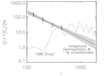
Figure 9.— Second demonstration of the spatial filtering technique. For demonstration purposes, the foreground signal has been enhanced by 1000 times. Left: Most-likely foreground spectrum (solid line) and its $1\sigma$ uncertainties (shaded region). We obtain the spectrum and the uncertainties using the observed data. In this example, we mark the 4 observed point with error bars. See the text for details. Right: CMB spectrum obtained from the spatial filtering technique. It shows that the spatial filtering technique works for $l\gtrsim 550$, where the CMB and the foreground spectra have similar values. This result implies that the technique will work when the CMB spectrum is slightly larger than the foreground one.

In the previous subsection, we demonstrated a reconstruction of CMB spectrum. The result is very promising because the dust foreground model we used is not far from a realistic one. Note that we normalized the amplitude of the dust foreground spectrum using the value quoted in an earlier work (Page et al. 2007).

However, there are a couple of issues regarding to the previous demonstration. First, in the previous demonstration, we assumed that we know the exact power-law index of the foreground spectrum. In general, we may not know the exact power-law index of the foregrounds. When this is the case, we need to extrapolate the foreground spectrum to larger values of multipoles and figure out to what extent we can safely extrapolate. Second, it is necessary to test how well our method works when the CMB and the foreground spectra are comparable.

In this subsection, we develop a method of deriving a most probable extrapolation of the foreground spectrum. We also test the performance of our technique for the case the CMB and the foreground spectra are comparable. For this purpose, we scale up the amplitude of the foreground spectrum by a factor of 1000.

As in the previous subsection, we assume that multi-channel observations are available for $l\lesssim 500$. Therefore, we have foreground observation for $l\lesssim 500$. However, unlike the previous subsection, we assume that observations are available only for selected values of multipole $l$. We mark 4 such $l$ values on Fig. 9. We use the same foreground spectrum as in the previous subsection to generate the 4 observed points. We also show the $1\sigma$ observation error bars for them, which are arbitrarily assigned in this example.

Using the 4 observed points for foreground, we find the most probable extrapolation for $l>500$. It is tempting to use the linear least-square fit in a $\log$-$\log$ plane, in which x-axis is a logarithm of $l$ and y-axis is that of $l(l+1)C_{l}/2\pi$. But, it is not easy to estimate uncertainties in this case.

Therefore, we adopt a slightly different method. We work on the $\log$-$\log$ plane. In this subsection, we use the following conventions: $x\equiv\log l$, $y\equiv\log[l(l+1)C_{l}/2\pi]$ and $(x_{i},y_{i})$ ($i=1,...,N$, where $N=4$ in this example) denotes an observed point. For a given $x$, we want to find the most probable value and $1\sigma$ uncertainty of $y$. In order to find them, we follow the following procedure. First, we select an arbitrary $y$ and consider all possible lines that pass through $(x,y)$. Let the slope of such a line be $a$ and the y-intercept be $b$. Then, we calculate the following probability for the chosen $y$:

$$P(y)\equiv\exp\left[-\sum_{i=1}^{N}\frac{(y_{i}-z_{i})^{2}}{2\sigma_{i}^{2}}\right],$$ (25)

where $z_{i}=ax_{i}+b$ and $\sigma_{i}$ is the $1\sigma$ observation error for $i$. Second, we repeat similar calculations for different values of $y$. Third, we find the value of $y$ where $P_{tot}(y)\equiv\sum_{alllines}P(y)$ has the maximum. Fourth, we find $1\sigma$ of the distribution $P_{tot}(y)$. Fifth, we repeat similar calculations for different values of $x$.

We plot the result of this procedure in Fig. 9(a). The solid line denotes the most probable values of ‘$y$’ and the shaded region represents the $1\sigma$ uncertainty. The $1\sigma$ uncertainty gets larger as $l$ gets larger when $l>500$. Therefore, it may not be a good idea to extrapolate for $l$’s an order of magnitude larger than $500$ which is the maximum $l$ of the low-resolution multi-channel maps in our current example. However, it seems to be OK to extrapolate for $l$’s a few times larger than $500$ in our current example. We can reduce the $1\sigma$ uncertainty by reducing the observation error bars, which may enable us to extrapolate further for larger $l$’s.

As in the previous subsection, we subtract the most-likely foreground spectrum from the observed (i.e. CMB+foreground) spectrum. We plot the result in Fig. 9(b).

Fig. 9(b) shows that our technique recovers the CMB spectrum quite well for $l\gtrsim 550$. Note that Fig. 9(a) tells us that the CMB and the foreground signals are almost same at $l\sim 550$. This example implies that our technique works when the CMB spectrum is slightly larger than the foreground spectrum. It is not likely that our technique in the current form works if the foreground spectrum is larger than the CMB one. However, even in this case, it is possible that our technique can help to reduce observational uncertainties when combined with conventional multi-channel methods.

The spatial filtering that we advocate here may be used as a part of a more general filtration procedure which uses both spatial and frequency information. Indeed, it is well recognized that the studies of tensor B-modes provide an excessively severe challenge to the precision of the removal of foregrounds. In this situation, it is important to reduce the errors of the determination of the foreground signal. The customarily used frequency templates provide filtering which is limited by both systematic and measurement errors. In this situation, any additional information helping to decrease the errors is highly valuable. The spatial power spectrum of the fluctuations that we discussed in the paper does provide such an information. This approach can be illustrated with Figure 9, which currently has only points for low $l$. However, it is already can be seen that the initial error bars of the points can be decreased if we require that the points correspond to a power-law spectrum. If we had more points at higher $l$ it is evident that the uncertainties could be further reduced. In other words, the constraint that the foreground fluctuations follow power law allows us to partially remove foregrounds at scales at which no foreground templates based on multi-frequency measurements are available and, at the same time, increase the precision of the foreground removal if the templates are available.

6. Discussion

6.1. Our approach

The major claim in this paper is that the statistical regularity of the foreground fluctuations enables one to extend their spectra from the scales where observations are available to the scales with no observations. In other words, the spatial spectra of foregrounds are predictable. This, in its turn, makes possible spatial filtering of foregrounds.

The predictability of Galactic foreground fluctuations stems from the fact that they are due to ubiquitous Galactic turbulence. MHD turbulence is known to have well-defined statistical properties both in compressible and incompressible limits (see Cho & Lazarian 2005 for a review). Thus one expects to see power-law behavior, which in the case of magnetic field is expected to correspond to 3D power spectrum close to the Kolmogorov one. In the case of density, the spectrum is Kolmogorov for the subsonic turbulence, but gets shallower than the Kolmogorov one for supersonic turbulence (see §4.1). Irrespectively of the underlying 3D spectrum being Kolmogorov or not we claim that one can predict the entire spectrum of spatial 2D foreground fluctuations, when the measurements over a limited range of scales are available. For this purpose we need to know the geometric properties of the volume. Our expectations of the underlying spectrum to be in some instances, e.g. for magnetic field, to be close to Kolmogorov only help to increase the accuracy of our prediction of the 2D foreground spectrum.

With the 2D predicted spectrum one then can use the procedure of filtering the foreground using Eq. (2) (see §5.3 for demonstration of the procedure). Alternatively, the good correspondence of the observed spatial spectrum of the foregrounds may serve as an additional proof of the accuracy of the foreground removal procedure. Needless to say, the information of the Galactic turbulence and the geometry of the emitting region that can be a by-product of the CMB research is of astrophysical significance.

A note of warning is due, however. The procedure of statistical filtering that we demonstrated in the paper, as any other procedure of the foreground removal, is not ideal. The power-law approximation of $C_{l}^{F}$ is definitely not exact. In this paper we have analyzed the causes for such deviations and provided the explanation for most notable features characterizing the change. More detailed modeling of Galactic turbulence is required.

6.2. Our data analysis

In this paper, we have discussed angular spectra of Galactic foregrounds. We have focused on synchrotron total intensity and polarized thermal dust emission. Our current study, as well as earlier studies (Chepurnov 1999; CL02), predicts that $C_{l}$ will reveal true 3D turbulence spectrum on small angular scales.

Our model calculations that take into account stratification effects imply that

1. $\theta<$ a few times $0.1^{\circ}$ (or $l>$ a few times $100$) for synchrotron emission (see Fig. 3), and

2. $\theta\lesssim 0.1^{\circ}$ (or $l\gtrsim 1000$) for polarized emission from thermal dust (see Fig. 6).

On larger angular scales, spectra are expected to be shallower.

6.3. Results

In this paper, we have analyzed Haslam 408MHz map and a model dust emission map and compared the results with model calculations. We have found that

1. The Haslam map for high Galactic latitude ($b>30^{\circ}$) can be explained by MHD turbulence in the Galactic halo. The measured second-order angular structure function is proportional to $\theta^{1.2}$, which corresponds to an angular spectrum of $l^{-3.2}$. The high-order statistics for high Galactic latitude ($b>30^{\circ}$) is consistent with that of incompressible magnetohydrodynamic turbulence. Our model calculations show that a two-component model (see §3.3 and Fig. 3) can naturally explain the observed angular spectrum. The one-component model can also explain the observed slope. But, the slope of the spectrum shows a more abrupt change near $l\sim 30$.

2. The model dust emission map may not have anything to do with turbulence on large angular scales. That is, we do not find signatures of turbulence in the map.

3. Both maps show flat high-order structure functions for the Galactic plane. This kind of behavior is expected when discrete structures dominate the map.

We have described how we can obtain angular spectrum of polarized emission from thermal dust in high Galactic latitude regions. Our model calculations show that starlight polarization arising from dust in high Galactic latitude regions will have a Kolmogorov spectrum, $C_{l}\propto l^{-11/3}$, for $l\gtrsim 1000$ and a shallower spectrum for $l\lesssim 1000$ (Fig. 6). We expect that polarized emission from the same dust also has a similar angular spectrum. That is, we expect that the angular spectrum of polarized emission from thermal dust is close to a Kolmogorov one for $l\gtrsim 1000$.

We have described a new technique of filtering CMB foregrounds. When we have

1. low angular resolution full-sky measurements (such as WMAP data) and

2. high angular resolution partial-sky measurements with limited frequency channels,

we can use the technique to derive the CMB angular spectrum for the high-resolution data. In §5.3 and §5.4, we have demonstrated the technique.

6.4. Comparison with approaches in the literature

The existing confusion in the literature include naive identification of the 2D spectra of foregrounds with the spectra of the underlying fluctuations. Therefore, for instance, from the fact that the spectral slope of $C_{l}^{F}$ differ from the Kolmogorov one, the conclusion about the nature of the fluctuations is made.

In the paper above we have shown that the 2D spectra may have a spectral slope different from the underlying spectral slope of the turbulence. We showed that it is essential to take into account the non-trivial geometry of observations with the observer sampling turbulence along the diverging lines of sight and within the volume where the density of emitters changes. For the case of the synchrotron fluctuations we showed that the observed non-Kolmogorov value of the spectral index of $C_{l}^{F}$ can be reconciled with the Kolmogorov-type turbulence.

A notable difference of our study compared with CL02 is that in the latter study we tried to necessarily associate the spectra of foregrounds with the underlying Kolmogorov or Goldreich-Sridhar (1995) turbulence with the spectral slope $-11/3$. The limitations of these approach get evident in view of establishing of the shallow spectral index of density fluctuations in supersonic MHD turbulence (Beresnyak et al. 2005). These fluctuations, according to our present study, can explain the observed spectra of Galactic dust emission.

6.5. Limitations and extensions of our filtering procedure

The procedure of spatial statistical filtering discussed in §2 is very simplified. It should provide satisfactory results for a simple power law behavior of $C_{l}^{F}$ (see Figure 2). In more complex cases detailed modeling of the emitting volume and/or use of the filtering as a part of a more sophisticated foreground removal procedure is required. We partially addressed this issue in §5. Especially in §5.4, we described a method to estimate uncertainties stemming from a power-law modeling of the foreground spectrum. Nevertheless, more improvement is needed for the new technique. At the same time, we believe that our approach can be applied to the removal of foregrounds not only from the CMB data, but, for instance, from the high-$z$ hydrogen statistics studies.

7. Summary

In the paper above we have obtained the following results:

1. We provided additional evidence that the synchrotron Galactic emissivity is consistent with the halo + disk model. Within this model we show that the spatial spectrum of the underlying 3D fluctuations is consistent with the Kolmogorov one.

2. Within our model we related the angular scale for the change of the power spectrum of the synchrotron fluctuations with the ratio of the injection scale to the thickness of the observed region in the direction of observation.

3. We explained the spectrum of dust foreground emission as arising from the shallow spectrum of density fluctuations which characterizes supersonic MHD turbulence.

4. We used numerical modeling of grain optical properties to relate the polarization of starlight with the expected sub-mm foreground polarization and outlined the ways of quantitative use of starlight polarization maps to study sub-mm polarized dust foreground. We evaluated the uncertainty of the evaluated sub-mm polarization spectrum arising from the variations of the magnetic field direction in respect to the line of sight.

5. We showed that for randomly chosen sample of stars the spectrum of the starlight polarization for the underlying Kolmogorov turbulence depended on how the selected stars are distributed along the line of sight. For stratified model of Galactic dust we predicted the spectrum of spatial fluctuations with the index approaching the Kolmogorov value of $-11/3$ for $l>1000$.

6. On the basis of our improved understanding of the self-similar nature of the underlying MHD turbulence we proposed and tested a procedure of spatial statistical removal of Galactic foregrounds based on extending of the $C_{l}^{F}$ spectrum to higher $l$.

7. We studied the higher order correlations of the Galactic dust and synchrotron foregrounds and reported substantial difference with the higher-order scalings (see Appendix D). The synchrotron scaling shows intermittencies similar to magnetic fields in incompressible fluids, while dust scaling is closer to the intermittency demonstrated by highly compressible MHD turbulence.

Appendix A Spectrum and Structure Function of Diffuse Synchrotron Emission: a model for homogeneous turbulence revisited

Suppose that 3-dimensional (3D) MHD turbulence has a 3D spatial power spectrum of the form $E_{3D}\propto k^{-m}$, where $k$ is the wavenumber. Note that in Kolmogorov turbulence $m=11/3$. Then what will be the 2-dimensional angular spectrum, $C_{l}$, of the observed synchrotron total intensity? We cannot not directly observe the 3D spatial power spectrum. However, we can infer the 3D spectrum from the observed 2-dimensional (2D) angular spectrum, $C_{l}$, of the synchrotron total intensity. Then let us find out how the 3D spectrum, $E_{3D}(k)$, and the 2D angular spectrum, $C_{l}$, are related. We mostly follow discussions in Cho & Lazarian (CL02). We also make use of an analytical insight obtained in Lazarian (1992, 1995ab) and numerical results obtained in CL02. Although we focus on synchrotron emission here, the discussion in this section can be applicable to any kind of emission from an optically thin medium.

A.1. MHD turbulence and synchrotron emission

For synchrotron radiation, emissivity at a point ${\bf r}$ is given by $\epsilon({\bf r})\propto n(e)|{B}_{\bot}|^{\gamma}$, where $n(e)$ is the electron number density, $B_{\bot}$ is the component of magnetic field perpendicular to the line of sight. The index $\gamma$ is approximately $2$ for radio synchrotron frequencies (see Smoot 1999). If electrons are uniformly distributed over the scales of magnetic field inhomogeneities, the spectrum of synchrotron intensity reflects the statistics of magnetic field. For small amplitude perturbations ($\delta b/B\ll 1$; this is true for scales several times smaller than the outer scale of turbulence if we interpret $B$ as local mean magnetic field strength and $\delta b$ as random fluctuating field in the local region), if $\delta b$ has a power-law behavior, the synchrotron emissivity will have the same power-law behavior (see Getmantsev 1959; Lazarian & Shutenkov 1990; Chepurnov 1999). Therefore, we expect that the angular spectrum of synchrotron intensity also reflects the spectrum of 3-dimensional MHD turbulence.

When an observer is located inside a turbulent medium, the angular correlation function, hence the power spectrum, shows two asymptotic behaviors. When the angle is larger than a critical angle, we can show that the angular correlation shows a universal $\theta^{-1}$ scaling. On the contrary, when the angular separation is smaller than the critical angle, the angular correlation reflects statistics of turbulence. In this small angle limit, we can show that the angular power spectrum is very similar to that of turbulence. The critical angle is determined by the geometry. Let the outer scale of turbulence be $L$ and the distance to the farthest eddies be $d_{max}$. Then the critical angle is

$$\theta\sim L/d_{max}.$$ (A1)

A.2. Small-angle limit in homogeneous turbulence

When the angle between the lines of sight is small (i.e. $\theta<L/d_{max}$), the angular spectrum $C_{l}$ has the same slope as the 3-dimensional energy spectrum of turbulence. Lazarian & Shutenkov (1990) showed that if the 3D spatial spectrum of a variable follows a power law, $E_{3D}(k)\propto k^{-m}$, then the 2-dimensional spectrum of the variable projected on the sky also follows the same power law,

$$C_{l}\propto l^{-m}$$ (A2)

in the small $\theta$ limit. For Kolmogorov turbulence ($E_{3D}\propto k^{-11/3}$), we expect

$$C_{l}\propto l^{-11/3},\mbox{~{}~{}~{}if $\theta<L/d_{max}$.}$$ (A3)

Note that $l\sim\pi/\theta$.

In some cases, when we have data with incomplete sky coverage, we need to infer $C_{l}$ from the observation of the angular correlation function

$$w(\theta)=<I({\bf e}_{1})I({\bf e}_{2})>,$$ (A4)

where $I({\bf e})$ is the intensity of synchrotron emission, ${\bf e}_{1}$ and ${\bf e}_{2}$ are unit vectors along the lines of sight, $\theta$ is the angle between ${\bf e}_{1}$ and ${\bf e}_{2}$, and the angle brackets denote average taken over the observed region. As we discuss in Appendix A, when the underlying 3D turbulence spectrum is $\propto k^{-m}$ (e.g. $m=11/3$ for Kolmogorov turbulence), the angular correlation function $w(\theta)$ is given by

$$w(\theta)~{}\propto~{}<I^{2}>-\mbox{const}~{}\theta^{m-2},\mbox{~{}~{}~{}if $\theta<L/d_{max}$.}$$ (A5)

It is sometimes inconvenient to use the angular correlation function in practice to study turbulence statistics because of the constant $<I^{2}>$.

A better quantity in small-angle limit would be the second-order angular structure function:

$$D_{2}(\theta) = <|I({\bf e}_{1})-I({\bf e}_{2})|^{2}>$$ (A6)

$$= 2<I^{2}>-2w(\theta).$$ (A7)

Thus, in homogeneous turbulence with 3D spatial spectrum of $E(k)\propto k^{-m}$, we have

$$D_{2}(\theta)\propto\theta^{m-2}.$$ (A8)

When we measure the slope of the angular structure function, we can infer the slope of the 3D spatial power spectrum of turbulence.

Figure 10.— Two limits in homogeneous turbulence. Upper plot: Small $\theta$ limit ($\theta<L/d_{max}$). The fluctuations along the entire length of the lines of sight are correlated. Lower plot: Large $\theta$ limit ($\theta>L/d_{max}$). Only points close to the observer are correlated. Note the definition of $r$ and $\psi$. From CL02.

A.3. Large-angle limit in homogeneous turbulence

In this limit, the angular correlation function is more useful than the structure function. Following Lazarian & Shutenkov (1990), we can show that the angular correlation function for $\theta>L/d_{max}$ follows

$$w(\theta) = \int\int dr_{1}dr_{2}~{}{\cal K}(|{\bf r}_{1}-{\bf r}_{2}|),$$ (A9)

$$= \frac{1}{\sin{\theta}}\int_{0}^{\infty}dr~{}r{\cal K}(r)\int_{\theta/2}^{\pi-\theta/2}d\psi\propto\frac{\pi-\theta}{\sin\theta}\sim\frac{const}{\theta},$$

where ${\cal K}(r)$ is the 3D spatial correlation function and we change variables: $(r_{1},r_{2})\rightarrow(r,\psi)$, which is clear from Fig. 10. We accounted for the Jacobian of which is $r/\sin{\theta}$. We can understand $1/\theta$ behavior qualitatively as follows. When the angle is large, points along of the lines-of-sight near the observer are still correlated. These points extend from the observer over the distance $\propto 1/\sin{(\theta/2)}$.

If we assume $L/d_{max}<\theta\ll 1$, we can get the angular power spectrum $C_{l}$ using Fourier transform:

$$C_{l} \sim \int\int w(\theta)e^{-i{\bf l}\cdot{\bf\theta}}d\theta_{x}d\theta_{y}$$ (A10)

$$\sim \int d\theta~{}\theta J_{0}(l\theta)w(\theta)\propto l^{-1},$$

where $\theta=(\theta_{x}^{2}+\theta_{y}^{2})^{1/2}$, $J_{0}$ is the Bessel function, and we use $w(\theta)\propto\theta^{-1}$.

A.4. Expectations for homogeneous turbulence

In summary, for homogeneous Kolmogorov turbulence (i.e. $E(k)\propto k^{-11/3}$), we expect from equations (A3) and (A10) that

$$C_{l}\propto\left\{\begin{array}[]{ll}l^{-11/3}&\mbox{if $l>l_{cr}$}\\ l^{-1}&\mbox{if $l<l_{cr}$,}\end{array}\right.$$ (A11)

which means that the power index $\alpha$ of $C_{l}$ is $-1\leq\alpha\leq-11/3$. We expect the following scaling for the second-order angular structure function:

$$D_{2}(\theta)\propto\left\{\begin{array}[]{ll}\theta^{5/3}&\mbox{if $\theta<L/d_{max}$ }\\ \mbox{constant}&\mbox{if $\theta>L/d_{max}$.}\end{array}\right.$$ (A12)

The critical angle $\theta_{cr}\sim L/d_{max}$ depends on the size of the large turbulent eddies and on the length of the line of sight. If we assume that turbulence is homogeneous along the lines of sight and has $L\sim 100\ pc$ corresponding to a typical size of the supernova remnant, and that $d_{max}\sim 1$ kpc for synchrotron halo (see Smoot 1999), we get $\theta_{cr}\sim 6^{\circ}$.

Appendix B The second-order angular structure function in the small angle limit

In this Appendix, we discuss how underlying 3D statistics and observed 2D statistics are related. This discussion is useful when we infer 3D statistics from observed 2D statistics, or vice versa. Strictly speaking, discussion in the section is applicable to homogeneous and isotropic turbulence only.

The angular correlation $w(\theta)$ is given by the integral

$$w(\theta)=\int dl_{1}\int dl_{2}~{}{\cal K}(|{\bf l}_{1}-{\bf l}_{2}|),$$ (B1)

where ${\cal K}(r)$ is the 3 dimensional spatial correlation. Suppose that ${\bf l}_{1}$ is along x-axis, ${\bf l}_{1}=(l_{1},0)$, and ${\bf l}_{2}=l_{2}(\cos\theta,\sin\theta)$. Then, the correlation in the limit of small $\theta$ is given by

$$w(\theta) = \int dl_{1}\int dl_{2}~{}{\cal K}\left(\sqrt{(l_{1}-l_{2}\cos\theta)^{2}+l_{2}^{2}\sin^{2}\theta}\right)$$ (B2)

$$= \int dl_{1}\int dl_{2}~{}{\cal K}\left(\sqrt{(l_{1}^{2}-2l_{1}l_{2}\cos\theta+l_{2}^{2}}\right)$$ (B3)

$$\approx \int dl_{1}\int dl_{2}~{}{\cal K}\left(\sqrt{(l_{1}-l_{2})^{2}+l_{1}l_{2}\theta^{2}}\right).$$ (B4)

Suppose that the spatial correlation follows a power law: ${\cal K}(r)\propto\mbox{~{}const}-r^{p}$ for $r<L$, where $L$ is the outer-scale of turbulence. For Kolmogorov turbulence, $p=2/3$. Then the derivative of $w(\theta)$ is given by

$$\frac{w(\theta)}{d\theta} \propto -\int dl_{1}\int dl_{2}~{}\left[(l_{1}-l_{2})^{2}+l_{1}l_{2}\theta^{2}\right]^{p/2-1}(2l_{1}l_{2}\theta)$$ (B5)

$$-\propto \int du\int dw~{}\left[w^{2}+(u^{2}-w^{2})\theta^{2}/4\right]^{p/2-1}(u^{2}-w^{2})\theta/2,$$ (B6)

where $u=l_{1}+l_{2}$ and $w=l_{1}-l_{2}$. If $p\leq 1$, the integration diverges as $\theta$ goes to zero. Therefore, when $p\leq 1$, it suffices to perform the integration in the vicinity of $l_{1}=l_{2}$ or $w=0$. Then we have

$$\frac{w(\theta)}{d\theta} \propto -\int du\int dw~{}\left[w^{2}+u^{2}\theta^{2}/4\right]^{p/2-1}u^{2}\theta/2$$ (B7)

$$\approx -\int du~{}(u\theta/2)^{p-1}u^{2}\theta/2\propto-\theta^{p},$$ (B8)

where we use $\int_{-\infty}^{+\infty}dw/(w^{2}+A^{2})^{n}=A^{1-2n}\int_{-\pi/2}^{+\pi/2}d\theta~{}\sec^{2-2n}\theta$. Therefore, for small $\theta$ we have

$$w(\theta)\propto C_{1}-C_{2}\theta^{p+1},$$ (B9)

where $C_{1}$ and $C_{2}$ are constants. Comparing this equation with

$$w(\theta)=\mbox{$C_{3}$}-C_{4}D_{2}(\theta),$$ (B10)

we get

$$D_{2}(\theta)\propto\theta^{p+1}.$$ (B11)

Analytic expressions for the relation between the angular structure function ($D_{2}$) and the spatial 1D spectrum (E(k); in case of Kolmogorov, $E(k)\propto k^{-5/3}$) can be found in the literature. For example, Lazarian (1995a; see also Lazarian & Shutenkov 1990) derived the following expression:

$$E(k)\propto k\int_{0}^{{\cal L}/R}d\eta~{}\frac{d}{d\eta}\left(Q(\eta)\eta\right)J_{1}(kR\eta)+{\cal K}_{5},$$ (B12)

where ${\cal L}$ can be regarded as the outer scale of turbulence, $R$ is the size of the system, $Q(\eta)\sim D_{2}^{\prime}(\eta)\eta$, $\eta=\sin\theta$, $J_{1}(x)$ is the Bessel function of the first order, and ${\cal K}_{5}$ is a small correction term.

Appendix C Spatial spectrum of emissivity

The synchrotron emissivity is proportional to $\sim n(e)B^{\gamma}\propto B^{2}$, where $n(e)$ is the high-energy electron number density. Suppose that magnetic field is roughly a Gaussian random variable. This may not be exactly true, but should be a good approximation. When a Gaussian random variable $B({\bf r})$ follows a Kolmogorov spectrum

$$E_{B,3D}\equiv|\tilde{B}(k)|^{2}\propto\left\{\begin{array}[]{ll}0&\mbox{if $k\leq k_{0}$}\\ (k/k_{0})^{-11/3}&\mbox{if $k\geq k_{0}$,}\end{array}\right.$$ (C1)

we can show that the 3D spectrum of $B^{2}(r)$ follows Eq. 9 (see, for example, Chepurnov 1999). The correlation of $B^{2}(r)$ and 3D energy spectrum of $B^{2}(r)$ are related by

$${\cal K}_{B^{2}}({\bf r})=<B^{2}({\bf x})B^{2}({\bf x}+{\bf r})>_{x}\propto\int E_{B^{2},3D}({\bf k})e^{i{\bf k}\cdot{\bf r}}d^{3}{\bf k},$$ (C2)

$$E_{B^{2},3D}({\bf k})\equiv|\tilde{B^{2}}(k)|^{2}\propto\int{\cal K}_{B^{2}}({\bf r})e^{-i{\bf k}\cdot{\bf r}}d^{3}{\bf r},$$ (C3)

where $<...>_{x}$ denotes an average over ${\bf x}$. A Gaussian random variable satisfies

$$<B^{2}({\bf x})B^{2}({\bf x}+{\bf r})>=<B^{2}({\bf x})><B^{2}({\bf x}+{\bf r})>+2<B({\bf x})B({\bf x}+{\bf r})>^{2},$$ (C4)

where the first term on the right is a constant. Therefore we can ignore the term in what follows. Fourier transform of both sides results in

LHS $$= E_{B^{2},3D}({\bf k}),$$ (C5)

RHS $$= 2\int<B({\bf x})B({\bf x}+{\bf r})>^{2}e^{-i{\bf k}\cdot{\bf r}}d^{3}{\bf r}$$ (C6)

$$= 2\int~{}d^{3}{\bf r}~{}{\cal K}_{B}({\bf r})~{}{\cal K}_{B}({\bf r})e^{-i{\bf k}\cdot{\bf r}}$$ (C7)

$$= 2\int~{}d^{3}{\bf r}\int~{}d^{3}{\bf p}\int~{}d^{3}{\bf q}~{}E_{B,3D}({\bf p})E_{B,3D}({\bf q})e^{i({\bf p}+{\bf q}-{\bf k})\cdot{\bf r}}$$ (C8)

$$= 2\int~{}d^{3}{\bf p}\int~{}d^{3}{\bf q}~{}E_{B,3D}({\bf p})E_{B,3D}({\bf q})\delta({\bf p}+{\bf q}-{\bf k})$$ (C9)

$$= 2\int~{}d^{3}{\bf p}~{}E_{B,3D}({\bf p})~{}E_{B,3D}({\bf k}-{\bf p}),$$ (C10)

where $\delta(k)$ is the Dirac $\delta$-function. Therefore we have

$$E_{B^{2},3D}({\bf k})\approx E_{B^{2},3D}({\bf 0})\approx 2\int~{}d^{3}{\bf k}|E_{B,3D}({\bf k})|^{2}\approx\mbox{constant}$$ (C11)

for $k\ll k_{0}$.

Appendix D High-order statistics

While most of the paper is directly related to making use of the knowledge of the underlying spectra and/or two points correlations in order to remove foregrounds, the part dealing with higher-order statistics is not directly related to the foreground removal. Nevertheless, the correspondence of the intermittencies of foregrounds to those of turbulence provide another support for our understanding of the turbulent origin of foreground fluctuations.

High-order structure functions are used for the study of intermittency, which refers to the non-uniform distribution of structures. Since CMB signals are close to Gaussian, one may think that they do not have strong intermittency. However, there is a report that intermittency of CMB signals deviate from Gaussianity (Bershadskii & Screenivasan 2003). If intermittency of foreground signals are different from that of CMB signals, we can potentially use high-order structure functions to separate CMB and foreground signals. In addition, we can use high-order structure functions to improve our knowledge of foregrounds.

The structure functions of order $p$ for an observable $I$ is defined by

$$S_{p}(r)=<|I(x)-I(x+r)|^{p}>,$$ (D1)

where the angled brackets denote average over position $x$. For an observable defined in the plane of the sky, the angular structure function of order $p$ is

$$D_{p}(\theta)=<|I({\bf e}_{1})-I({\bf e}_{2})|^{p}>.$$ (D2)

Traditionally, researchers use high-order structure functions of velocity to probe dissipation structures of turbulence. In fully developed hydrodynamic turbulence, the (longitudinal) velocity structure functions $S_{p}=<([{\bf v}({\bf x}+{\bf r})-{\bf v}({\bf x})]\cdot\hat{\bf r})^{p}>\equiv<\delta v_{L}^{p}({\bf r})>$ are expected to scale as $r^{\zeta_{p}}$:

$$S_{p}(r)\propto r^{\zeta_{p}}.$$ (D3)

One of the key issues in this field is the functional form of the scaling exponents $\zeta_{p}$. There are several models for $\zeta_{p}$. Roughly speaking, the dimensionality of the energy dissipation structures plays an important role.

Assuming 1-dimensional worm-like dissipation structures, She & Leveque (1994) proposed a scaling relation

$$\zeta_{p}^{SL}=p/9+2[1-(2/3)^{p/3}]$$ (D4)

for incompressible hydrodynamic turbulence. Note that $\zeta_{p}$ is the scaling exponent of structure of order $p$. On the other hand, assuming 2-dimensional sheet-like dissipation structures, Müller & Biskamp (2000) proposed the relation

$$\zeta_{p}^{MB}=p/9+1-(1/3)^{p/3}$$ (D5)

for incompressible magneto-hydrodynamic turbulence.

Recently, high-order structure functions of molecular line intensities have been also employed (Padoan et al. 2003; Gustafsson et al. 2006). In optically thin case, the molecular line intensities are proportional to the column density. Kowal, Lazarian, & Beresnyak (2007) studied scaling of higher moments of density fluctuations in MHD turbulence. Their numerical results show that, first of all, the scalings of higher moments in 3D can be obtained by studying the distribution of column densities. Then, they showed that the behavior of the scaling exponents for column density depends on sonic Mach number of turbulence.

Bershadskii & Screenivasan (2003) calculated intermittency of CMB signals. Their result shows that the WMAP data follow She-Leveque scaling. Therefore, it is interesting to see if foreground signals show different scalings.

We plot the scaling exponents of the Haslam 408MHz map in Fig. 11. The Haslam map shows a reasonable agreement with the Muller-Biskamp MHD model. Note that Padoan et al. (2003) also obtained a similar result using ${}^{13}CO$ emission from Perseus and Taurus.

Unlike the Haslam map, the 94GHz dust map does not show agreement with Muller-Biskamp model. The scaling exponents do not show strong dependence on the order $p$ similar, which makes them similar to the results of the potential part of the supersonic flow studied in Kowal & Lazarian (2010) and densities in supersonic super-Alfvenic flows studied in Kowal et al. (2007). One may expect that in the presence of self-gravity this is what is expected for higher order statistics of density, but further studies are required.

Left and middle panels of Fig. 12 show that the slope is around 1 for high-order structure functions. This kind of behavior is expected when discrete structures dominate the map. However, it is not clear what kinds of discrete structures dominate. Since the Haslam map and the dust map sample different types of the ISM, it is not so surprising that they show different scaling behaviors.

For the Galactic disk, high-order structure functions of both maps show nearly flat structure functions. The structure functions show a nearly flat behavior down to $\theta\sim 1^{\circ}$, which happens to be the actual angular resolution of the maps. Further studies of MHD turbulence in the presence of self-gravity should clarify the origin of such behavior. Alternatively, higher moments of structure functions can be affected by unresolved point sources.

Figure 11.— High order statistics of the Haslam 408MHz map. Left: The second, third, 5th, and 8th-order structure functions for $b>30^{\circ}$. Middle: The scaling exponents for $b>30^{\circ}$ seem to follow the Muller-Biskamp MHD scaling. Note that we equate the scaling exponent of the observed third-order structure function and that of the Muller-Biskamp model (see more discussion in Cho et al. 2003). We measure the slope between $\theta=1^{\circ}$ and $10^{\circ}$. Right: The second, third, 5th, and 8th-order structure functions for the Galactic disk ($-2^{\circ}\leq b\leq 2\circ$). They are all flat.

Figure 12.— High order statistics of the 94GHz dust emission map. We use dust emission intensity times $\sin b$ for all calculations. Left: The second, third, 5th, and 8th-order structure functions for $b>30^{\circ}$. Middle: The scaling exponents for $b>30^{\circ}$ does not show signatures of turbulence. We measure the slope between $\theta=1^{\circ}$ and $10^{\circ}$. Right: The second, third, 5th, and 8th-order structure functions for the Galactic disk ($-2^{\circ}\leq b\leq 2\circ$). They are all flat.

References

- (1) Armstrong, J., Rickett, B., & Spangler, S. 1995, ApJ, 443, 209
- (2) Baccigalupi, C., Burigana, C., Perrotta, F., De Zotti, G., La Porta, L., Maino, D., Maris, M., & Paladini, R. 2001, A&A, 372, 8
- (3) Beuermann, K., Kanbach, G., & Berkhuijen, E. 1985, A&A, 153, 17
- Beresnyak & Lazarian (2006) Beresnyak, A., & Lazarian, A. 2006, ApJ, 640, L175
- Beresnyak & Lazarian (2009) Beresnyak, A., & Lazarian, A. 2009, ApJ, 702, 1190
- Beresnyak et al. (2005) Beresnyak, A., Lazarian, A., & Cho, J. 2005, ApJ, 624, L93
- (7) Bershadskii, A. & Screenivasan, K.R. 2003, Phys. Lett. A, 319, 21
- (8) Boldyrev, S. 2002, ApJ, 569, 841
- (9) Boldyrev, S. 2006, Phys. Rev. Lett., 96, 115002
- (10) Bouchet, F. & Gispert, R. 1999, New Astronomy, 4, 443
- (11) Bouchet, F., Gispert, R., & Pouget, J.-L. 1996, AIP Conf. Proc., No. 348, 255
- (12) Chepurnov, A. V. 1999, Astron.Astrophys.Trans. 17, 281, astro-ph/0206407
- Chepurnov & Lazarian (2009) Chepurnov, A., & Lazarian, A. 2009, ApJ, 693, 1074
- Chepurnov & Lazarian (2010) Chepurnov, A., & Lazarian, A. 2010, ApJ, 710, 853
- Chepurnov et al. (2006) Chepurnov, A., Lazarian, A., Stanimirovic, S., Heiles, C., & Peek, J. E. G. 2010, ApJ, in press (arXiv:astro-ph/0611462)
- (16) Cho, J. & Lazarian, A. 2002a, ApJ, 575, 63 (CL02)
- Cho & Lazarian (2002) Cho, J., & Lazarian, A. 2002b, Physical Review Letters, 88, 245001
- Cho & Lazarian (2003) Cho, J., & Lazarian, A. 2003, MNRAS, 345, 325
- Cho & Lazarian (2005) Cho, J., & Lazarian, A. 2005, Theoretical and Computational Fluid Dynamics, 19, 127
- Cho et al. (2002) Cho, J., Lazarian, A., & Vishniac, E. T. 2002, ApJ, 564, 291
- Cho & Vishniac (2000) Cho, J., & Vishniac, E. T. 2000, ApJ, 539, 273
- (22) de Oliveira-Costa, A., Tegmark, M., O’dell, C., Keating, B., Timbie, P., Efstathiou, G., & Smoot, G. 2003, Phys. Rev. D, 68, 083003
- (23) Dolginov, A. Z., Gnedin, Iu. N., & Silantev, N. A. 1996, Propagation and Polarization of Radiation in Cosmic Media, (Gordon & Breech)
- (24) Draine, B. 1985, ApJS, 57, 587
- (25) Draine, B. & Lazarian, A. 1998a, ApJ, 494, 19
- (26) Draine, B. & Lazarian, A. 1998b, ApJ, 508, 157
- (27) Draine, B. & Lee, H. 1984, ApJ, 285, 89
- (28) Draine, B. & Flatau P. 1994, Opt. Soc. Am. A, 11, 1491
- (29) Draine, B. & Flatau P. 2008, arXiv:0809.0337
- Draine & Weingartner (1996) Draine, B. T., & Weingartner, J. C. 1996, ApJ, 470, 551
- Draine & Weingartner (1997) Draine, B. T., & Weingartner, J. C. 1997, ApJ, 480, 633
- Dunkley et al. (2009) Dunkley, J., et al. 2009, American Institute of Physics Conference Series, 1141, 222 (arXive:0811.3915)
- Elmegreen & Scalo (2004) Elmegreen, B. G., & Scalo, J. 2004, ARA&A, 42, 211
- Esquivel & Lazarian (2005) Esquivel, A., & Lazarian, A. 2005, ApJ, 631, 320
- Esquivel et al. (2007) Esquivel, A., Lazarian, A., Horibe, S., Cho, J., Ossenkopf, V., & Stutzki, J. 2007, MNRAS, 381, 1733
- Esquivel et al. (2003) Esquivel, A., Lazarian, A., Pogosyan, D., & Cho, J. 2003, MNRAS, 342, 325
- (37) Finkbeiner, D. P., Davis, M., & Schlegel, D. J. 1999, ApJ, 524, 867
- Finkbeiner et al. (2002) Finkbeiner, D. P., Schlegel, D. J., Frank, C., & Heiles, C. 2002, ApJ, 566, 898
- (39) Fowler et al. 2010, arXiv:1001.2934v1
- (40) Fosalba, P., Lazarian, A., Prunet, S., & Tauber, J.A. 2002 ApJ, 564, 762 (FLPT)
- Fuchs et al. (2008) Fuchs, B., Breitschwerdt, D., de Avillez, M. A., & Dettbarn, C. 2008, Space Science Reviews, 148
- (42) Getmantsev, G. 1959, Soviet Astronomy, 3, 415
- (43) Giardino, G., Banday, A. J., Bennett, K., Fosalba, P., Gorski, K. M., O’Mullane, W., Tauber, J., & Vuerli, C. 2001a, in Mining the Sky, ed. A. J. Banday, S. Zaroubi, & M. L. Bartelmann (Heidelberg: Springer), 458
- (44) Giardino, G., Banday, A. J., Fosalba, P., Gorski, K. M., Jonas, J. L., O’Mullane, W., & Tauber, J. 2001b, A&A, 371, 708
- (45) Giardino, G., Banday, A.J., Górski, K.M., Bennett, K., Jonas, J.L., & Tauber, J. 2002, A&A, 387, 82
- (46) Ginzburg, V. & Ptuskin, V. 1976, Rev. Mod. Phys. 48, 161
- Goldreich & Sridhar (1995) Goldreich, P., & Sridhar, S. 1995, ApJ, 438, 763
- (48) Górski, K., Hivon, E., Banday, A., et al. 2005, ApJ, 622, 759
- (49) Gustafsson, M., Brandenburg, A., Lemaire, J., & Field, D. 2006, A&A, 454, 815
- (50) Haslam, C., Salter, C., Stoffel, H., & Wilson, W. 1982, A&AS, 47, 1
- Haverkorn et al. (2008) Haverkorn, M., Brown, J. C., Gaensler, B. M., & McClure-Griffiths, N. M. 2008, ApJ, 680, 362
- (52) Heiles, C. 2000, AJ, 119, 923
- Hildebrand et al. (2009) Hildebrand, R. H., Kirby, L., Dotson, J. L., Houde, M., & Vaillancourt, J. E. 2009, ApJ, 696, 567
- (54) Hildebrand, R., Davidson, J., Dotson, J., Dowell, C., Novak, G., & Vaillancourt, J. 2000, PASP, 112, 1215
- (55) Hildebrand, R., Dotson, J., Dowell, C., Schleuning, D., & Vaillancourt, J. 1999, ApJ, 516, 834
- Hoang & Lazarian (2008) Hoang, T., & Lazarian, A. 2008, MNRAS, 388, 117
- Hoang & Lazarian (2009) Hoang, T., & Lazarian, A. 2009a, ApJ, 695, 1457
- Hoang & Lazarian (2009) Hoang, T., & Lazarian, A. 2009b, ApJ, 697, 1316
- (59) Jonas, J. L., Baart, E. E., & Nicolson, G. D. 1998, MNRAS, 297, 977
- Kim & Ryu (2005) Kim, J., & Ryu, D. 2005, ApJ, 630, L45
- (61) Kowal, G., Lazarian, A., & Beresnyak, A. 2007, ApJ, 658, 423
- (62) Kowal, G. & Lazarian, A. 2007, ApJL, 666, L69
- (63) Kowal, G. & Lazarian, A. 2010, ApJ, submitted
- (64) Lazarian, A. 1992, Astron. & Astrophys. Trans., 3, 33
- (65) Lazarian, A. 1995a, Ph. D. Thesis (Univ. of Cambridge, UK)
- (66) Lazarian, A. 1995b, A&A, 293, 507
- (67) Lazarian, A. 2007, J. Quant. Spectrosc. Radiat. Trans., 106, 225
- (68) Lazarian, A. 2009, Space Science Rev., accepted (arXiv:0811.0839)
- Lazarian & Esquivel (2003) Lazarian, A., & Esquivel, A. 2003, ApJ, 592, L37
- (70) Lazarian, A. & Finkbeiner, D. 2003, New Astron. Rev., 47, 1107
- Lazarian & Hoang (2007) Lazarian, A., & Hoang, T. 2007a, MNRAS, 378, 910
- Lazarian & Hoang (2007) Lazarian, A., & Hoang, T. 2007b, ApJ, 669, L77
- (73) Lazarian, A. & Pogosyan, D. 2000, ApJ, 537, 720
- Lazarian & Pogosyan (2004) Lazarian, A., & Pogosyan, D. 2004, ApJ, 616, 943
- Lazarian & Pogosyan (2006) Lazarian, A., & Pogosyan, D. 2006, ApJ, 652, 1348
- Lazarian & Pogosyan (2008) Lazarian, A., & Pogosyan, D. 2008, ApJ, 686, 350
- Lazarian et al. (2002) Lazarian, A., Pogosyan, D., & Esquivel, A. 2002, Seeing Through the Dust: The Detection of HI and the Exploration of the ISM in Galaxies, 276, 182
- (78) Lazarian, A. & Prunet, S. 2001, in Astrophysical Polarized Backgrounds, AIP Conf. Proc. 609, ed. S. Cecchini et al. (Melville: AIP), 32
- (79) Lazarian, A. & Shutenkov, V. P. 1990, PAZh, 16, 690 (translated Sov. Astron. Lett., 16, 297)
- Lazarian & Vishniac (1999) Lazarian, A., & Vishniac, E. T. 1999, ApJ, 517, 700
- (81) La Porta, L., Burigana, C., Reich, W., Reich, P. 2008, A&A, 479, 641
- (82) La Porta, L., Burigana, C., Reich, W., Reich, P. 2006, A&A, 455, 9
- (83) Lee, H. & Draine, B. 1985, ApJ, 290, 211
- Lithwick & Goldreich (2001) Lithwick, Y., & Goldreich, P. 2001, ApJ, 562, 279
- (85) Lueker et al. 2009, arXiv:0912.4317
- Maron & Goldreich (2001) Maron, J., & Goldreich, P. 2001, ApJ, 554, 1175
- McKee & Ostriker (2007) McKee, C. F., & Ostriker, E. C. 2007, ARA&A, 45, 565
- (88) Martin, P. 1974, ApJ, 187, 461
- (89) Masi, S. et al. 2001, ApJL, 553, 93
- (90) Mishchenko, M. I. 2000, Appl. Opt., 39, 1026
- (91) Miville-Deschenes, M.-A., Ysard, N., Lavabre, A., Ponthieu, N., Macias-Perez, J., Aumont, J., & Bernard, J. 2008, A&A, accepted (arXiv:0802.3345)
- (92) Müller, W.-C. & Biskamp, D. 2000, Phys. Rev. Lett. 84(3), 475
- (93) Page, L., Hinshaw, G., Komatsu, E., et al. 2007, ApJS, 170, 335
- (94) Padoan, P., Boldyrev, S., Langer, W., & Nordlund, A. 2003 ApJ, 583, 308
- Padoan et al. (2006) Padoan, P., Juvela, M., Kritsuk, A., & Norman, M. L. 2006, ApJ, 653, L125
- Padoan et al. (2009) Padoan, P., Juvela, M., Kritsuk, A., & Norman, M. L. 2009, ApJ, 707, L153
- (97) Ponthieu, N. et al. 2005, A&A, 444, 327
- Prunet et al. (1998) Prunet, S., Sethi, S. K., Bouchet, F. R., & Miville-Deschenes, M.-A. 1998, A&A, 339, 187
- (99) Prunet, S. & Lazarian, A. 1999, in Microwave Foregrounds, ASP Conf. Ser. 181, ed. A. de Oliveira-Costa and M. Tegmark, p113
- (100) Reich, P., & Reich, W. 1986, A&AS, 63, 205
- (101) Schlegel, D., Finkbeiner, D., & Davis, M. 1998, ApJ, 500, 525
- (102) She, Z.-S., Leveque, E. 1994, Phys. Rev. Lett., 72(3), 336
- (103) Smoot, G. F. 1999, in Microwave Foregrounds, ASP Conf. Ser. 181, ed. A. de Oliveira-Costa & M. Tegmark (San Francisco: ASP), 61
- (104) Stanimirovic, S., & Lazarian, A. 2001, ApJ, 551, L53
- (105) Sun, X. H., Reich, W., Waelkens, A., & Ensslin, T. A. 2008, A&A, 477, 573
- (106) Szapudi, I., Prunet, S., Pogosyan, D., Szalay, A. S., & Bond, J. R. 2001, ApJ, 548, L115
- (107) Tegmark, M. & Efstathiou, G. 1996, MNRAS, 281, 1297
- (108) Tegmark, M., Eisenstein, D. J., Hu, W., de Oliveira-Costa, A. 2000, ApJ, 530, 133
- (109) Tucci, M., Carretti, E., Cecchini, S., Nicastro, L., Fabbri, R., Gaensler, B. M., Dickey, J. M., McClure-Griffiths, N. M. 2002, ApJ, 579, 607
- (110) Waelkens, A., Jaffe, T., Reinecke, M., Kitaura, F., & Ensslin, T. 2008, A&A, submitted (arXive:0807.2262)
- (111) Weingartner, J. & Draine, B. 2001, ApJ, 548, 296
- (112) Whittet, D., Hough, J., Lazarian, A., & Hoang, T. 2008, ApJ, 674, 304
- Zaldarriaga & Seljak (1998) Zaldarriaga, M., & Seljak, U. 1998, Phys. Rev. D, 58, 023003